Predicting the Future Capacity and Remaining Useful Life of Lithium-Ion Batteries Based on Deep Transfer Learning

Abstract

Lithium-ion batteries are widely utilized in numerous applications, making it essential to precisely predict their degradation trajectory and remaining useful life (RUL). To improve the stability and applicability of RUL prediction for lithium-ion batteries, this paper uses a new method to predict RUL by combining CNN-LSTM-Attention with transfer learning. The presented model merges the strengths of both convolutional and sequential architectures, and it enhances the model’s capability to grasp comprehensive information by utilizing the attention mechanism, thereby boosting overall performance. The CEEMDAN algorithm is used for NASA batteries with obvious capacity regeneration phenomena to alleviate the difficulties caused by capacity regeneration on model prediction. During the model transfer phase, the CNN and LSTM layers of the pre-trained model from the source domain are kept unchanged during retraining, while the attention and fully connected layers are fine-tuned for NASA batteries and self-tested NCM batteries. The final results indicate that this method achieves superior accuracy relative to other methods while addressing the issue of limited labeled data in the target domain through transfer learning, thereby enhancing the model’s transferability and generalization capabilities.

1. Introduction

Environmental pollution and energy crisis have always been two serious problems faced by the global community; lithium-ion batteries have been widely used in 3C electronics, renewable energy storage, new energy vehicles, aerospace, and other fields because of their high energy density, high voltage, long life, green, and many other advantages [1,2,3]. Battery performance degradation is the main reason affecting the use of batteries. On the one hand, the battery undergoes operational aging as usage time increases and when it faces external stress factors such as overcharging, excessive discharging, elevated temperatures, and overcurrent [4]. This leads to a gradual decrease in the usable capacity of the battery, seriously affecting the reliability and safety of the device [5]. On the other hand, prematurely replacing batteries also leads to unnecessary consumption of battery materials [6,7]. Hence, it becomes crucial to precisely predict the remaining useful life (RUL) of lithium-ion batteries.

A battery reaches its end of life (EOL) when its capacity drops to 70–80% of its rated capacity [8,9]. Battery RUL represents the duration from its present condition to the initial failure, as shown in Equation (1), where $T_{EOL}$ is the battery life obtained from the battery life experiments; $T_C$ denotes the battery’s current usage time. However, most studies usually define the rule life only based on cyclic aging, which is specifically defined as the cycle count necessary for a battery’s maximum usable capacity to diminish to a predetermined failure threshold, under specific charging and discharging conditions, as demonstrated in Equation (2). Where $n_{end}$ is the number of cycles to cutoff battery failure and $n_i$ is the current number of cycles. We use the second one to calculate the RUL.

$$RUL=T_{EOL}-T_C$$

(1)

$$RUL=n_{end}-n_i$$

(2)

In general, RUL prediction methods can be divided into model-based methods and data-driven methods. The model-based approaches, which include empirical, electrochemical, and equivalent circuit models, rely on the intricate internal degradation mechanisms of batteries [10,11]. However, achieving precise prediction with model-based methods is challenging due to the evolving chemical mechanisms within the battery over time. Currently, the flexibility, adaptability, and simplicity of data-driven methods make them an important method for battery life prediction [12,13]. Methods based on data-driven have the ability to extract degradation information from historical data of lithium-ion batteries without requiring specific mathematical models, highlighting their distinctive importance in predicting the remaining useful life (RUL) of batteries [14,15].

Typically, a data-driven approach extracts health features (HFs) from a battery’s charging or discharging profiles to characterize battery degradation and trains a machine learning model or a deep learning model to learn the mapping between these features and the battery capacity [16]. Finally, the trained model is used to predict the test battery, and when the predicted capacity reaches the EOL, the RUL value of the battery is obtained. Currently, a large number of studies have been devoted to the extraction of HFs, e.g., the minimum and maximum values of the charging curve and their corresponding times, the charging duration, the slope of the voltage curve, the differential capacity (dQ/dV) and the differential voltage (dV/dQ), the entropy of the discharge voltage, the slope of the voltage at equal capacity intervals, electrochemical impedance features, etc. [17,18,19,20]. Sajad et al. [21] proposed a practical method to analyze and extract 19 features generated by dQ/dV and dV/dQ curves for early prediction of the RUL of batteries using the sparse Bayesian learning method. Fu et al. [22] developed a method that employs an incremental slope (IS) for feature extraction, leveraging detailed analysis of battery aging data to derive generalized multidimensional features suited for various operating conditions. Li et al. [23] performed studies on the charging and discharging processes of batteries subjected to vibrational stress. They began with iso discharge voltage time sequences from top to bottom to identify indirect health indicators and showcased the estimation of battery capacity using these indicators through gray correlation analysis.

Nevertheless, challenges persist in extracting health features from measured parameters (e.g., voltage, current, and temperature) [24]. Some health features, including internal impedance and temperature distribution, demand precise measurement techniques or continuous monitoring. Additionally, extraction methods often lack generalizability, restricting the applicability of models [16]. Therefore, there have been studies that no longer perform artificial feature extraction and directly predict future trajectories based on the collected data such as voltage, current, capacity, etc., and thus predict the battery RUL. Zhou et al. [25] proposed a method for predicting RUL using the autoregressive integrated moving average (ARIMA) model; however, this model necessitates highly stable time series data and stringent operating conditions for the battery. Ma et al. [26] proposed a CNN-LSTM neural network with an FNN (false nearest neighbor) algorithm, which uses the false nearest neighbor method to calculate the sliding window size required for prediction, and substitutes the test data into the trained CNN-LSTM model to iteratively predict the capacity decline trajectory, which in turn yields the RUL value. Liu et al. [7] developed a data-driven RUL prediction method by implementing the ISSA-LSTM model. They optimized the hyperparameters of the LSTM using an improved sparrow search algorithm (ISSA), addressing the challenge of manually tuning the LSTM parameters and enhancing the algorithm’s capability to escape the local optimum. Wang et al. [27] used the variational modal decomposition (VMD) algorithm to decouple the measured capacity data, separating the general trend in the capacity data and the high-frequency oscillations, divided the battery data into 70% training set and 30% test set, and designed a TCN-attention based RUL prediction algorithm framework.

In addition, there is an issue that must be considered. The labeling data of many batteries in practical applications are very limited, and traditional supervised learning methods make it difficult to construct accurate RUL prediction models effectively. Transfer learning becomes an effective method to solve this problem by transferring the knowledge of existing models to new domains and achieving good generalization ability even with a small number of samples [28,29,30]. When using the transfer learning method, the source domain contains a large number of batteries rich in labeled data, while the target domain is a battery with scarce labeled data. Fine-tuning (FT) is one of the most commonly used transfer learning methods, and many research efforts have enhanced model generalization by adjusting specific layers within the network [12,31,32]. Lu et al. [33] used the battery capacity degradation data provided by NASA and the University of Maryland to transfer the NASA battery model to the battery model of the University of Maryland through transfer learning, effectively reducing the number of model training in the target domain, so as to predict the health state of the battery. Tan et al. [34] proposed a capacity estimation method based on model fine-tuning. The model is based on LSTM combined with a fully connected layer. During the transfer process, the model is fine-tuned with the first 25% data of the new battery to predict the discharge capacity of subsequent cycles. Considering that our study does not have manual feature extraction but is based on the capacity data of batteries, we will also use the transfer method of model fine-tuning.

However, existing studies on lithium battery aging trajectory prediction still have some problems in applicability. In terms of model training, existing methods use small datasets to develop and test models, which limits their generalization and usefulness. In terms of model transfer, most of the existing fine-tuning methods only fine-tune the fully connected layer and do not necessarily work well on every dataset. Moreover, existing studies have not taken into account the different stages of gradual and rapid battery degradation in model development. This limitation makes it inadequate for effective battery management and prompt degradation prediction. To address these shortcomings, we propose a transferable battery capacity degradation prediction framework. A data-driven model is first built and the model parameters are optimized using the Gray Wolf optimization algorithm. During the model transfer phase, specific network layers are fine-tuned to allow source domain models to be easily transferred to the target domain datasets. Finally, the improvement and applicability of the framework are validated by comparing it with other deep learning methods. The main contributions of this paper are as follows.

(1)

Online prediction of test batteries requires only a small amount of upfront cyclic capacity data to predict the subsequent decline trajectory of the battery, such that the framework is much more flexible and adaptable to real industrial scenarios compared to traditional methods;

(2)

CNN, LSTM, and the attention mechanism are integrated to model the battery capacity data without manual feature extraction, and the parameters of the model are optimized using the Gray Wolf optimization algorithm during model training;

(3)

A transfer learning strategy is proposed to achieve accurate prediction of aging trajectories for different datasets by only fine-tuning the attention and fully connected layers of the source–domain trained model for target-domain data. The CEEMDAN algorithm is used for batteries with significant capacity regeneration to mitigate the difficulties that capacity regeneration poses to model predictions;

(4)

The improvement in the proposed framework and its applicability to different datasets are verified by comparing it with other typical deep learning methods (including CNN, LSTM, CNN-LSTM, and CNN-GRU) on two target domain battery datasets.

2. Data and Methodology

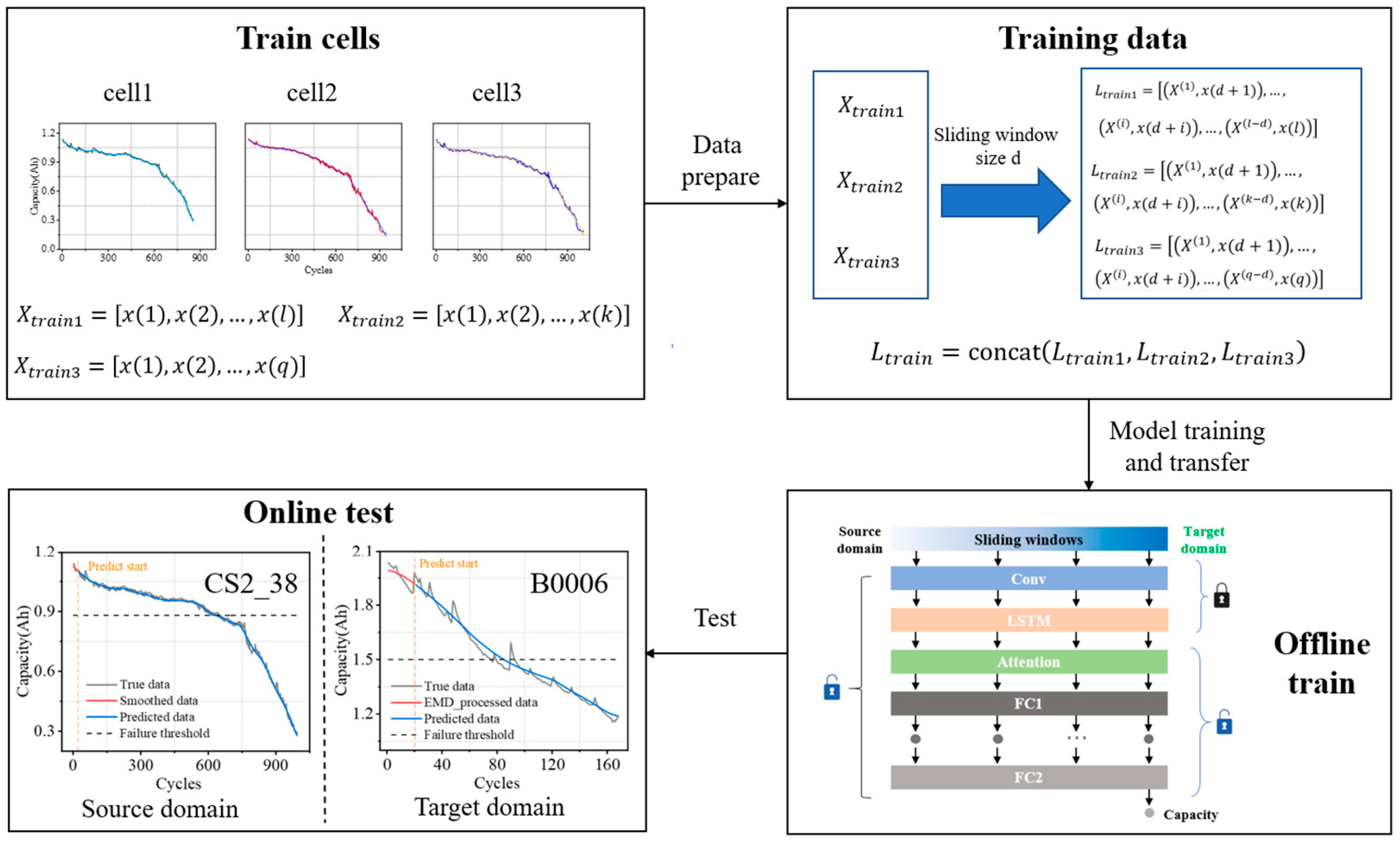
In this paper, a fast and transferable data-driven method is proposed for the prediction of battery aging trajectories under different operating conditions, and the general flow is shown in Figure 1.

2.1. Data Acquisition

In this paper, we use three different datasets CACLE, NASA, and NCM from the University of Maryland, NASA, and our laboratory [35,36].

The CALCE datasets were gathered at a stable temperature of 1 °C. During the charging phase, the battery was handled in constant current (CC) mode until its voltage reached 4.2 V, after which the mode was switched to constant voltage (CV). For the discharging phase, the battery operated in CC mode until it reached its discharge capacity, lowering the voltage to below 2.7 V. Detailed information on the CALCE datasets is provided in

Table 1. Detailed information about CALCE datasets.

Cell Number	Rated Capacity (Ah)	Voltage Range(V)	Discharge Current(A)	Temperature (°C)
CS2_35	1.1	2.7–4.2	1.1	1
CS2_36	1.1	2.5–4.2	1.1	1
CS2_37	1.1	2.2–4.2	1.1	1
CS2_38	1.1	2.5–4.2	1.1	1

, and Figure 2a illustrates the capacity variation curves of the CALCE datasets with increasing cycles.

The NASA datasets comprise aging data for four distinct types of lithium-ion batteries, obtained under three operational conditions: charging, discharging, and impedance measurements. The tests for battery charging and discharging were conducted at a constant temperature of 24 °C. During the charging phase, the battery was initially charged in constant current (CC) mode at 1.5 A until the voltage reached 4.2 V, at which point it transitioned to constant voltage (CV) mode. In the discharging process, the battery was discharged in CC mode until it hit a predetermined voltage. Figure 2b shows the capacity variation curves of NASA batteries as the number of cycles increases.

Table 2. Detailed information about NASA datasets.

Cell Number	Rated Capacity (Ah)	Voltage Range (V)	Discharge Current (A)	Temperature (°C)
B0005	2	2.7–4.2	2	24
B0006	2	2.5–4.2	2	24
B0007	2	2.2–4.2	2	24
B0018	2	2.5–4.2	2	24

presents detailed information about the NASA battery datasets.

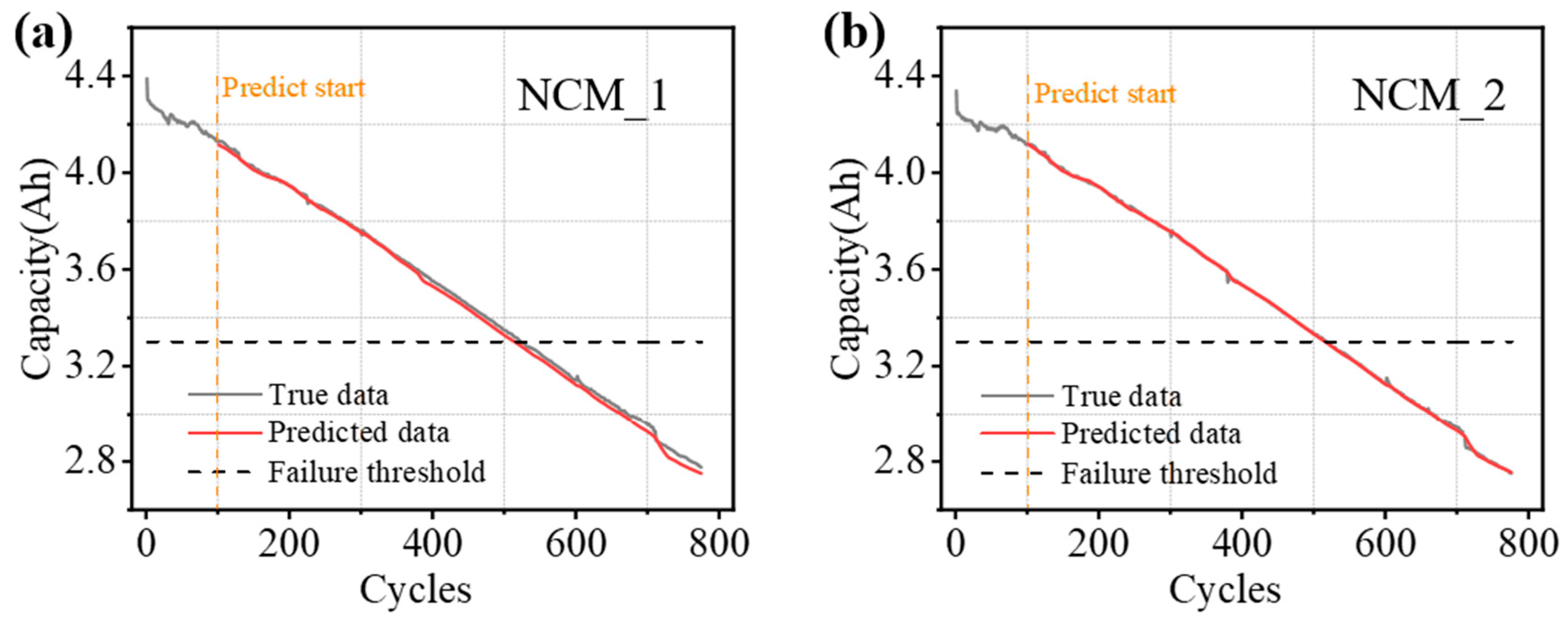
The NCM batteries from our laboratory are designed for use in deep-space environments. We have tested a total of two batteries.

Table 3. Detailed information about NCM datasets.

Cell Number	Rated Capacity (Ah)	Voltage Range (V)	Discharge Rate (C)	Temperature (°C)
NCM_1	4.4	2.5–4.3	0.2	25
NCM_2	4.4	2.5–4.3	0.2	25

provides detailed information on these NCM batteries, and the capacity change curve relative to the number of cycles is shown in Figure 2c.

2.2. Data Processing

2.2.1. Source Domain Data Processing

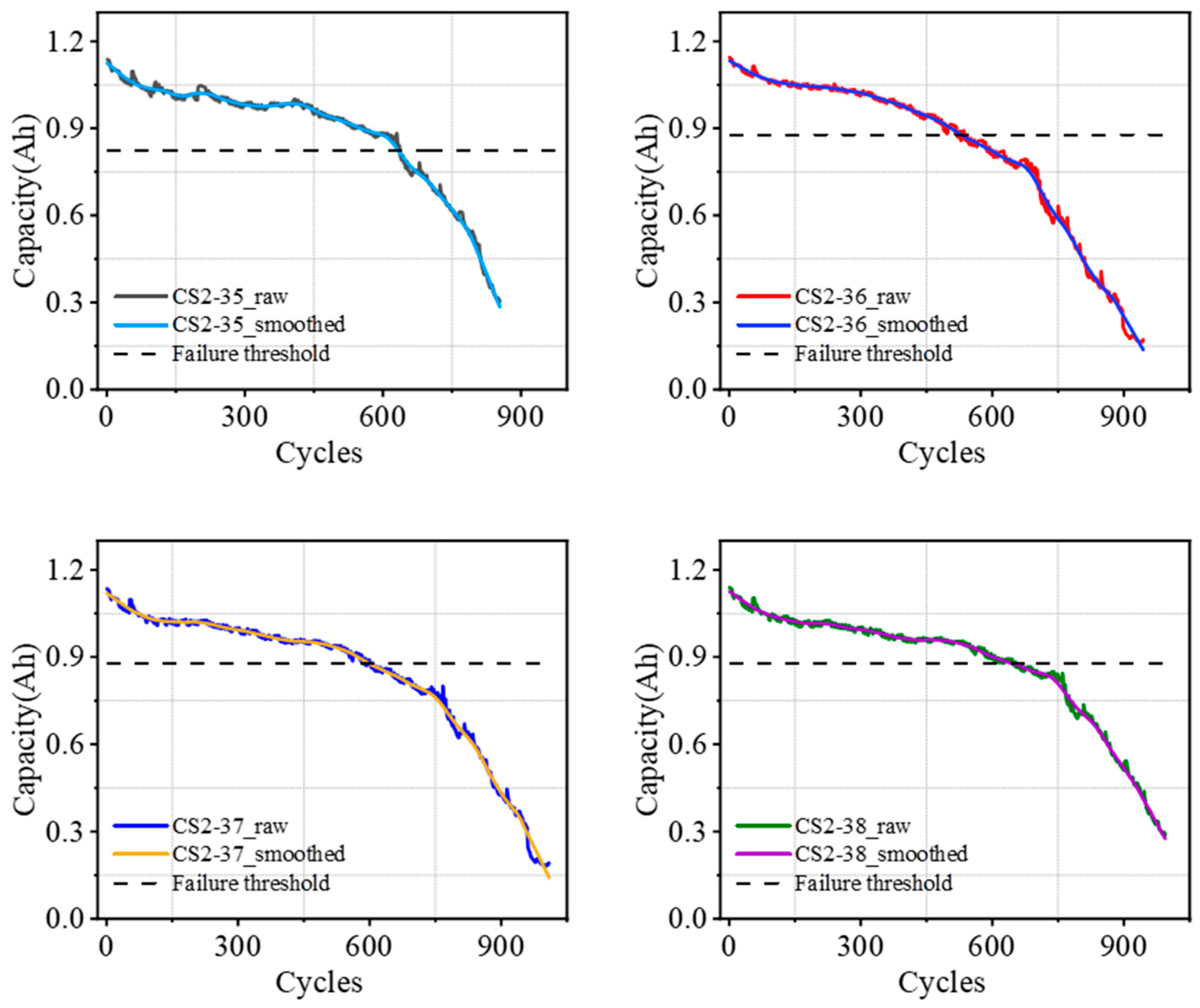
First, the source–domain CALCE battery capacity degradation data are smoothed using the Lowess method to remove some noise present in the original data and obtain a smoother trend line, which helps to better reveal the real trend of battery capacity decline rather than short-term fluctuation [37,38]. The smoothed decline curve is shown in Figure 3. Pearson correlation analysis was used to assess the correlation between the smoothed curves and the original series and the correlation coefficients are given in

Table 4. Pearson correlation coefficients between smoothed and real data for the CALCE datasets.

CS2_35	CS2_36	CS2_37	CS2_38
0.9817	0.9866	0.978	0.9778

. The results of the correlation analysis show that the Pearson correlation coefficients for each residual exceed 0.97.

2.2.2. Target Domain Data Processing

NASA batteries in the target domain exhibit an obvious capacity regeneration phenomenon. To eliminate the effect of capacity regeneration, it is essential to preprocess the raw capacity data, which is crucial for improving network training efficiency. The Lowess (Locally Weighted Scatterplot Smoothing) method, which uses source domain data, is ineffective in this context. Therefore, we utilize the CEEMDAN (Complete Ensemble Empirical Mode Decomposition with Adaptive Noise) algorithm to achieve this goal. The CEEMDAN algorithm is capable of efficiently removing noise and mitigating the inherent complexity and volatility of the raw capacity data, thus isolating the main trends of battery capacity degradation. Using the B0005 battery as an illustration, Figure 4a,b shows the RES and IMF curves of the B0005 battery capacity signal obtained through the CEEMDAN algorithm, respectively. The RES component obtained via CEEMDAN processing can fully depict the declining trend of the initial data, exhibiting a more refined pattern than the raw data. This signal-processing method facilitates a more precise examination of battery capacity degradation.

2.2.3. Training Data

After obtaining the smoothed data, the training data are obtained by means of a sliding window. Once the window size d is determined, for a training sample $\left(X^{\left(i\right)},x\left(d+i\right)\right)$ for $i=\mathrm{1,2},\dots ,l-d$ of Train cell $X_{train}$ of length $l$, the input data $X^{\left(i\right)}$ can be constructed by Equation (4) and $x\left(d+i\right)$ is the label of the input to the data.

$$X_{train}=[x\left(1\right),x\left(2\right),\dots ,x\left(l\right)]$$

(3)

$$L_{train}=\left[\left(X^{\left(1\right)},x(d+1)\right),\left(X^{\left(i\right)},x(d+i)\right),\dots ,\left(X^{\left(l-d\right)},x\left(l\right)\right)\right]$$

(4)

2.3. Aging Trajectory Prediction Framework

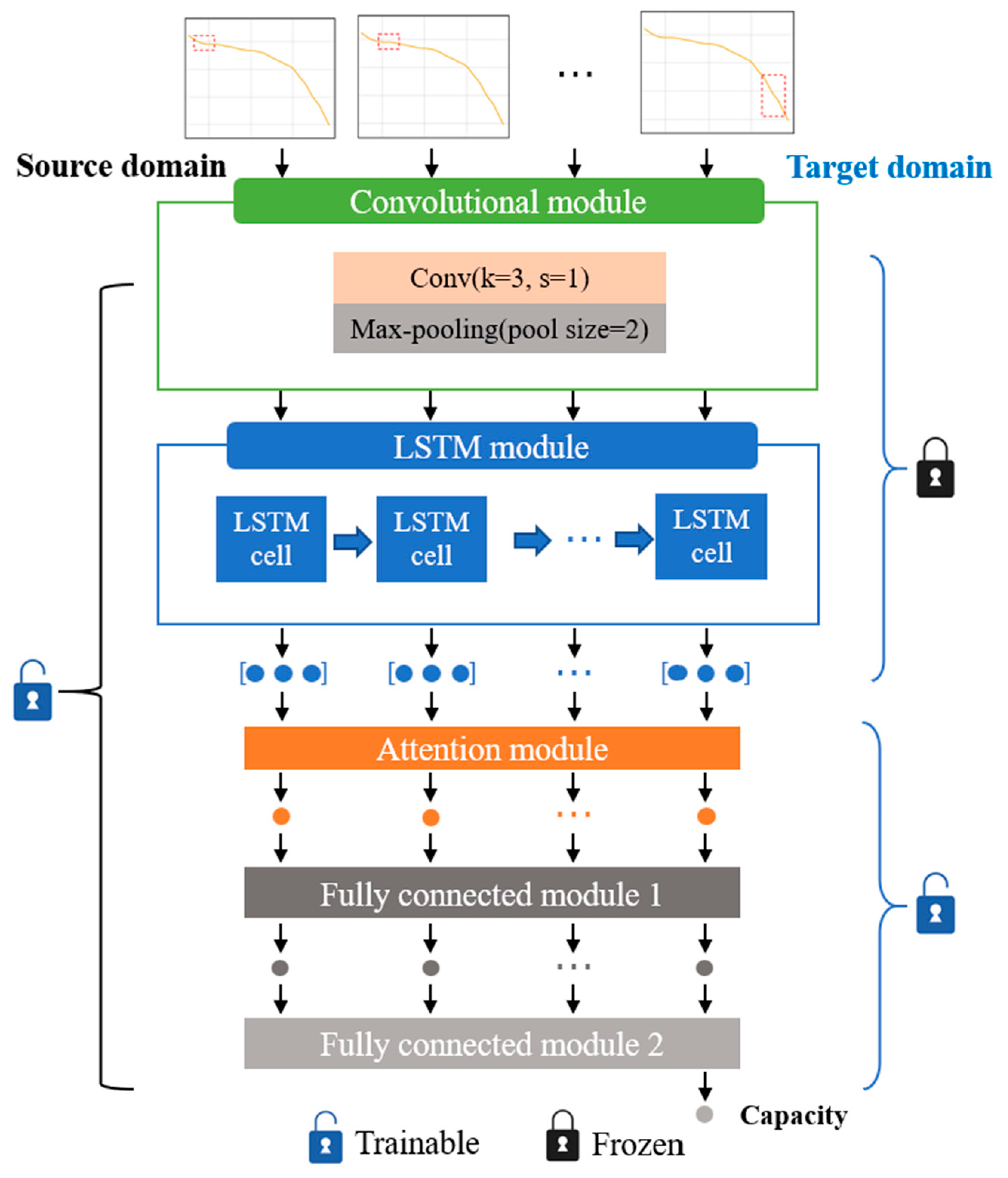
We developed a CNN-LSTM-Attention network model that integrates CNN, LSTM, and Attention mechanisms. This model extracts local features through the convolutional layer, captures sequence dependencies via the LSTM layer, and enhances the representation of key information using the Attention layer. Finally, the model outputs prediction results through fully connected layers. By combining the strengths of convolutional and sequence models and improving the ability to capture global information through the Attention mechanism, this network enhances overall model performance. The network framework is illustrated in Figure 5, showing that the input data sequentially pass through one CNN layer, one LSTM layer, one customized Attention layer, and two fully connected layers.

2.3.1. Convolutional Neural Network

The input data are first passed through a one-dimensional convolutional layer with the convolutional kernel moving along the time axis, using the ReLU activation function to increase the nonlinear capability of the network and allow the model to learn complex time series patterns, implemented by Equation (5) [39,40]. The results obtained are then subjected to a one-dimensional maximum pooling operation, implemented by Equation (6), which allows the model to extract important features from the output of the convolutional layer and reduce the number of model parameters, thus reducing the risk of overfitting and improving computational efficiency [39].

$$y^l=Relu\left(b^l+\sum _{n=1}^m{W}_n^l\ast x^{l-1}\right)$$

(5)

$$q^l=Maxpool\left(y^l\right)$$

(6)

where $x^{l-1}$ refers to the input vector of the convolutional layer $l-1$, which additionally functions as the input layer of the model, i.e., when $l$ equals 1, $x$ denotes the initial input capacity sequence, $b^l$ denotes the bias parameter, $W_n^l$ is convolution kernel’ weight parameter, m denotes the number of filters, the symbol $\ast$ represents the convolution operation, and $q^l$ is a further result of pooling $y^l$.

After the CNN layer, a fully connected (FC) layer is employed to transform the data information into a format suitable for the LSTM layer’s input. This procedure creates a linkage between the CNN layer and the LSTM layer, enabling the LSTM to capture the spatial features extracted by the CNN.

2.3.2. Long- and Short-Term Memory Network

After extracting features from the convolutional layer, temporal features are extracted using the LSTM layer to learn the temporal dependence of the data. The LSTM has a control flow similar to that of an RNN, which processes the data that pass on information as they propagate forward [41]. The difference lies in the operation within the LSTM cell. The key design of LSTM is the gating mechanism and the cell state cell. The cell state retains the current LSTM’s state information and transfers it to the next time step. The gating mechanism regulates the flow of information from the cell state. The LSTM layer comprises three gates: the forget gate, the input gate, and the output gate.

(1)

The forget gate controls the flow of information through the LSTM cells, selectively retaining or discarding information to better capture and utilize long-term dependencies in time series data. The equation is expressed as

$${\mathrm{f}}_t=\sigma \left(W_{xf}{x}_t+W_{hf}{h}_{t-1}+b_f\right)$$

(7)

where ${\mathrm{f}}_{\mathrm{t}}$ is the output of the forgetting gate, $h_{t-1}$ is the output state at moment t − 1, $x_t$ is the input vector at time t (i.e., the dataspace feature q of the FC layer reshaping), $W_{xf}$, $W_{hf}$ are the weight matrices, and $b_f$ is the bias.

(2)

The input gate determines the information being updated, which can be expressed as an input gate containing two parts, the sigmoid layer and the tanh layer. The sigmoid layer acts like the forgetting gate, outputting a value $i_t$ between 0 and 1 to determine which information needs to be updated. The equation is expressed as

$${\mathrm{i}}_t=\sigma \left(W_{xi}{x}_t+W_{hi}{h}_{t-1}+b_i\right)$$

(8)

where $W_{xi}$ and $W_{hi}$ are the weight matrices and $b_i$ is the bias.

Then, a tanh layer creates a vector of the new candidate state $\widetilde{c_t}$, and the equation is expressed as

$$\widetilde{c_t}=\tanh \left(W_{xc}{x}_t+W_{hc}{h}_{t-1}+b_c\right)$$

(9)

where $W_{xc}$ and $W_{hc}$ are the weight matrices of the state candidate vectors and $b_c$ is the bias.

The output of the input gate is jointly determined by the outputs of the sigmoid and tanh layers. The equation is expressed as

$${\mathrm{c}}_t={\mathrm{f}}_t{c}_{t-1}+{\mathrm{i}}_t\widetilde{c_t}$$

(10)

where ${\mathrm{f}}_{\mathrm{t}}$ is the output value of the forgotten gate and ${\mathrm{i}}_{\mathrm{t}}$ is the output value of the input gate.

(3)

The output gate is responsible for computing the output signal $o_t$. The equation is expressed as

$$o_t=\sigma \left(W_{xo}{x}_t+W_{ho}{h}_{t-1}+b_o\right)$$

(11)

where $W_{xo}$ and $W_{ho}$ are the weight matrices of the output gate and $b_o$ is the bias of the output gate.

${\mathrm{c}}_{\mathrm{t}}$ passes through a tanh layer and is multiplied with $o_t$ to obtain the output signal $h_t$, i.e., the combination of the output gate $o_t$ passes the information of the internal state to the external state $h_t$, as shown in Equation (12). $h_t$ is also passed to the attention layer as the input signal for the next moment.

$$h_t=o_t\tanh \left(c_t\right)$$

(12)

2.3.3. Attention Layer

Incorporating an attention layer into the model enables it to prioritize important elements within the input sequence. This enhancement simplifies the learning process and boosts the model’s overall performance. Only the outputs from preceding layers that are vital for the next stages of the model are chosen. This mechanism allows the network to concentrate selectively on specific pieces of information. Incorporating attention mechanisms into different RNN architectures has improved performance in many tasks, establishing it as an essential component of contemporary RNN frameworks. Models utilizing the attention mechanism have demonstrated strong results when applied to time series data [42,43]. To ensure training speed, we simplify the attention module as follows:

(1)

For each time step j, compute the attention score $e_{ij}$

$$e_{ij}=\mathrm{t}\mathrm{a}\mathrm{n}\mathrm{h}\left(h_j·W+b\right)$$

(13)

where $h_j$ is the LSTM output at the time step j, W is the weight, and b denotes the bias.

(2)

Normalize the attention scores by softmax function to obtain the attention weights

$${\alpha }_{ij}={\displaystyle \frac{\mathrm{e}\mathrm{x}\mathrm{p}\left(e_{ij}\right)}{\sum _{k=1}^n\mathrm{e}\mathrm{x}\mathrm{p}\left(e_{ik}\right)}}$$

(14)

where n is the number of time steps.

(3)

The output generated by the LSTM is combined with the attention weights through a weighted sum to produce the result of the attention layer, as described by Equation (15). Subsequently, the fully connected layer is used to derive the ultimate output of the CNN-LSTM-Attention model.

$$Z_i=\sum _{j=1}^n{\alpha }_{ij}{h}_j$$

(15)

2.4. Model Optimization

In the training process of deep neural networks, choosing appropriate hyperparameters (e.g., learning rate, batch size, etc.) is crucial for the accuracy and training efficiency of the model. We decided to use the Gray Wolf Optimization (GWO) algorithm mainly because of its simplicity and powerful global search capability. The GWO algorithm simulates the hunting behavior of gray wolves, and it can be optimized efficiently with a small number of parameter settings. In addition, the GWO algorithm performs well in optimization problems with large search space and complex functions and can effectively avoid falling into local optima. In contrast, Bayesian optimization, despite its advantages in dealing with high-cost objective functions, is not as good as the GWO algorithm in high-dimensional problems because of its complicated agent model construction and high computational complexity, while other optimization algorithms, such as Particle Swarm Optimization (PSO) and Genetic Algorithms (GA), also have certain global search capabilities but often require more parameter adjustments and are prone to fall into local optimization in some cases. Therefore, considering the characteristics of the problem and the optimization requirements, we believe that GWO algorithm is the best choice at present. Specifically, when using the GWO algorithm for hyperparameter optimization, a set of gray wolf groups is first initialized, where each gray wolf represents a set of hyperparameters. Then, the positions of the gray wolves are iteratively updated, and the optimal hyperparameter combination is gradually approximated by evaluating the strengths and weaknesses of each gray wolf based on the fitness function. Eventually, after many iterations of optimization, the gray wolf population converges to an optimal or near-optimal hyperparameter configuration, which significantly improves the performance of the deep neural network. Compared with other optimization algorithms, the optimization process of the gray wolf algorithm is faster. Here, we optimize four hyperparameters, namely, the number of filters in the convolutional layer, the initial learning rate, the L2 regularization coefficient, and the batch size, to determine the hyperparameters to be used for the final model training.

2.5. Specific Layer-Based Transfer Learning

A deep transfer learning strategy is designed to enable real-time personalized predictions of battery aging trajectories by utilizing insights from diverse yet related battery degradation data. Initially, the transfer learning model undergoes retraining with preliminary capacity degradation data from batteries within the target domain and then the retrained model is used to predict subsequent decline trajectories of its batteries. The source domain is the initial training domain for pre-trained models, which usually has a large amount of labeled data and rich features. The target domain is the domain of the transfer learning application, which usually has less data and scarce labeled data. The data distribution, feature space, and task objectives in the source domain can be different from the target domain, but can also have some degree of similarity. Deep transfer learning models are flexible and can be quickly adapted to new operating conditions by dynamically fine-tuning specific network layers [44]. We adapt to the new battery by tuning the attention layer and fully connected layers of the network. This is shown in Figure 6.

2.6. Model Evaluation Criteria

To assess the effectiveness of the proposed approach, we employ mean absolute error (MAE), mean absolute percentage error (MAPE), and root mean square error (RMSE) as our evaluation metrics. Lower values of MAE, MAPE, and RMSE indicate the greater accuracy of the proposed method. The calculation formulas are as follows.

$$MAE={\displaystyle \frac{1}{n}}\sum _{i=1}^n\left|\widehat{y_i}-y_i\right|$$

(16)

$$MAPE={\displaystyle \frac{1}{n}}\sum _{i=1}^n\left|{\displaystyle \frac{\widehat{y_i}-y_i}{y_i}}\right|\times 100\%$$

(17)

$$RMSE=\sqrt{{\displaystyle \frac{1}{n}}\sum _{i=1}^n{\left(\widehat{y_i}-y_i\right)}^2}$$

(18)

where $y_i$ is the actual capacity data, $\widehat{y_i}$ is the predicted capacity data, and n is the number of cycles.

The predicted EOL is obtained when a battery’s capacity falls to the predetermined failure threshold. The error metric (Error Metric, EM) in Equation (19) quantifies the absolute error between the actual EOL and the predicted EOL for each cell; the accuracy metric (AM) detailed in Equation (20) is used as the relative error of the predicted EOL. Since it is not an end-to-end prediction and cannot output RUL directly, we calculate the accuracy of RUL prediction by using these two metrics.

$$EM=\left|EOL-\widehat{EOL}\right|$$

(19)

$$AM=\left\{1-{\displaystyle \frac{\left|EOL-\widehat{EOL}\right|}{EOL}}\right\}\times 100\%$$

(20)

Notably, the developed model was implemented on a computer equipped with AMD (Advanced Micro Devices, Inc., Santa Clara, CA, USA) R7-6800HS CPU, NVIDIA GeForce RTX 3060 GPU, and 16G of RAM using TensorFlow backend for Python 3.9.

3. Results Analysis

To validate the proposed framework, tests were carried out on both source and target domains to comprehensively showcase the qualitative findings. Subsequently, the future capacity and RUL prediction outcomes were analyzed in detail. The sliding window d is initially set at 20. The CALCE battery is considered to have reached its EOL once its capacity diminishes to 80% of the rated capacity. For the NASA and NCM batteries, they are considered to have achieved their EOL when their capacity falls to 75% of the initial rated capacity.

3.1. Aging Trajectory Prediction Results

In the source domain, we use the cross-validation method to divide the CALCE dataset into training and testing sets, as shown in Figure 7. In the cross-validation process, one cell is sequentially selected as the test cell and the remaining three cells are used as the training cells for a total of four iterations. In each iteration, the model is trained using the training set and the model performance is evaluated using the test cell. By validating models on multiple subsets, cross-validation provides a more stable and reliable assessment of model performance, reducing the impact of randomness associated with a single training-validation division. This process was repeated for four iterations and the test results at the test battery are shown in Figure 8. The capacity data from the 1st to the 20th cycle were used as the first input for the test, i.e., the 21st cycle was the first prediction point.

We also compared this algorithm with other methods and the final results are shown in

Table 5. Prediction results of CALCE batteries using the proposed method and the other comparative methods.

Cell Number	Model	MAE (Ah)	MAPE	RMSE (Ah)	EM	AM
CS2_35	CNN	0.0314	4.58%	0.0392	25	95.67%
	LSTM	0.0219	2.94%	0.0287	19	96.71%
	CNN-LSTM	0.0113	2.39%	0.015	15	97.4%
	CNN-GRU	0.017	3.04%	0.0183	16	97.23%
	CNN-LSTM-Attention	0.0102	1.33%	0.0133	9	98.44%
CS2_36	CNN	0.0394	4.93%	0.0472	32	93.83%
	LSTM	0.0253	3.19%	0.0305	22	95.76%
	CNN-LSTM	0.0161	2.82%	0.021	17	96.72%
	CNN-GRU	0.0218	3.17%	0.0291	18	96.53%
	CNN-LSTM-Attention	0.0103	1.98%	0.0141	15	97.11%
CS2_37	CNN	0.0417	4.15%	0.0375	34	94.19%
	LSTM	0.029	2.91%	0.0314	26	95.56%
	CNN-LSTM	0.0155	2.79%	0.0241	21	96.41%
	CNN-GRU	0.0176	3.13%	0.0263	22	96.24%
	CNN-LSTM-Attention	0.0096	1.78%	0.0131	17	97.09%
CS2_38	CNN	0.0407	4.02%	0.0449	36	94.21%
	LSTM	0.0242	2.47%	0.0276	23	96.3%
	CNN-LSTM	0.0187	2.13%	0.0231	17	97.27%
	CNN-GRU	0.0194	2.75%	0.0218	21	96.62%
	CNN-LSTM-Attention	0.0087	1.15%	0.0113	12	98.07%

. As we can see, our method achieves the lowest MAE, MAPE, RMSE, and EM and the highest AM on each cell. The results show that the algorithm predicts RUL more accurately and stably than other methods.

The model obtained from the training of CS2_35, CS2_36, and CS2_37 is finally selected as the source domain model for the subsequent transfer work. Our proposed CNN-LSTM-Attention model predicts the results on this set of experimental test cells with MAE of 0.0087 Ah, MAPE of 1.15%, RMSE of 0.0113 Ah, EM of 12, and AM of 98.07%. The hyperparameters obtained by the Gray Wolf optimization algorithm for this set of experiments are shown in

Table 6. Optimization hyperparameters used by the model.

Filter Numbers	Initial Learning Rate	L2 Regularization Coefficient	Batch Size
52	0.00082	0.01	64

.

3.2. Transfer Learning Results

In the target domain NASA batteries, batteries B0005 and B0018 are used as train batteries, the attention and fully connected layers of the model used in the source domain are fine-tuned, and the retrained model is utilized to predict the future capacity and RUL of batteries B0006 and B0007; the prediction results are shown in Figure 9. The evaluation results of the future capacity and RUL prediction of the two batteries using the migrated obtained CNN-LSTM-Attention model are given in

Table 7. Prediction results of battery B0006 and B0007.

Battery	MAE (Ah)	MAPE	RMSE (Ah)	EM	AM
B0006	0.0248	1.65%	0.0301	9	88%
B0007	0.0115	0.72%	0.0162	8	93.65%

. The evaluation results of other comparison methods for each battery prediction are given. The predicted capacity of battery B0006 was below the EOL at the 75th cycle. The capacity and RUL prediction results are depicted in Figure 9a, from which it can be seen that the transfer-obtained model predicts the capacity degradation trend well. The predicted results are 0.0248 Ah for MAE, 1.65% for MAPE, 0.0301 Ah for RMSE, and 88% for AM. Figure 9b shows the predicted results for battery B0007. At the 126th cycle, the true failure threshold was reached and the MAE, MAPE, and RMSE were calculated to be 0.0115 Ah, 0.72%, and 0.0162 Ah, respectively, with an AM of 93.65%. These results show that the fine-tuned model can accurately predict future capacity and RUL without full training.

The evaluation results of other comparative methods for the prediction of the two batteries are given in

Table 8. Prediction results of battery B0006 and B0007 using the other comparative methods.

Battery	Model	MAE (Ah)	MAPE	RMSE (Ah)	EM	AM
B0006	CNN	0.1181	5.28%	0.1224	24	68%
	LSTM	0.0619	3.87%	0.083	15	80%
	CNN-LSTM	0.0328	2.79%	0.0413	11	85.33%
	CNN-GRU	0.0412	2.9%	0.0495	12	84%
B0007	CNN	0.103	5.32%	0.1137	21	83.33%
	LSTM	0.0544	3.37%	0.0625	15	88.1%
	CNN-LSTM	0.0227	1.89%	0.0311	11	91.27%
	CNN-GRU	0.0263	2.27%	0.0289	11	91.27%

. The CNN-LSTM-Attention model obtained by transfer learning has the best prediction on both batteries, achieving the lowest MAE, MAPE, RMSE, and EM and the highest AM compared to the other methods.

In the target domain NCM batteries, NCM_1 and NCM_2 are used as retrained batteries, respectively, and the attention and fully connected layers of the model used in the fine-tuned source domain are used to predict the future capacity and RUL of the other battery using the retrained model. Since the battery capacity fluctuates a lot in the initial stage due to some external reasons at the time of testing, the 101st cycle was chosen as the starting point for prediction, and the prediction results are shown in Figure 10. The results of the evaluation of the prediction of the two cells using the model obtained by transfer learning are given in

Table 9. Prediction results of battery NCM_1 and NCM_2.

Battery	MAE (Ah)	MAPE	RMSE (Ah)	EM	AM
NCM_1	0.0162	0.5%	0.019	8	98.47%
NCM_2	0.0041	0.12%	0.0062	3	99.42%

, and the results of the evaluation of the prediction of the 2 cells by the other comparative methods are given in

Table 10. Prediction results of battery NCM_1 and NCM_2 using the other comparative methods.

Battery	Model	MAE (Ah)	MAPE	RMSE (Ah)	EM	AM
NCM_1	CNN	0.047	5.52%	0.0522	29	94.44%
	LSTM	0.0319	2.11%	0.0375	18	96.55%
	CNN-LSTM	0.0223	1.54%	0.027	12	97.70%
	CNN-GRU	0.0289	1.87%	0.0302	14	97.32%
NCM_2	CNN	0.0215	3.18%	0.0248	21	95.95%
	LSTM	0.011	1.92%	0.0153	12	97.69%
	CNN-LSTM	0.0092	1.74%	0.012	8	98.46%
	CNN-GRU	0.0103	1.95%	0.0147	10	98.07%

. It can be seen that the values of MAE, MAPE, RMSE, and EM are lower than those of the other four algorithms, and the value of AM is higher than the other four algorithms, for the finely-tuned CNN-LSTM-Attention model, on both NCM_1 and NCM_2 cell.

3.3. Validation of the Effectiveness of Transfer Strategy

To demonstrate the effectiveness of the present transfer strategy, we have conducted two sets of comparison experiments. First, in the first set of experiments, only the last two fully connected layers of the source domain network model were fine-tuned, which is the usual way of most current studies. After retraining is completed, the test cell in the target domain is tested, and several important metrics are given in

Table 11. Prediction results of fine-tuning only the fully-connected layers.

Battery	MAPE	RMSE (Ah)	AM
B0006	1.96%	0.0396	86.67%
B0007	0.81%	0.0181	90.48%
NCM_1	0.76%	0.0252	97.70%
NCM_2	0.17%	0.0113	98.46%

. By comparison with Table 7 and Table 9, it can be seen that the transfer strategy used in this paper has a more significant performance improvement compared with fine-tuning only the fully connected layers. In the second set of experiments, we fine-tuned the source domain network model in its entirety and analyzed the prediction effect on test batteries in the target domain, and the prediction results are shown in

Table 12. Prediction results of fine-tuning the entire deep network.

Battery	MAPE	RMSE (Ah)	AM
B0006	1.42%	0.0255	89.33%
B0007	0.65%	0.0149	95.24%
NCM_1	0.33%	0.0167	98.85%
NCM_2	0.10%	0.0046	99.42%

. It can be seen that the prediction effect has a slight improvement compared to the proposed transfer strategy. However, the time cost spent on training is significantly higher, and there is a risk of overfitting the complete deep network fine-tuned with a small number of data samples.

4. Conclusions

This work develops a CNN-LSTM-Attention-based approach combined with transfer learning for battery future capacity estimation and RUL prediction under different operating conditions. In the source domain, the model training samples the Gray Wolf optimization algorithm to optimize the hyperparameters of the model. In the model transfer phase, the impact of capacity regeneration on model prediction is first mitigated using the CEEMDAN algorithm for NASA batteries with an obvious capacity regeneration phenomenon. The CNN and LSTM layers of the source–domain model are frozen during retraining, and the attention and fully connected layers are fine-tuned for the NASA and self-tested NCM batteries. The results show that the proposed network model effectively improves the accuracy and stability of the battery’s future capacity estimation. In addition, the application of transfer learning solves the training problem in the data-scarce domain and demonstrates the model generalization capability in new application scenarios.

In the following work, we plan to improve the proposed RUL prediction method for lithium-ion batteries by incorporating uncertainty assessment, which will provide valuable indicators for the reliability of the prediction results while ensuring prediction accuracy.