1. Introduction
Problems with input and output sequences of various lengths are common in many applications. These tasks are usually referred as sequence-to-sequence (Seq2Seq) [
1] prediction and find natural applications in natural language processing [
2], for tasks such as translation, question answering, text generation, etc. Many of these applications can be traced back to the problem of the next token prediction, which is a classification task [
3]. In regression settings, predictions with input and output sequences of different lengths are rarer. In these situations, sliding-window approaches are more common, in which an algorithm is trained by taking a fixed number
n of past time steps to predict a fixed number
m of future steps [
4]. However, in some applications, working with variable length sequences can be advantageous, or even mandatory, both to keep all the information available up to a certain moment and to predict sequences with a variable number of future steps, possibly unknown a priori. Examples are situations in which the algorithms must predict all future steps until their value reaches a certain threshold, and the number of steps above the threshold is itself a quantity of interest.
Managing input and output sequences with different numbers of elements represents a challenge, because common deep learning libraries are designed to work with models with input and output sequences of constant lengths [
5]. While the different length input problem can be easily solved through padding and the introduction of a masking layer, the different length output problem presents complications that still make it a subject of research. In this paper, we present two methodologies for dealing with the problem of variable and unknown length predictions [
6]. The first, more commonly used, consists of predicting one step at a time, until a certain stop condition is met. The second, to our knowledge never described in the literature, predicts a multivariate output of constant length in a single step, of which only a subset of the components represent meaningful values, while the others are equivalent to padded values, which must be eliminated through a post-processing procedure.
We applied and compared these two methodologies in simultaneous State of Health (SoH) trajectory prediction and Remaining Useful Life (RUL) estimation in lithium-ion batteries. These estimates are essential for Battery Management Systems (BMSs), electronic systems responsible for several tasks such as protection [
7], cell balancing [
8], thermal management [
9], state estimation [
10,
11], and diagnosis and prognosis [
12]. Accurate predictions of the SoH trajectory and estimations of the RUL are crucial as they are directly linked to the overall performance of the battery [
13]. Additionally, these quantities are essential to determine when the battery has reached its second-life [
14] and when it should be recycled [
15]. SoH is defined as the ratio of the battery’s current maximum capacity to its nominal capacity [
16]:
RUL is defined as the number of remaining cycles above a critical SoH threshold, required for optimal and safety operation. For electric vehicles, this SoH threshold is typically set between 70% and 80%, as performance and reliability tend to degrade rapidly below these values. In contrast, for energy storage systems where there is less battery stress, the threshold is generally set between 30% and 40% [
14]. In this study, we consider the RUL threshold to be 70%.
We have designed and evaluated algorithms to predict, at each battery cycle, all future SoH values until the end of the first life (SoH trajectory), based on the SoH values of past cycles (history data). The RUL is then obtained directly from the length of the predictions. To our knowledge, this is the first method of joint estimation of the future SoH trajectory and the RUL in which the consistency between these two predictions is guaranteed.
2. Materials and Methods
The discussed methods are designed to deal with numerical sequences of different lengths and are based on recurrent neural networks. At each step, the goal is to predict the entire future sequence (of unknown length), given all the past steps. We work under the assumption that, although unknown a priori, the end of a sequence can be uniquely determined, for example, when the sequence reaches a value above or below a certain threshold.
All the models described have been implemented in python using keras library.
2.1. Autoregressive One-Step-at-Time Prediction Model
2.1.1. Autoregressive Model Description and Architecture
The Autoregressive one-step-at-time prediction model mirrors a Seq2Seq architecture. The general scheme of a Seq2Seq architecture includes two main elements: an encoder and a decoder. The encoder has the task of taking the input sequence and processing it, one component at a time, until it creates an internal state that efficiently encodes the entire input. Then, the encoded state is passed to the decoder, which has the task of generating the output sequence. The decoder operates by predicting one step at a time and taking the output generated as input for the next prediction in an autoregressive way, until a stopping condition is met. This stopping condition can be exceeding a certain number of steps, the emission of the <eos> (end of sequence) character in the case of textual tasks, or, in the application analyzed in this paper, the emission of a value above or below a certain threshold.
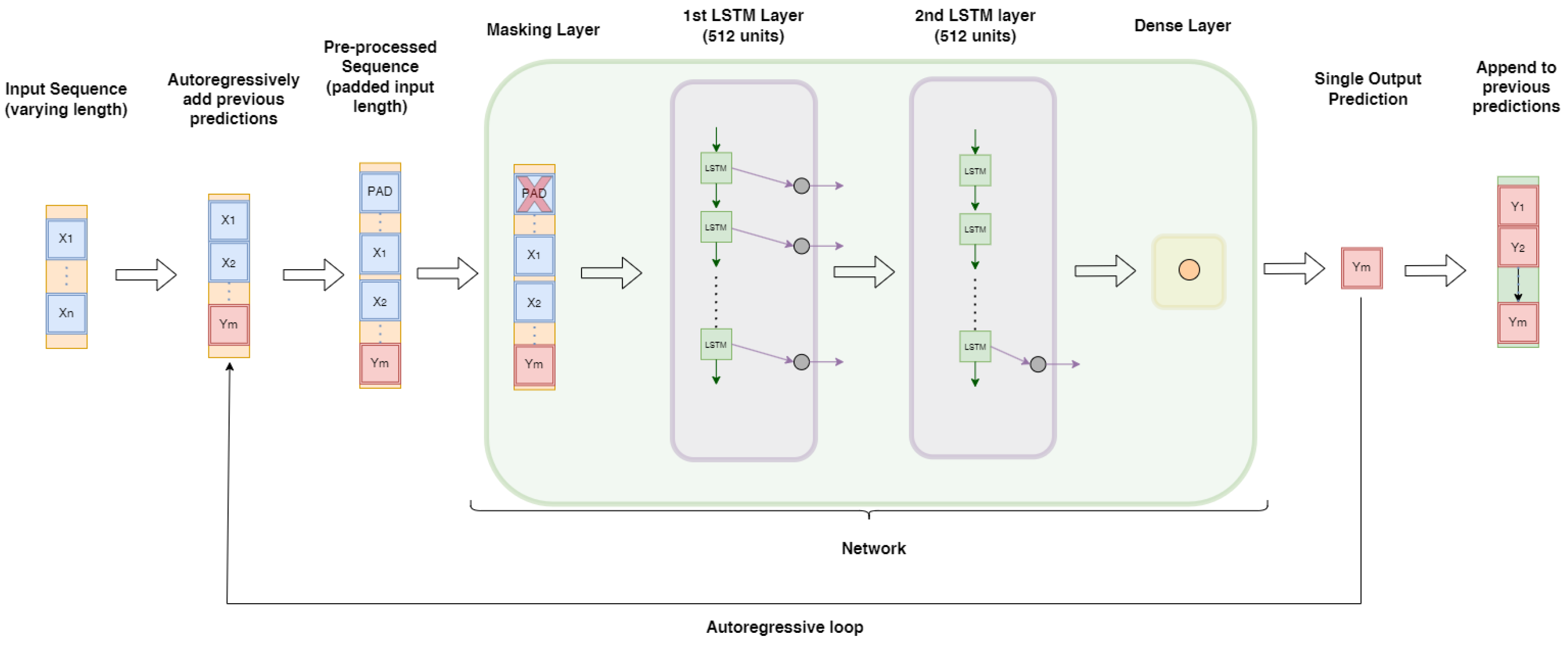
Figure 1 summarizes the Seq2Seq architecture.
In this study, we opted for a simplified version of the Seq2Seq model, in which the encoder and decoder functions are performed by the same architecture. In particular, the network is composed of the following:
A masking layer, to ignore the input padding values.
Two stacked Long Short-Term Memory (LSTM) layers of 512 neurons each.
A final dense layer with a linear activation function and an output size of 1.
Initially, all the input is processed one step at a time, without any input being created (warm-up phase). Subsequently, the same network begins the output generation, proceeding autoregressively. The procedure is shown in
Figure 2.
2.1.2. Data Preparation for Autoregressive Model
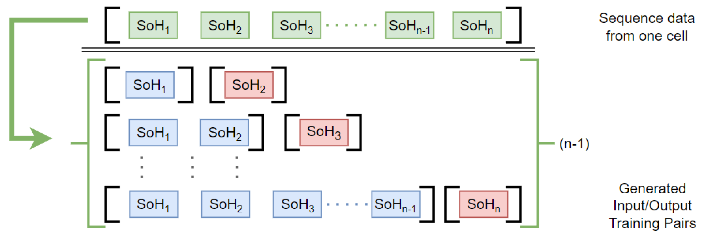
Data relating to cycles with SoH lower than the chosen threshold are removed from the dataset, with the exclusion of the first step below the threshold, which is maintained. Data are then normalized to the 0–1 range. Subsequently, from a sequence of
n steps,
input and output pairs are created. The input sequences have progressively greater length as the number of past steps grows, while the output always has dimension 1 and is constituted by the observation immediately following the last step of the input. This procedure is summarized in
Figure 3.
Since deep learning libraries require the input to be of constant length, the maximum length among training input sequences is calculated, and all sequences of shorter length are pre-padded with the arbitrary value −1. This plays the role of the masking value, and steps with this number are ignored and skipped by the masking layer. Pre- and post-padding procedures are represented in
Figure 4.
2.1.3. Autoregressive Model Implementation
The model is trained using only real sequences as input (teacher forcing). In this way, the training is more stable and faster. Predictions generated by the model are fed autoregressively into the model itself only in the test and deployment phases.
Making the model work autoregressively during training, although possible, would require a complicated low-level implementation of custom loops. Furthermore, the training would require a much larger number of operations, which, due to their intrinsic sequentiality, could not benefit from GPU parallelization. As a consequence, training would be extremely slow even with an average/small number of samples.
2.2. One-Time Multi-Step Prediction Model
2.2.1. OTMS Model Description and Architecture
In the OTMS model, to our knowledge never described before, the input is processed one step at time in a similar way to the previous model, while the output is created with a single multi-step prediction. The network is composed of the following:
A masking layer, to ignore the input padding values.
Two stacked LSTM layers of 512 neurons each.
A final dense layer with linear activation function and output size n.
The dimension
n of the last layer is chosen to be large enough to contain all the steps of any prediction. In the generated outputs, only a subset of steps have meaningful values, while the others are to be considered as padded values and must be removed through a post-processing procedure. The identification of the cutting point does not cause problems because, according to the hypotheses, it can be univocally determined. We remind that, in the applications studied in this work, the cutting point is the first prediction that falls below the chosen threshold (0.7 SoH). The OTMS model functioning is summarized in
Figure 5.
2.2.2. Data Preparation for OTMS Model
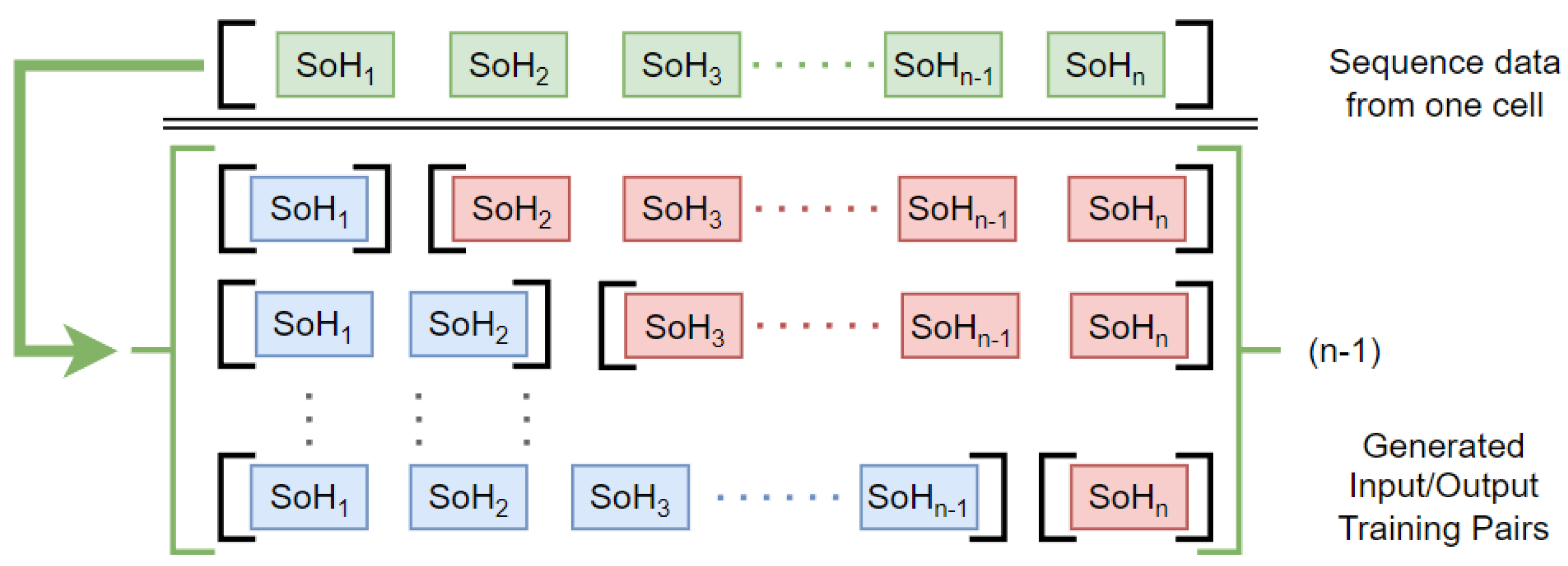
Data relating to cycles with SoH lower than the chosen threshold are removed from the dataset, with the exclusion of the first step below the threshold, which is maintained. Data are then normalized to 0–1 range. Subsequently, for each cell and for each cycle number
k of the cell, an input/output pair is created, with the input sequence consisting of measured SoH values for the first
k cycles, and the target sequence consisting of SoH values from the cycle
until the first cycle where SoH is under the threshold. This procedure is summarized in
Figure 6.
In order to have all the inputs (outputs) of the same length, pre-padding (post-padding) with the value −1 is then applied, as shown in
Figure 4.
2.2.3. OTMS Model Implementation
We have designed a custom loss function, reported in Equation (
2), that calculates the error only on predicted steps corresponding to steps not padded in the true sequences, masking the other steps.
is the indicator function,
is the
k-th component of the prediction for sequence
i made at cycle
j, len(i) is the true length of the sequence
i,
is the length of the padded sequences, and
N is the total number of sequences in the training set.
It is essential that, during training, the masking is based only on the true sequences, and that is why the indicator function in the custom loss depends only on
. Masking based on the generated output would introduce non-differentiable operations in the loss function, with consequent interruption of the computational graph for the calculation of the gradient via automatic differentiation [
17] and the impossibility of training the network correctly via gradient descent.
2.3. Dataset
Due to the time-consuming nature of extracting battery degradation data, only a limited number of battery datasets are publicly available. Most researchers in this field rely on online battery datasets, such as those provided by NASA [
18] and CALCE [
19]. In this paper, we analyze a newly available online battery dataset [
20]. This dataset includes voltage, current, and temperature measurements from six LG 2.5 Ah 18650 NMC batteries, recorded under various conditions. The discharging profiles followed the UDDS, US06, and LA92 driving cycle protocols, along with six random combinations of these cycles (referred to as Mixed 1 through Mixed 6). For recharging, constant-current constant-voltage profiles were utilized. After initial cycles at different temperatures, the batteries were aged at a consistent temperature of 35 °C.
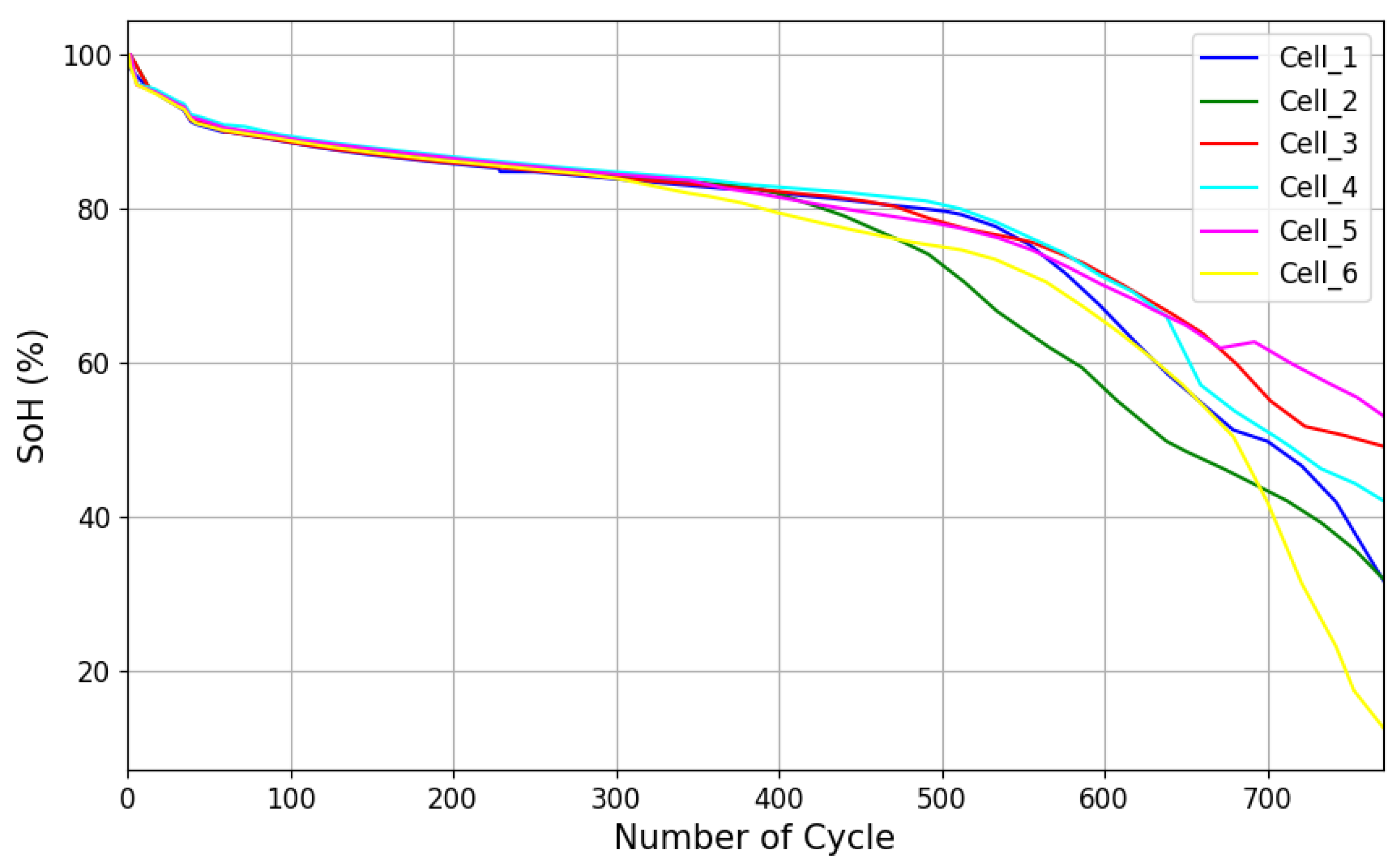
Figure 7 shows the SoH trajectories of the NMC cells. We can notice that, at the beginning, all the battery cells have similar SoH patterns. As we proceed further into the degradation stage, especially after the “knee-point”, the cells’ behavior becomes more unpredictable. This phenomenon is based on complicated electrochemical internal reactions, which lead to capacity and power fade, due to several cell losses such as lithium inventory, active material, and conductivity [
21]. A summary of the main features of the recorded data is reported in
Table 1.
2.4. Training and Evaluation
We used a cross-validation-like approach to evaluate and compare the algorithms’ performance. Specifically, we trained 6 OTMS models and 6 Autoregressive models on 6 different datasets. Each dataset was obtained by reserving the data from one cell as a test set and keeping the data from the other 5 cells for training and validation, with the proportions 80% for training and 20% for validation. The training of every model was performed using the loss function mean squared error (MSE), Adam optimizer with a 0.001 learning rate, a batch size of 32, and an early stopping mechanism with patience 5 on validation error. No optimization was made on these parameters, as it was outside the scope of this analysis.
After the training, models’ performances were evaluated by comparing the predictions on the test sets with the true data. The estimated numbers of remaining useful cycles, equal to the numbers of cycles before reaching 70% SoH in predicted sequences, were compared with the same numbers calculated on the observed sequences using the absolute error. The RUL test error for the prediction at cycle
j for the sequence
i is therefore
The errors from Equation (
3) are then averaged on the 6 models and plotted.
To compare errors in SoH trajectories, the pairs of predicted/true SoH sequences were cut as soon one of the two reached 70% SoH, and the Root Mean Squared Error (RMSE) and Mean Absolute Error (MAE) were calculated on these cut sequences.
The errors from Equations (
4) and (
5) are then averaged across the cells and plotted.
Finally, we also considered the “overall” error, obtained as the mean of the average errors at every cycle.
3. Results
In
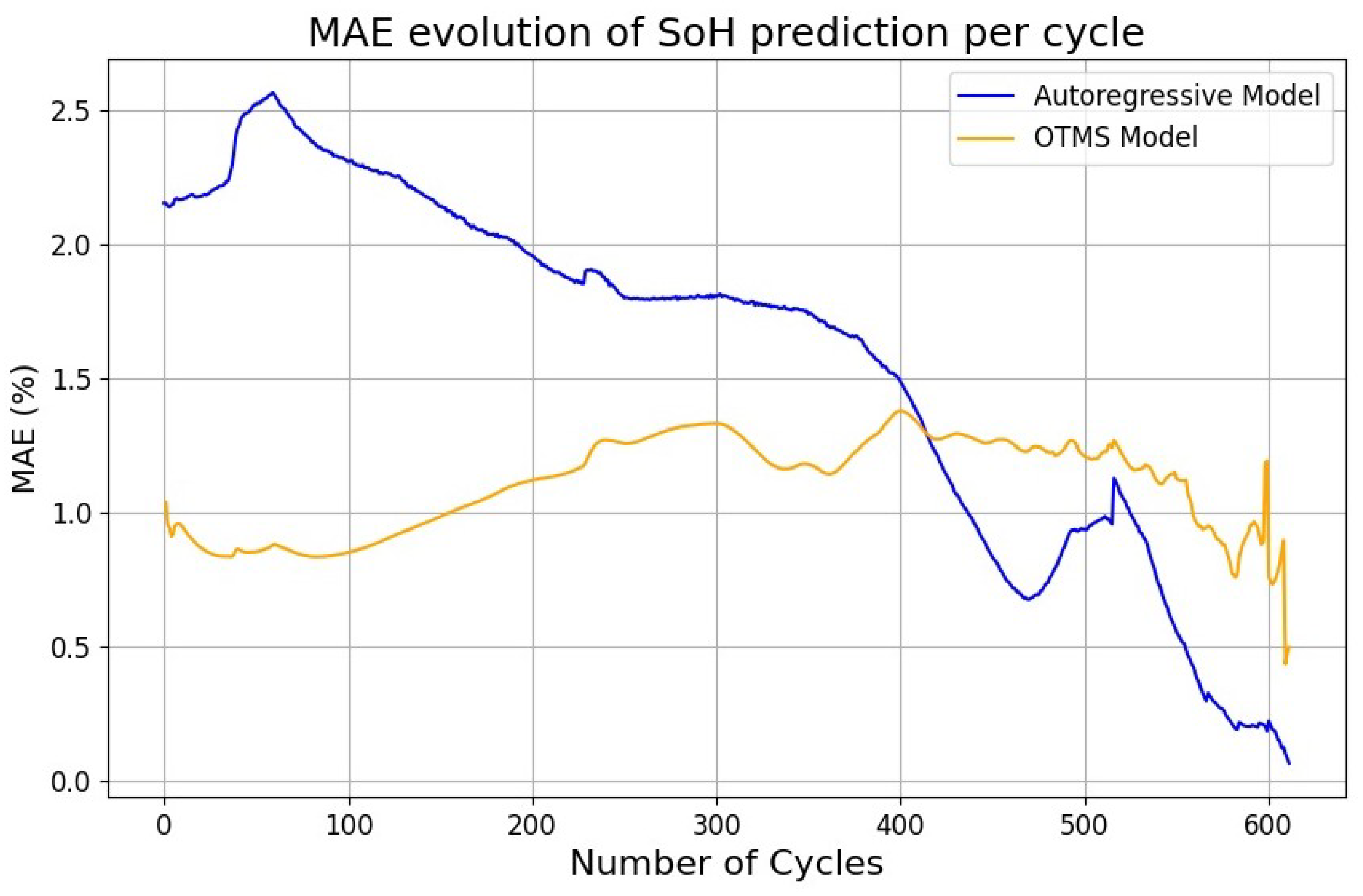
Figure 8, average models’ performances for SoH prediction throughout various degradation stages are represented. In the early stage, the Autoregressive model achieves an MAE around 2.5%, but as we move further into the degradation stage, the performance improves, reaching a final MAE around 0.25%. Conversely, the error of the OTMS model is approximately stable between 1% and 1.5% throughout all the cycles, except the very last cycles before 70% SoH. The overall SoH prediction MAE of the Autoregressive model is 1.57%, while for the OTMS model is 1.10%.
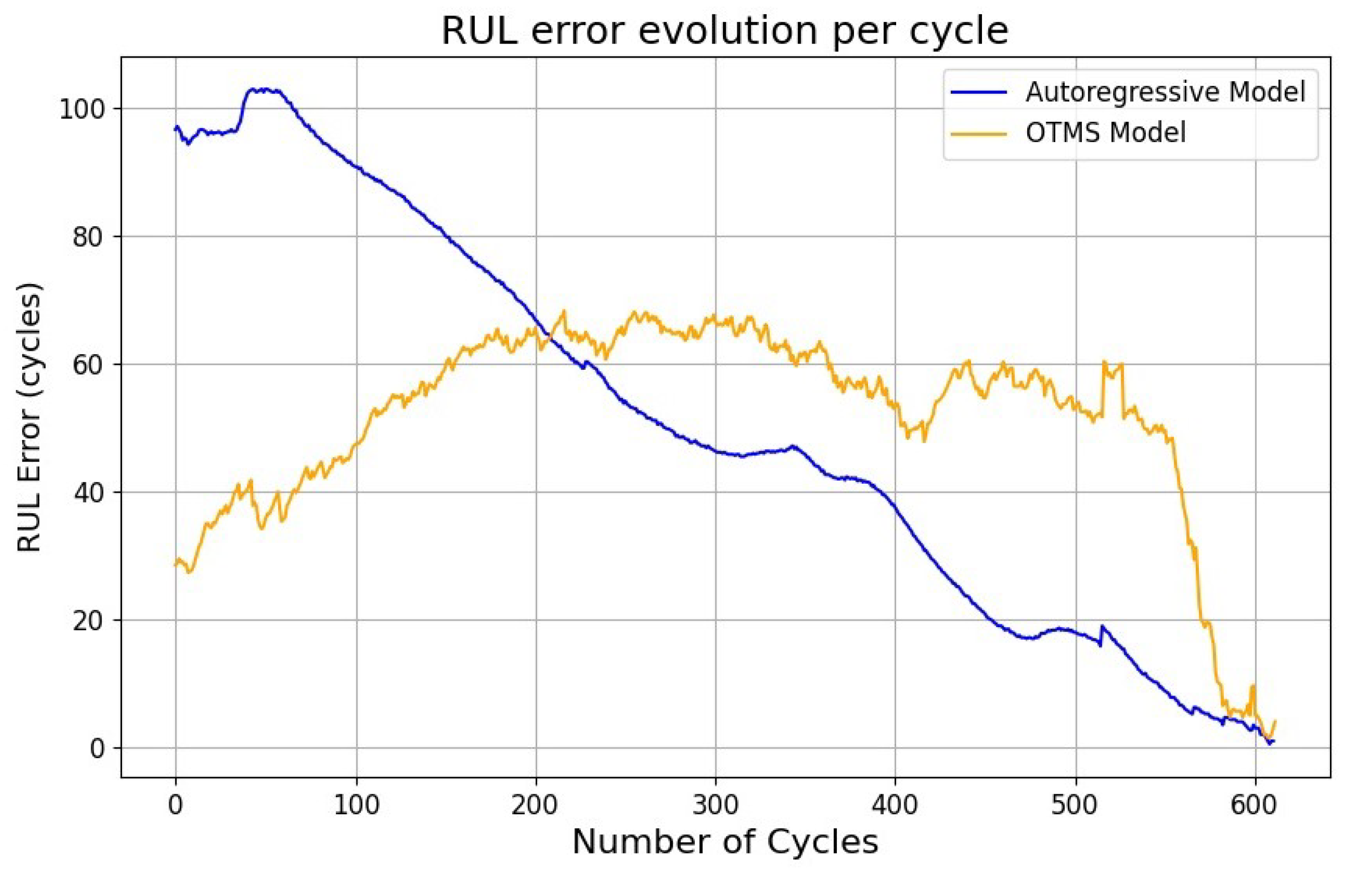
Figure 9 reports the RUL estimation error evolution for every cycle until 70% SoH. The errors of the Autoregressive model are high in the early stages, but then they steadily decline towards zero. Conversely, the OTMS model achieves low errors in the early cycles, then they increase, stabilizing around an average error of 60 cycles, and finally they fall towards 0 at the very end of the useful life. The overall RUL error of the Autoregressive model is 50.7 cycles, while for the OTMS model, it is 51.6 cycles.
In
Table 2 the SoH and RUL errors for specific degradation stages (50, 150, 300, 450) are reported, while
Figure 10 shows the SoH trajectory predictions for one test cell at the same stages.
4. Discussion
The presented models show similar overall errors both in SoH trajectory predictions and RUL estimations. Errors of the Autoregressive model are higher in the first cycles both for the RUL and the SoH trajectory, and then they decrease with the cycles as the available information increases and the future steps to be predicted are reduced. This behavior is consistent with what one might expect: for the first cycles, predictions are made based on little information, and moreover, a greater number of steps for each predicted sequence are required before reaching 70% SoH. During these steps, the autoregressive nature of the model inevitably leads to an accumulation of errors. This accumulation is exacerbated by the fact that the Autoregressive model was trained using teacher forcing, meaning that during training, predictions were always made by using true steps as input. As a result, the network has not been trained to manage the uncertainty introduced by autoregressively generated inputs, and this worsens performance on test sets.
OTMS model errors show a different dynamic: errors in SoH trajectory and RUL are quite stable across all cycles, except for the very last ones, in which they drop toward zero. In earlier cycles, OTMS model performs better because it is less susceptible to the accumulation of errors (unlike the Autoregressive model, the OTMS loss function is already calculated on multi-step predictions during the training procedure). Curiously, the errors of the OMTS model do not decrease with the number of cycles, but rather increase slightly. These considerations suggest that the optimal solution is a hybrid approach in which predictions are made by the OTMS model at early cycles, and by the Autoregressive model at later ones.
Concerning computational performance, the OTMS model is much faster in predictions, as a single prediction is needed to forecast the entire future sequence, while the Autoregressive model requires a number of predictions equal to the length of the final prediction vector. This represents a further reason to exploit the Autoregressive model for later cycles, when the steps to be predicted are less.
5. Conclusions and Future Work
In this article, we have presented the challenges and issues related to deep learning regression with sequences of variable and unknown lengths. We have introduced and compared the Autoregressive approach with the innovative OTMS approach, showing that both models achieve similar overall performance in the case of State of Health (SoH) trajectory prediction and Remaining Useful Life (RUL) estimation. Finally, since OTMS performs better in the early cycles, and the Autoregressive model better in the later cycles, we have suggested a hybrid approach between the two as optimal solution.
As future work, we intend to test these methodologies on different types of batteries using data from different datasets, and to extend our approach to transformer-type architectures [
22], which are currently very popular for large language models.
Author Contributions
Conceptualization, M.B.; Methodology, M.B.; Software, M.B. and S.G.; Validation, A.D.; Formal analysis, A.D.; Investigation, E.O.; Resources, S.B.; Data curation, S.G.; Writing—original draft, M.B. and S.G.; Writing—review & editing, M.B. and E.O.; Visualization, S.G.; Supervision, E.O.; Project administration, E.O.; Funding acquisition, F.R. All authors have read and agreed to the published version of the manuscript.
Funding
This study was developed within the MUSA–Multilayered Urban Sustainability Action–project, funded by the European Union–NextGenerationEU, Project code ECS 00000037, under the National Recovery and Resilience Plan (NRRP) Mission 4 Component 2 Investment Line 1.5: Strenghtening of research structures and creation of R&D “innovation ecosystems”, set up of “territorial leaders in R&D”.
Data Availability Statement
The data presented in this study are available in this article.
Conflicts of Interest
Authors Susheel Badha and Filippo Rosetti were employed by the company Infineon Technologies. The remaining authors declare that the research was conducted in the absence of any commercial or financial relationships that could be construed as a potential conflict of interest.
Abbreviations
The following abbreviations are used in this manuscript:
| BESS | Battery Energy Storage System |
| BMS | Battery Management System |
| LSTM | Long Short-Term Memory |
| MAE | Mean Absolute Error |
| OTMS | One-Time Multi-Step |
| RMSE | Root Mean Squared Error |
| RUL | Remaining Useful Life |
| SoH | State of Health |
References
- Sutskever, I.; Vinyals, O.; Le, Q.V. Sequence to Sequence Learning with Neural Networks. arXiv 2014, arXiv:1409.3215. [Google Scholar] [CrossRef]
- Wiseman, S.; Rush, A.M. Sequence-to-sequence learning as beam-search optimization. arXiv 2016, arXiv:1606.02960. [Google Scholar]
- Bengio, S.; Vinyals, O.; Jaitly, N.; Shazeer, N. Scheduled sampling for sequence prediction with recurrent neural networks. Adv. Neural Inf. Process. Syst. 2015, arXiv:1506.03099. [Google Scholar] [CrossRef]
- Liu, K.; Shang, Y.; Ouyang, Q.; Widanage, W.D. A data-driven approach with uncertainty quantification for predicting future capacities and remaining useful life of lithium-ion battery. IEEE Trans. Ind. Electron. 2020, 68, 3170–3180. [Google Scholar] [CrossRef]
- mahdi Miraftabzadeh, S.; Longo, M.; Foiadelli, F. A-day-ahead photovoltaic power prediction based on long short term memory algorithm. In Proceedings of the International Conference on Smart Energy Systems and Technologies (SEST), Istanbul, Turkey, 7–9 September 2020; pp. 1–6. [Google Scholar]
- Lopez-del Rio, A.; Martin, M.; Perera-Lluna, A.; Saidi, R. Effect of sequence padding on the performance of deep learning models in archaeal protein functional prediction. Sci. Rep. 2020, 10, 14634. [Google Scholar] [CrossRef] [PubMed]
- Gabbar, H.A.; Othman, A.M.; Abdussami, M.R. Review of battery management systems (BMS) development and industrial standards. Technologies 2021, 9, 28. [Google Scholar] [CrossRef]
- Nath, A.; Rajpathak, B. Analysis of cell balancing techniques in BMS for electric vehicle. In Proceedings of the International Conference on Intelligent Controller and Computing for Smart Power (ICICCSP), Hyderabad, India, 21–23 July 2022; pp. 1–6. [Google Scholar]
- Lin, J.; Liu, X.; Li, S.; Zhang, C.; Yang, S. A review on recent progress, challenges and perspective of battery thermal management system. Int. J. Heat Mass Transf. 2021, 167, 120834. [Google Scholar] [CrossRef]
- Giazitzis, S.; Sakwa, M.; Leva, S.; Ogliari, E.; Badha, S.; Rosetti, F. A Case Study of a Tiny Machine Learning Application for Battery State-of-Charge Estimation. Electronics 2024, 13, 1964. [Google Scholar] [CrossRef]
- Eleftheriadis, P.; Giazitzis, S.; Kowal, J.; Leva, S.; Ogliari, E. Joint State of Charge and State of Health Estimation using Bidirectional LSTM and Bayesian Hyperparameter Optimization. IEEE Access 2024, 12, 80244–80254. [Google Scholar] [CrossRef]
- Azizighalehsari, S.; Popovic, J.; Venugopal, P.; Ferreira, B. A review of lithium-ion batteries diagnostics and prognostics challenges. In Proceedings of the IECON 2021–47th Annual Conference of the IEEE Industrial Electronics Society, Toronto, ON, Canada, 13–16 October 2021; pp. 1–6. [Google Scholar]
- Yang, A.; Wang, Y.; Yang, F.; Wang, D.; Zi, Y.; Tsui, K.L.; Zhang, B. A comprehensive investigation of lithium-ion battery degradation performance at different discharge rates. J. Power Sources 2019, 443, 227108. [Google Scholar] [CrossRef]
- Eleftheriadis, P.; Leva, S.; Gangi, M.; Rey, A.V.; Borgo, A.; Coslop, G.; Groppo, E.; Grande, L.; Sedzik, M. Second life batteries: Current regulatory framework, evaluation methods, and economic assessment. IEEE Ind. Appl. Mag. 2023, 30, 46–58. [Google Scholar] [CrossRef]
- Baum, Z.J.; Bird, R.E.; Yu, X.; Ma, J. Lithium-ion battery recycling—Overview of techniques and trends. Acs Energy Lett. 2022, 7, 712–719. [Google Scholar] [CrossRef]
- Xiong, R.; Li, L.; Tian, J. Towards a smarter battery management system: A critical review on battery state of health monitoring methods. J. Power Sources 2018, 405, 18–29. [Google Scholar] [CrossRef]
- Baydin, A.G.; Pearlmutter, B.A.; Radul, A.A.; Siskind, J.M. Automatic differentiation in machine learning: A survey. J. Mach. Learn. Res. 2018, 18, 1–43. [Google Scholar]
- “Battery Data Set”, NASA Prognostics Data Repository, NASA Ames Research Center, Moffett Field, CA. Available online: https://www.nasa.gov/content/prognostics-center-of-excellence-data-set-repository (accessed on 30 June 2022).
- CALCE. Lithium-Ion Battery Experimental Data. Available online: https://web.calce.umd.edu/batteries/data.htm (accessed on 29 June 2024).
- Eleftheriadis. PoliMi-TUB Dataset-LG 18650HE4 Li-Ion Battery 2024. Available online: https://data.mendeley.com/datasets/6hyhsjbwkb/1 (accessed on 29 June 2024).
- Vermeer, W.; Mouli, G.R.C.; Bauer, P. A comprehensive review on the characteristics and modeling of lithium-ion battery aging. IEEE Trans. Transp. Electrif. 2021, 8, 2205–2232. [Google Scholar] [CrossRef]
- Vaswani, A.; Shazeer, N.; Parmar, N.; Uszkoreit, J.; Jones, L.; Gomez, A.N.; Kaiser, Ł.; Polosukhin, I. Attention is all you need. Adv. Neural Inf. Process. Syst. 2017, arXiv:1706.03762. [Google Scholar] [CrossRef]
| Disclaimer/Publisher’s Note: The statements, opinions and data contained in all publications are solely those of the individual author(s) and contributor(s) and not of MDPI and/or the editor(s). MDPI and/or the editor(s) disclaim responsibility for any injury to people or property resulting from any ideas, methods, instructions or products referred to in the content. |
© 2024 by the authors. Licensee MDPI, Basel, Switzerland. This article is an open access article distributed under the terms and conditions of the Creative Commons Attribution (CC BY) license (https://creativecommons.org/licenses/by/4.0/).

