Abstract
A reliable and accurate estimation of the state-of-health (SOH) of lithium batteries is critical to safely operating electric vehicles and other equipment. This paper proposes a state-of-health estimation method based on fennec fox optimization algorithm–mixed extreme learning machine (FFA-MELM). Firstly, health indicators are extracted from lithium-battery-charging data, and grey relational analysis (GRA) is employed to identify highly correlated features with the state-of-health of the battery. Subsequently, a state-of-health estimation model based on mixed extreme learning machine is constructed, and the hyperparameters of the model are optimized using the fennec fox optimization algorithm to improve estimation accuracy and convergence speed. The experimental results demonstrate that the proposed method has significantly improved the accuracy of the state-of-health estimation for lithium batteries compared to the extreme learning machine. Furthermore, it can achieve precise state-of-health estimation results for multiple batteries, even under complex operating conditions and with limited charge/discharge cycle data.
1. Introduction
With the growing emphasis on environmentally friendly, energy-saving, and low-carbon driving concepts worldwide, electric vehicles are increasingly prevalent. Lithium batteries serve as the primary energy storage device in electric vehicles because of their high power density, long cycle lifetimes, and wide range of operating temperatures [1,2]. However, in practical use, lithium batteries inevitably experience a decline in capacity and performance as they age [3], which could result in battery failure or even catastrophic accidents. Therefore, accurately estimating the state-of-health (SOH) of batteries is of great significance for their safe operation [4,5]. The SOH of a battery is typically defined as the ratio of its current maximum available capacity to its initial capacity [6]. Measuring the SOH of lithium batteries directly is challenging; the most commonly used methods are model-based or data-driven [7].
Model-based methods aim to comprehend the aging process of batteries by establishing electrochemical or equivalent circuit models, with accuracy depending on the attenuation law of key parameters in the model [8]. The electrochemical model, grounded in electrochemical kinetics, derives internal parameters that represent the battery aging process. It establishes a physical model and achieves SOH estimation [9]. Bi et al. [10] introduced a simple structured single-particle degradation model capable of predicting battery failures from overall and local aging mechanisms and estimating SOH. Experimental verification of the model was conducted across various temperatures. Gao et al. [11] proposed a simplified electrochemical model alongside a dual nonlinear filter, synergistically estimating the state-of-charge (SOC) and SOH. While electrochemical models can achieve precise SOH estimation, they entail solving numerous highly coupled partial differential equations, leading to significant time and resource consumption and requiring extensive prior knowledge about battery aging mechanisms [12]. In comparison, equivalent circuit models have simpler algorithms, consume fewer computational resources, and are more cost-effective. Manh-Kien et al. [13] established a Thevenin equivalent circuit model accounting for the influence of battery aging parameters, highly accurate with low complexity, facilitating integration into a practical battery management system (BMS). Sihvo et al. [14] utilized the equivalent circuit model (ECM) to fit impedance data and estimate the SOH of vehicle batteries based on ECM parameters. However, the accuracy and stability of the equivalent circuit model may diminish when dealing with complex application scenarios and degrading batteries [15]. While model-based methods provide strong interpretability, the complex and varied degradation mechanisms of lithium batteries, coupled with the inability to consider environmental factors, pose challenges in constructing accurate mathematical or physical models.
Data-driven methods eschew complex electrochemical processes and battery models, relying instead on the analysis of historical data to obtain battery aging information [16]. Consequently, these methods have gradually become a current research hotspot. They are primarily categorized into two groups: shallow learning-based and deep learning-based. Shallow learning methods encompass neural networks like multilayer perceptron (MLP) and extreme learning machine (ELM), support vector machines (SVM) and their variants, as well as stochastic techniques such as Gaussian and Wiener processes. Li et al. [17] extracted internal and external health features based on electrochemical models (EM) and voltage and temperature curves, and constructed SOH estimation models using a back-propagation neural network (BPNN). This approach effectively enhances the estimation accuracy across various operating conditions and charge/discharge patterns. Pan et al. [18] introduced a SOH estimation model based on multiple health indicators (HI) and ELM. HI quantifies capacity degradation, while ELM captures the potential correlation between extracted HI and capacity degradation, thereby improving the accuracy and efficiency of online SOH estimation. Zhang et al. [19] proposed a method for estimating SOH based on an improved particle swarm optimized extreme learning machine (PSO-ELM), utilizing the improved PSO to search for the optimum input weights and hidden layer neurons for ELM model establishment. Zuo et al. [20] devised a hybrid data-driven method incorporating failure features. The method employed fuzzy grey relational analysis (FGRA) to extract failure features and an improved least squares support vector machine (LSSVM) model to estimate SOH under varying environmental temperatures. Yun et al. [21] introduced a novel hybrid approach for SOH prediction, utilizing complete ensemble empirical mode decomposition with adaptive noise (CEEMDAN) to decompose health indicators. Additionally, LSSVM was incorporated to construct a nonlinear prediction model. Chen et al. [22] developed an online SOH estimation approach employing the bat algorithm optimization-relevance vector machine (BA-RVM) with dynamic integration. The BA algorithm optimized the RVM kernel parameters, and the sub-models were continuously updated with online data, thereby further enhancing the accuracy. Jia et al. [23] derived indirect health indicators from the voltage, current, and temperature curves of lithium batteries by employing grey relational analysis for feature analysis. They combined Gaussian process regression (GPR) with probability prediction to achieve high prediction accuracy. Xu et al. [24] investigated the impact of relaxation effect on the decay of lithium batteries, accurately modeling degradation using the wiener process, and implementing one-step and multi-step SOH estimation methods.
The SOH estimation methods based on deep learning primarily encompass deep neural network (DNN), convolutional neural network (CNN), recurrent neural network (RNN), etc. Khumprom et al. [25] employed DNN to predict the SOH and conducted experiments on the NASA battery dataset, demonstrating comparable performance to other machine learning algorithms. Li et al. [26] proposed a capacity estimation approach based on CNN, utilizing partially charging voltage, current, and temperature data converted into images for rapid online health monitoring. Manali et al. [27] utilized various RNN techniques to establish battery SOH estimation models and compared the performance of different approaches, illustrating the accuracy improvement achievable with RNN. Bao et al. [28] proposed a multi-stage adaptive prediction method, integrating two swarm intelligence optimization algorithms to optimize variational mode decomposition (VMD) and long short-term memory neural network (LSTM), respectively. Additionally, the method incorporated an autoregressive integrated moving average (ARIMA) model to predict the declining trend of battery capacity in small training datasets.
The research conducted by numerous scholars indicates that the current SOH estimation methods may yield poor model performance if inappropriate hyperparameters are employed. The process of battery capacity degradation is highly correlated with operating conditions, so insufficient generalization of the model will lead to suboptimal SOH estimation in complex operating conditions. Furthermore, the accuracy of the model is contingent upon the availability of sufficient historical training data; insufficient data can impede the comprehensive capture of key SOH-related information. To tackle these challenges, this paper proposes a novel SOH estimation method for lithium batteries based on the fennec fox optimization algorithm–mixed extreme learning machine (FFA-MELM). Firstly, 12 health indicators were extracted from charging data, and grey relational analysis was employed to evaluate and select the most crucial features as model inputs. Subsequently, by integrating the ELM-RBF model and introducing a mixed parameter, a mixed extreme learning machine model with strong generalization was constructed to improve the estimation stability. The fennec fox optimization algorithm was then utilized to optimize the number of hidden layer neurons and the mixed parameter of the mixed extreme learning machine, thereby achieving hyperparameter optimization of the model. Finally, SOH estimation experiments were conducted on 12 batteries from two public datasets, NASA and CALCE. The results show that the proposed method outperforms ELM in terms of accuracy and exhibits adaptability to various battery types and operating conditions. Moreover, the method maintains stable performance even when confronted with limited data availability.
The rest of this paper is structured as follows: Section 2 analyzes and extracts the battery health indicators based on grey relational analysis. Section 3 constructs the SOH estimation model based on the fennec fox optimization algorithm–mixed extreme learning machine. Section 4 includes SOH estimation experiments under different conditions and discusses the experimental results. Section 5 presents the conclusion.
2. Analysis and Construction of Battery Health Indicators
2.1. Analysis of Battery Degradation Data
The SOH of a battery is usually expressed as the ratio of its current maximum available capacity to its initial capacity as follows:
where is the maximum discharged capacity of the i-th cycle; is the initial capacity.
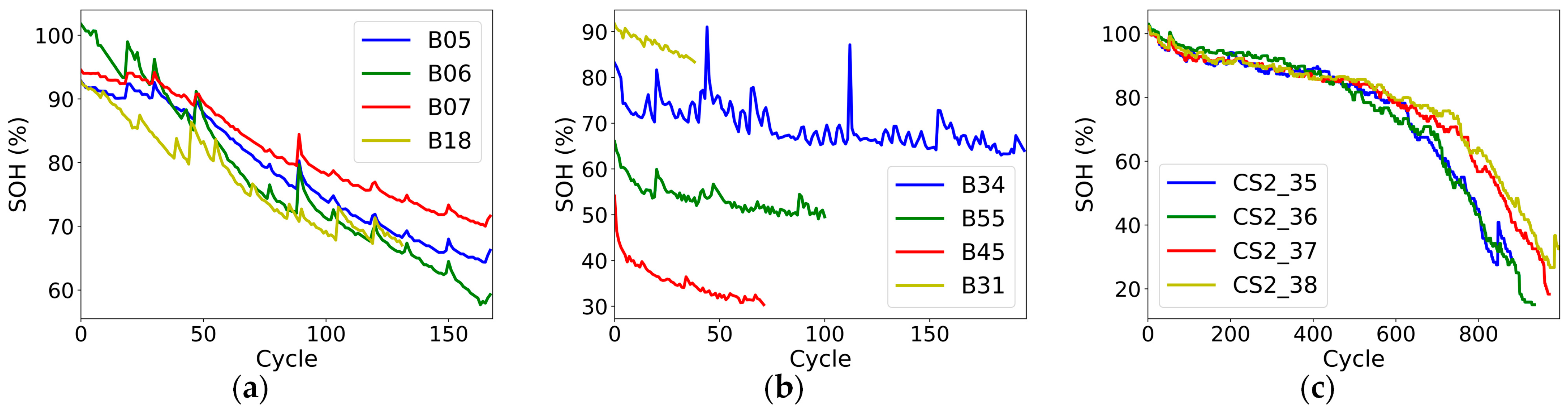
This section is based on battery degradation data from the National Aeronautics and Space Administration (NASA) Prediction Center of Excellence [29] and the Center for Advanced Life Cycle Engineering (CALCE) at the University of Maryland [30]. The rated capacity of the NASA lithium battery is 2 Ah. At room temperature of 24 °C, B05, B06, B07, and B18 are charged at a constant current (CC) of 1.5 A until the voltage rises to 4.2 V, followed by constant voltage (CV) charging until the current drops to 20 mA. They are then discharged at 2 A constant current (CC) until the voltage is 2.7 V, 2.5 V, 2.2 V, and 2.5 V, respectively. Due to the significant impact of battery operating temperature and discharge rate on battery degradation, more complex B34, B55, B45, and B31 batteries have also been used for analysis. The rated capacity of CALCE lithium battery is 1.1 Ah, with CS2_35, CS2_36, CS2_37, and CS2_38 also adopting a charging/discharging standard similar to the NASA dataset: at room temperature, CC charging is performed at 0.55 A until the voltage rises to 4.2 V, and then CV charging is performed until the current drops to 20 mA. Next, CC discharging is performed at 1.1 A until the voltage is 2.7 V. Table 1 shows the experimental conditions for each battery, and Figure 1 shows the battery capacity degradation curve.

Table 1.
Experimental conditions for each battery.
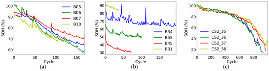
Figure 1.
Battery capacity decline curve: (a) NASA mild operating conditions; (b) NASA complex operating conditions; (c) CALCE.
2.2. Health Indicators Construction Based on Charging Curve
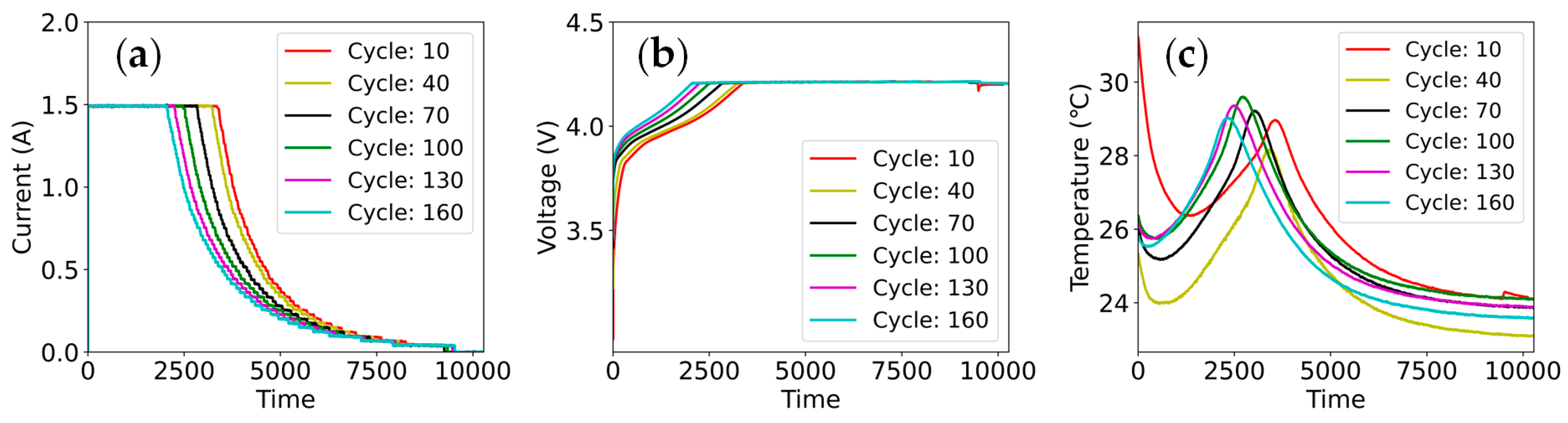
The extraction of health indicators (HIs) plays a crucial role in data-driven battery SOH estimation methods, transforming raw data into meaningful features that can be used by machine learning. Since the SOH estimation model requires the input of multidimensional features, the constructed HIs need to accurately describe the battery SOH [31]. Figure 2 shows the charging current, voltage, and temperature curves of the B07 battery over time in different cycles. From Figure 2, it can be seen that as the SOH degrades, the current, voltage, and temperature curves gradually shift to the left, while the CC charging time becomes shorter and the CV charging time becomes longer. Therefore, HIs extraction can be performed based on changes in the position of the curves.
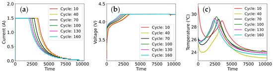
Figure 2.
Charging curves for different cycles of B07: (a) current; (b) voltage; (c) temperature.
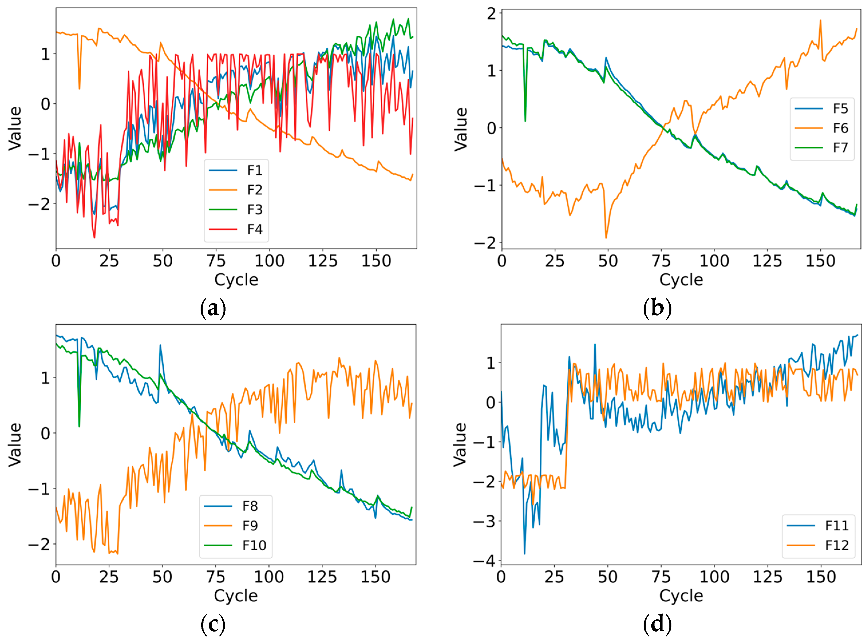
Based on the charging curves trend, 12 health indicators were extracted [32], categorized into four types: (1) time and time ratio of different charging stages: CC charging stage time F1, CV charging stage time F2, their ratio F3, and total charging time F4; (2) the integration of current curves in different charging stages over time: CC charging stage current integration F5, CV charging stage current integration F6, and total charging stage current integration F7; (3) the integration of temperature curves in different charging stages over time: CC charging stage temperature integration F8, CV charging stage temperature integration F9, and total charging stage temperature integration F10; (4) the maximum slope of the curve: the maximum slope of the charging voltage curve F11 and the maximum slope of the charging current curve F12. Taking the B07 battery as an example, these features were standardized (as shown in Equation (16) in Section 3.4) to conform to a normal distribution. The processed data curves are shown in Figure 3.

Figure 3.
Standardized health indicators of B07: (a) Type1; (b) Type2; (c) Type3; (d) Type4.
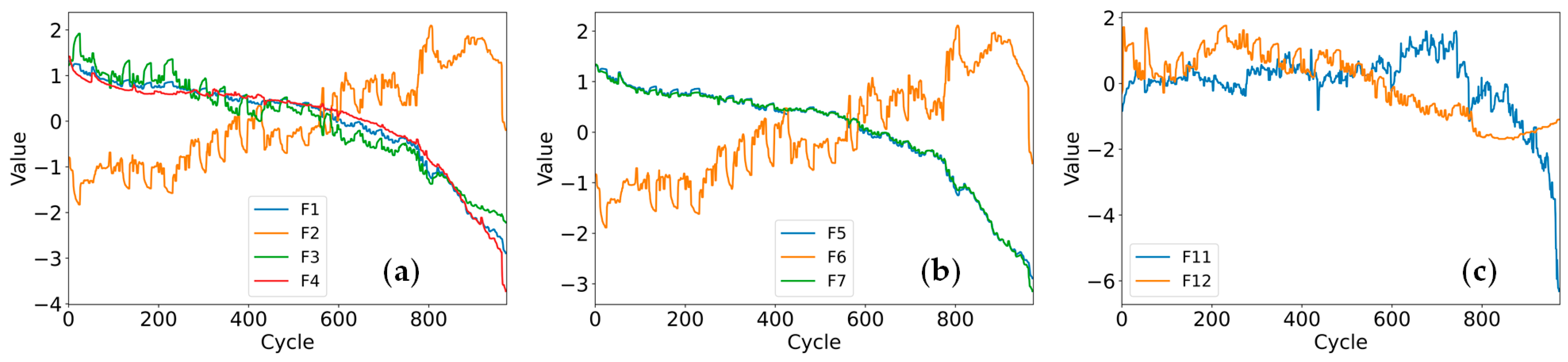
Since the CALCE dataset did not measure actual temperature, health indicators for types 1, 2, and 4 were extracted in CALCE. Taking the CS2_37 battery as an example, the processed data curves are shown in Figure 4.
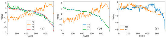
Figure 4.
Standardized health indicators of CS2_37: (a) Type1; (b) Type2; (c) Type4.
2.3. Feature Analysis Based on GRA
Figure 3 and Figure 4 illustrate the distinct changing trends of various health indicators, alongside evident autocorrelation, posing challenges in discerning the relationship between HIs and SOH. Grey relational analysis [33] is a multivariate correlation analysis method based on grey system theory and can be used to measure the degree of correlation between various variables. Employing GRA to analyze and select the pre-extracted health indicators aids in identifying crucial features, reducing data dimensions, and enhancing model performance. Table 2 outlines the steps of GRA, and Figure 5 shows the analysis results.
Table 2.
The GRA procedure.
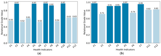
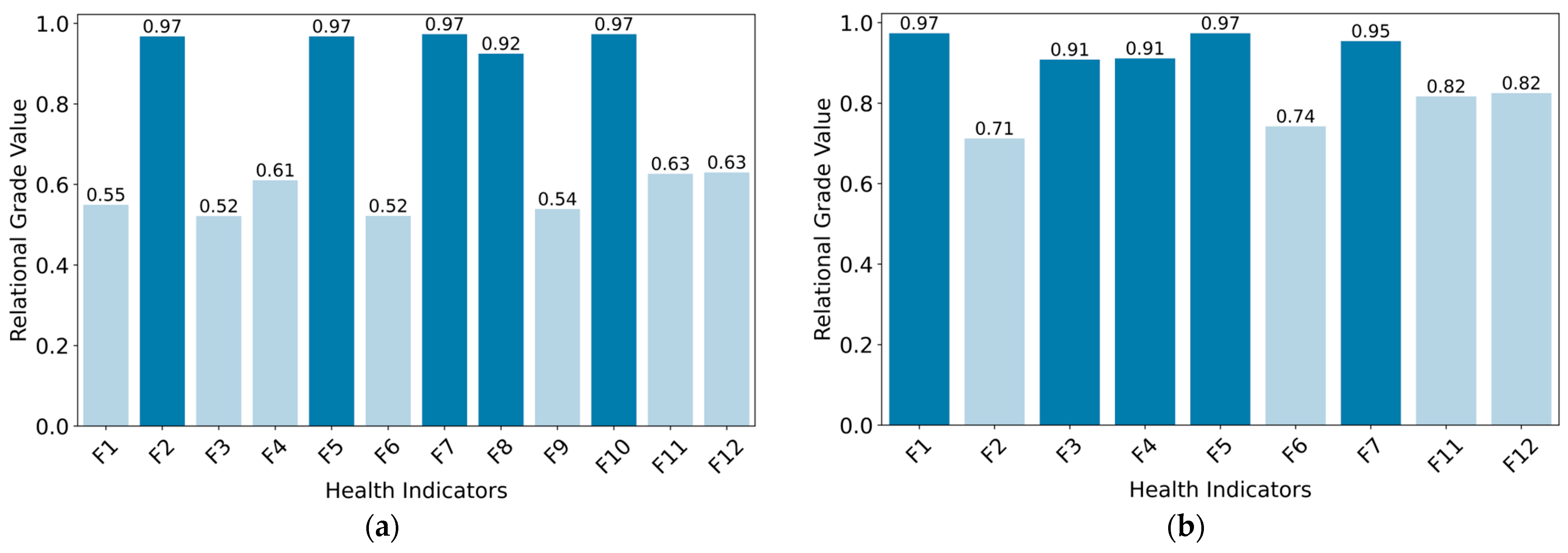
Figure 5.
Relational grade value between HIs and SOH: (a) B07; (b) CS2_37.
The relational grade value of GRA approaching 1 indicates a higher degree of correlation. As can be seen from Figure 5, the relational grade values of F2, F5, F7, F8, and F10 of B07, and F1, F3, F4, F5, and F7 of CS2_37 all surpass 0.9, while the remaining values are either less than or equal to 0.82. Consequently, these health indicators were chosen for estimating the SOH of B07 and CS2_37.
3. SOH Estimation Model Based on Fennec Fox Optimization Algorithm–Mixed Extreme Learning Machine
3.1. Extreme Learning Machine
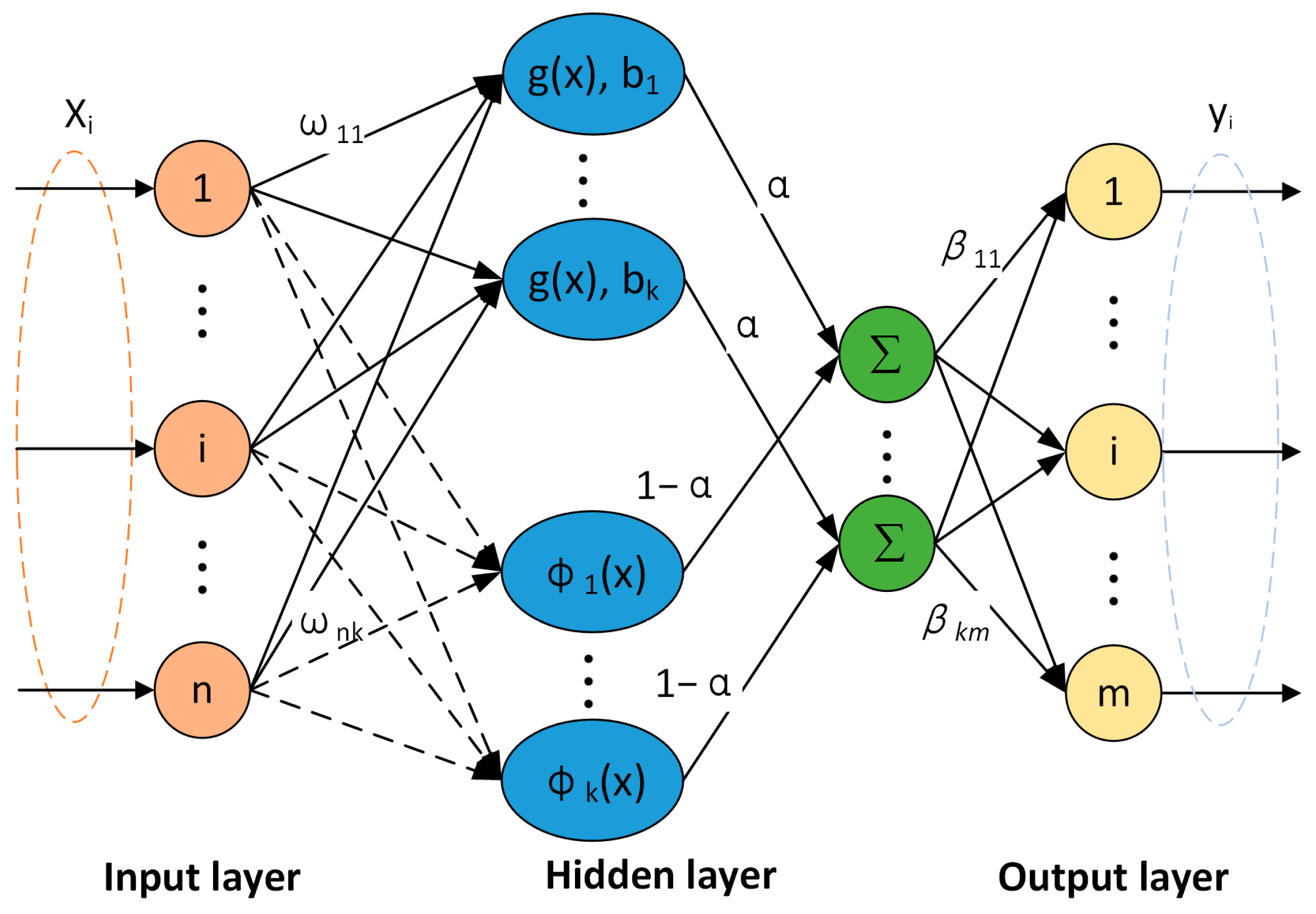
Extreme learning machine (ELM) is a type of single hidden layer feedforward neural network (SLFNN) algorithm [34]. It comprises an input layer, a hidden layer, and an output layer, as depicted in Figure 6. During training, only the weights and biases connecting the input layer and the hidden layer require random initialization, while the weights of the output layer can be computed directly without iterative optimization such as backpropagation. ELM demonstrates the ability to swiftly handle large-scale aging data with simple hyperparameter configurations, enabling precise real-time estimation of SOH even with limited data.
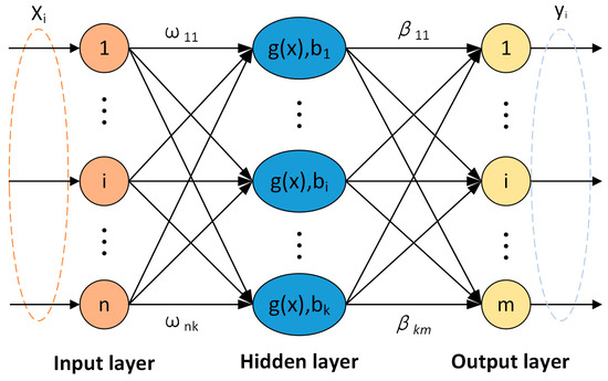
Figure 6.
The network structure of ELM.
Given a training set of N samples, , where is the input for the i-th sample, is the i-th sample label. The output of an ELM with K hidden nodes can be defined as follows:
where is the combined weight between the j-th hidden layer neuron and the input layer, is the bias of the j-th hidden layer neuron, is the activation function, and represents the combined weight between the j-th hidden layer neuron and the output layer. Equation (2) can be expressed in matrix form as follows:
where , and
Neural networks adapt the weights and biases between neurons according to training data, while in the ELM training process, since the input weights of hidden layers and the bias are randomly assigned, the output matrix of the hidden layer can be derived. The solving process can be transformed into a linear parameter solving process, wherein only the output weights need to be calculated, based on Equation (3), and the solving process can be defined as follows:
where is the Moore–Penrose generalized inverse matrix of .
3.2. Mixed Extreme Learning Machine
The extreme learning machine based on the radial basis function (ELM-RBF) utilizes RBF as the basis function in the hidden layer. This allows for better handling of nonlinear problems while maintaining the rapid training characteristics of ELM [35]. The output of the j-th hidden layer neuron can be represented as follows:
where the center of the radial basis function and radius are randomly initialized, and the output of ELM-RBF with K hidden nodes can be defined as follows:
To better capture the characteristics of the input data, this paper integrates ELM and ELM-RBF to formulate a mixed hidden layer neuron output. This is achieved by employing both the sigmoid activation function and RBF, with the weighted output controlled by a mixed parameter , resulting in the mixed extreme learning machine (MELM). The output of the j-th hidden layer neuron can be represented as follows:
where represents the sigmoid activation function, is a mixed parameter utilized to modulate the contribution of the two parts, with a value ranging between 0 and 1. Following the same procedure as ELM, only the output weight needs to be solved; the network structure of MELM is presented in Figure 7.

Figure 7.
The network structure of MELM.
3.3. Fennec Fox Optimization Algorithm
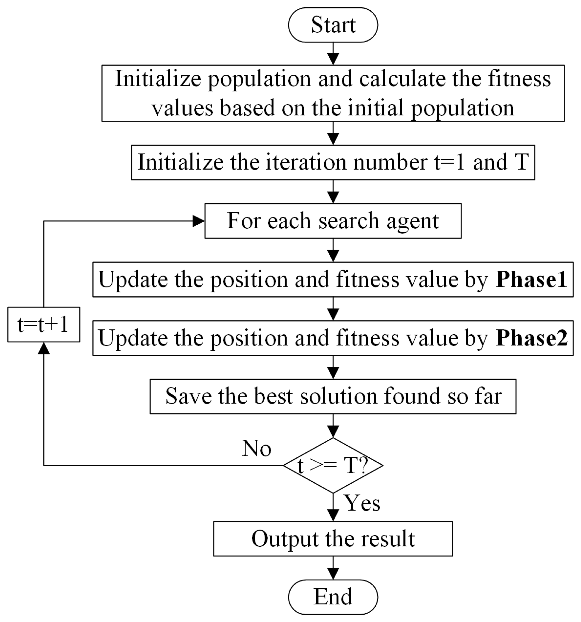
The fennec fox optimization algorithm (FFA) is a novel swarm intelligence algorithm inspired by the predatory and evasion behaviors of the fennec fox population in nature [36]. FFA solves optimization problems by simulating these two behaviors. The algorithm mainly consists of two stages: digging prey behavior in the sand and escaping predators.
- (1)
- Phase1: Digging prey behavior in the sand (local search).
When hunting, the fennec fox uses its sensitive hearing to detect the position of prey under the sand, excavate, and capture its prey. Simulating this behavior can improve the local search ability of FFA and bring it closer to the global optimal solution. It is assumed there are N fennec foxes, where the position of the i-th fox is denoted as , and the fitness value in this position is . A local search is performed on the neighborhood with as the center and radius R. The first phase position update model is as follows:
where represents the position of the i-th fennec fox based on the first phase update, represents the position of its j-th dimension, and is the fitness value of . is the neighborhood radius of , is the iteration counter, represents the total number of iterations, is a random number in the interval [0, 1], and is a constant set to 0.2.
- (2)
- Phase2: Escaping predators (global search).
When encountering the pursuit of predators, the fennec fox can escape the pursuit of predators with its remarkable speed and abrupt changes in direction. The escape strategy of the fennec fox serves as the foundation for global searching. This escape strategy enhances the exploration ability of FFA, enabling it to skip out of the local optimal area and identify the global optimal area. The second phase position update model is as follows:
where represents the target position of the i-th fennec fox escaping, denotes its position in the j-th dimension, and is the fitness value at that position. is the position of the i-th fennec fox based on the second phase update, denotes its position in the j-th dimension, and is the fitness value at that position. is a random number between [0, 1], and is a random number selected from the set {1, 2}. Based on the above behaviors of the fennec fox population, the FFA flowchart is shown in Figure 8.
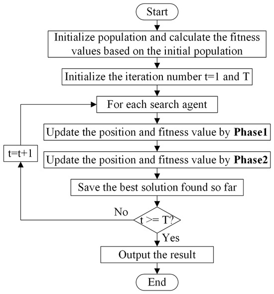
Figure 8.
FFA flowchart.
3.4. FFA-MELM
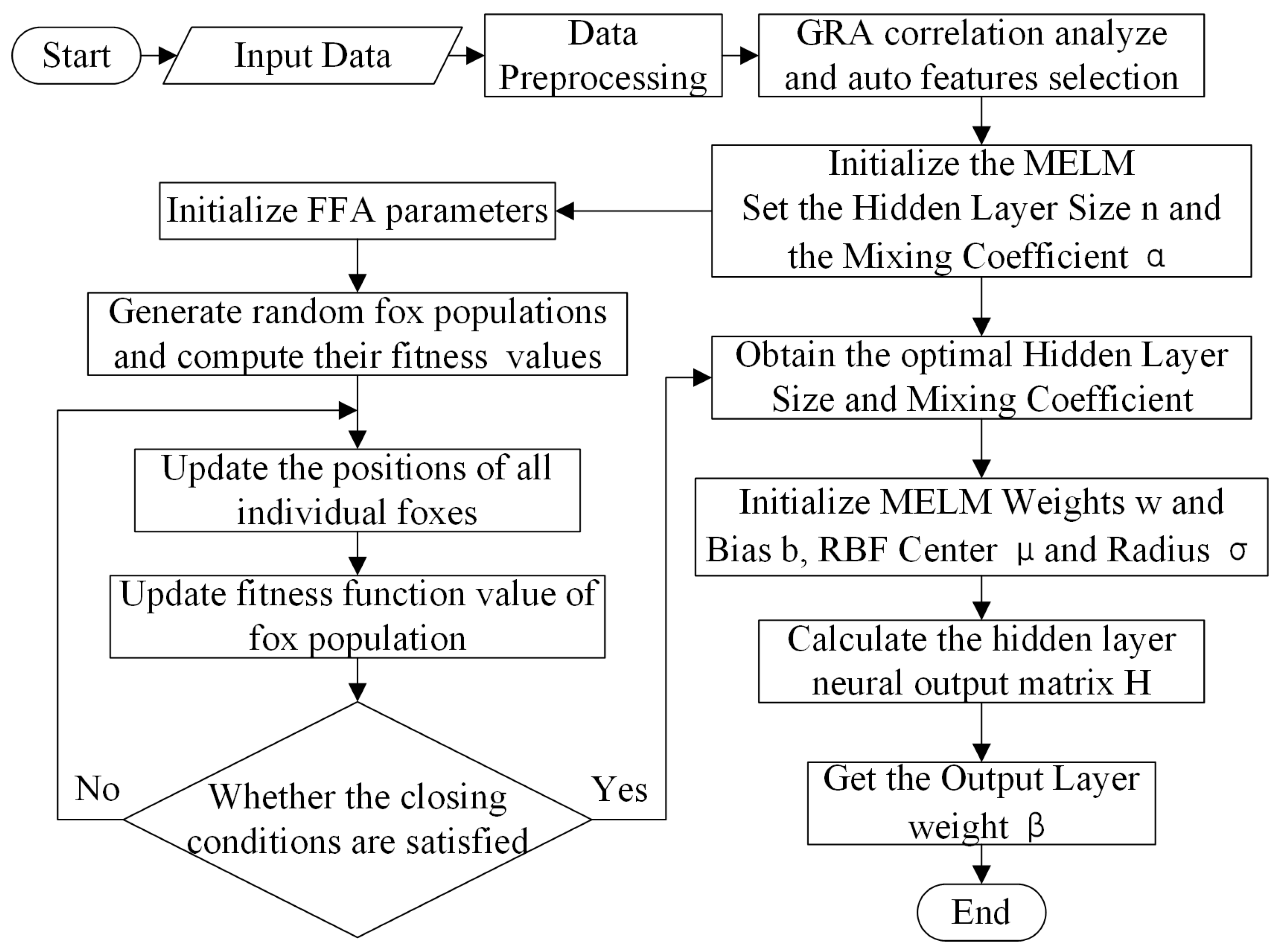
The number of hidden layer neurons n and the mixed parameter are critical parameters affecting the performance of MELM. Insufficient neurons can result in underfitting and inability to capture complex data relationships, while excessive numbers may lead to overfitting, increasing the training time. The value of also impacts the accuracy and generalization of MELM. FFA is a novel global optimization algorithm that offers distinct advantages in optimizing MELM hyperparameters, thus effectively improving model performance. The process of the FFA-MELM is depicted in Figure 9.
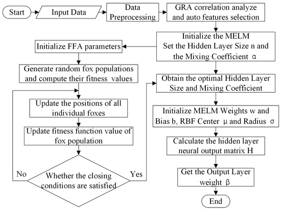
Figure 9.
FFA-MELM flowchart.
The steps of FFA-MELM are listed below:
- (1)
- Data preprocessing: Standardize the features of the sample data according to Equation (16), ensuring that data conform to the standard normal distribution N(0, 1). The preprocessed data can then be divided into training and test samples.
- (2)
- Feature analysis and automatic feature selection: The features of the sample data are analyzed using GRA to determine their importance. The top K features are then selected as inputs for the SOH estimation model.
- (3)
- Set the model parameters: In the model, the number of fennec fox populations is set to 100, the position dimension is set to 2, the total number of iterations is set to 50, the hidden layer neurons n in MELM are set to [2, 50], the mixed parameter is set to (0, 1), and the optimized fitness function is defined as follows:where and are the estimated and actual values of SOH for the i-th training sample, respectively, and N is the number of training samples.
- (4)
- Random initialization of population position: Each fennec fox corresponds to a set of spatial position vectors (n, ). Randomly initialize the position of the fennec fox population based on the value range of n and defined in step 3.
- (5)
- MELM hyperparameter optimization: Utilize FFA to optimize the number of hidden layer neurons and mixed parameters of MELM.
- (6)
- Set termination condition: If the total number of iterations is reached, terminate the algorithm and output the global optimal position parameters (nbest, αbest).
- (7)
- Establish the optimal model: Based on the parameters (nbest, αbest), establish the final MELM estimation model and output the estimated SOH.
4. Experiment and Analysis
4.1. SOH Estimation Accuracy Experiment
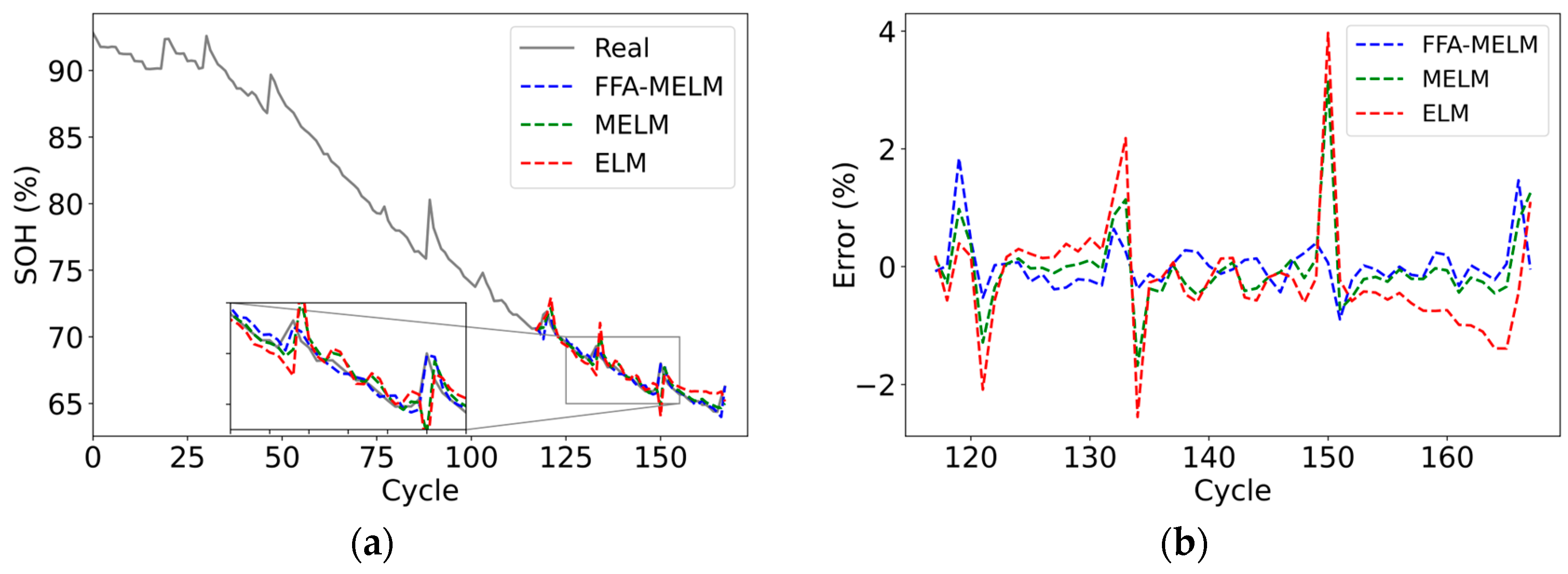
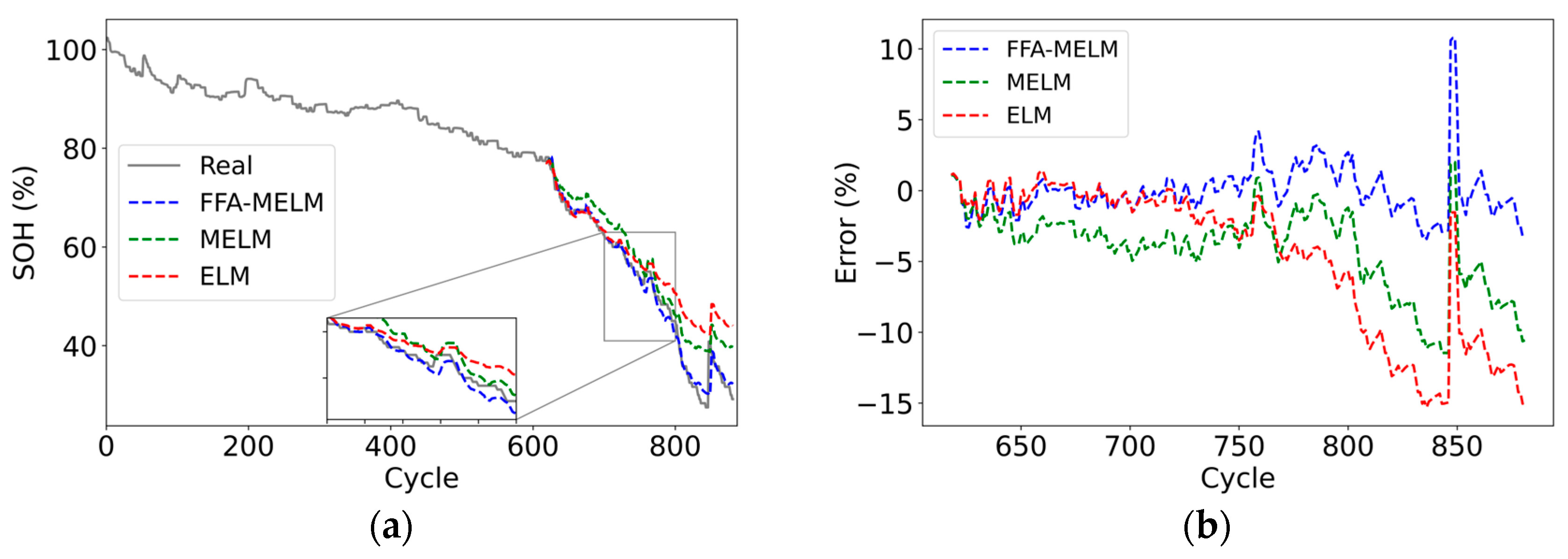
B05, B06, B07, B18, B34, B55, B45, and B31 from the NASA dataset were selected as experimental subjects. The first 70% of the battery cycle data was used as training data, and the remaining data were used for testing to assess the accuracy and reliability of the proposed method. The results and errors of SOH estimation for B05, B06, B07, and B18 are shown in Figure 10.
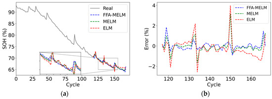
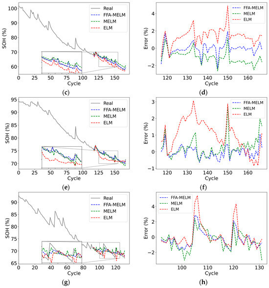
Figure 10.
SOH estimation experiments of different methods under mild operating conditions. Estimation results: (a) B05; (c) B06; (e) B07; (g) B18. The estimation error of the test data: (b) B05; (d) B06; (f) B07; (h) B18.
Figure 10 shows that the FFA-MELM method significantly outperforms MELM and ELM in estimating the SOH decay curve of B05, B06, B07, and B18 under mild operating conditions, with an estimation error basically within 1%. Furthermore, it also achieves a satisfactory curve-fitting effect in the capacity regeneration area.
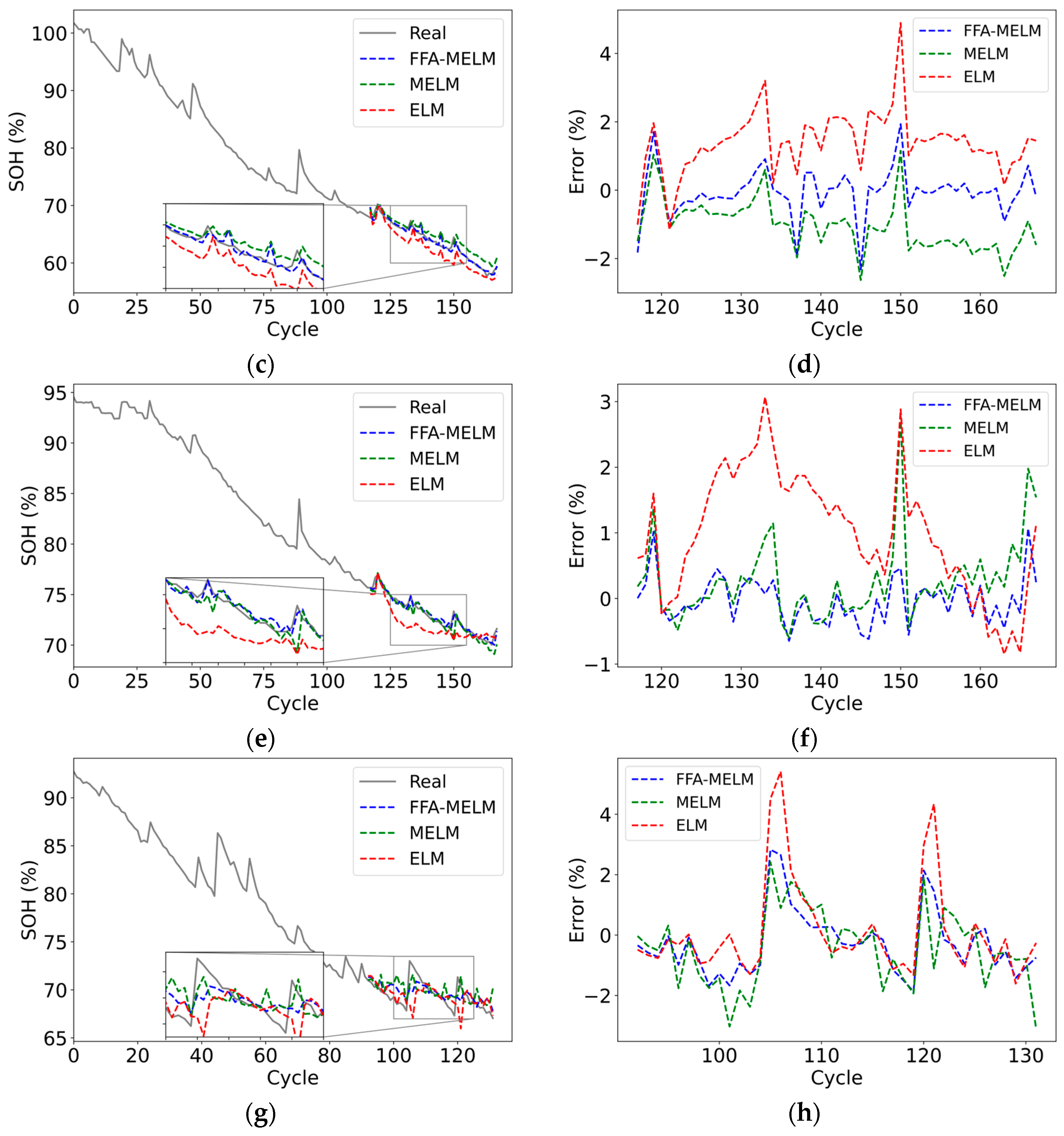
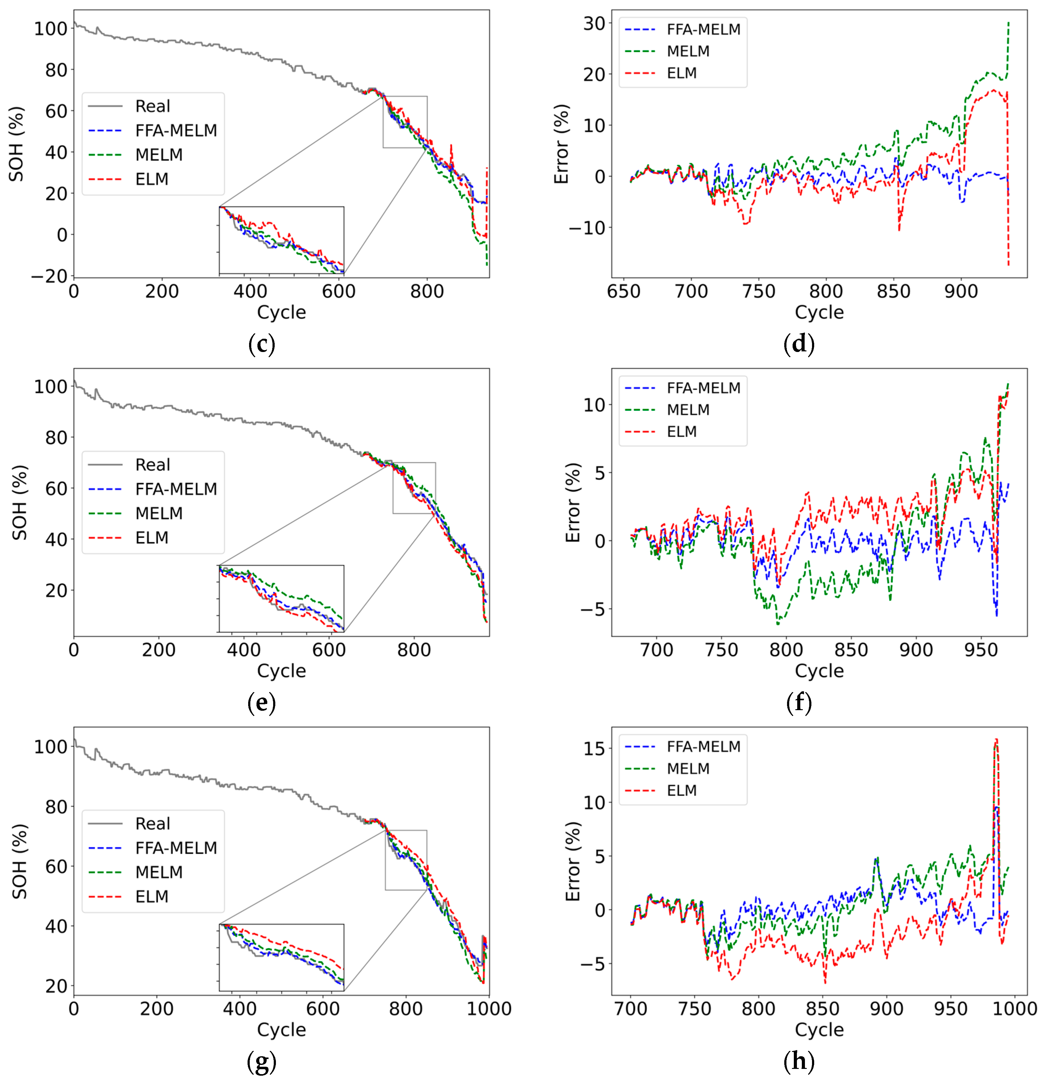
For batteries subjected to complex operating conditions, temperature variations can influence the chemical reaction rate inside the battery, potentially leading to damage to the materials within. High discharge rates result in increased heat generation inside the battery, leading to the thickening of the SEI film and accelerated battery aging. The SOH estimation experiments of B34, B55, B45, and B31 under complex operating conditions are shown in Figure 11.
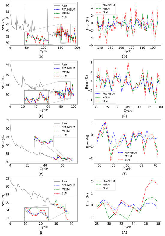
Figure 11.
SOH estimation experiments of different methods under complex operating conditions. Estimation results: (a) B34; (c) B55; (e) B45; (g) B31. Estimation error of the test data: (b) B34; (d) B55; (f) B45; (h) B31.
Figure 11 indicates that B34 and B55 display increased nonlinearity under complex operating conditions, characterized by larger fluctuations in the capacity decay curve. The ELM model estimation results prove inaccurate; however, FFA-MELM accurately captures the SOH decay trend with maximum estimation errors within 2% and 3%, respectively, exhibiting the best fitting effect. Regarding B45 operating at low temperatures and slower discharge rates and B31 operating at high temperatures and faster discharge rates, FFA-MELM also demonstrates superior performance, with maximum errors within 1%.
To comprehensively evaluate the SOH estimation performance of the proposed method, three different indicators were employed in the experiment, namely mean absolute error (MAE), root mean square error (RMSE), and mean absolute percentage error (MAPE). The model’s smaller MAE and RMSE indicate fewer prediction errors and a better fit to the actual SOH. To address the sensitivity of RMSE to outliers, MAPE is utilized for auxiliary evaluation. The equations for these indicators are as follows:
where and represent the actual and predicted values of the i-th sample, respectively, and N is the number of samples. Table 3 presents the performance metrics for SOH estimation.
Table 3.
Performance metrics of different methods.
Table 3 shows that FFA-MELM surpasses MELM and ELM under both mild and complex operating conditions. For eight batteries, the average MAE of FFA-MELM is 0.55%, which is 0.31% and 0.58% lower than MELM and ELM, respectively. Additionally, the average RMSE is 0.71%, representing a decrease of 0.37% and 0.76% compared to MELM and ELM, respectively. Moreover, the average MAPE is 0.98%, showcasing a reduction of 0.5% and 0.89% in comparison to MELM and ELM, respectively. Although the evaluation indicators for B34 and B55 batteries operating under complex conditions are slightly higher than those of other batteries, the estimation errors remain within a stable range.
Based on the analysis above, it is evident that the proposed FFA-MELM estimation method effectively addresses the issues of inadequate fitting ability and challenges in the hyperparameter optimization of ELM. The method accurately captures the declining trend of battery SOH and adapts well to the phenomenon of capacity regeneration during aging. FFA-MELM achieves more precise SOH estimation compared to ELM and demonstrates robust adaptability and stability under complex operating conditions.
4.2. SOH Estimation Experiments with Different Starting Points for Testing
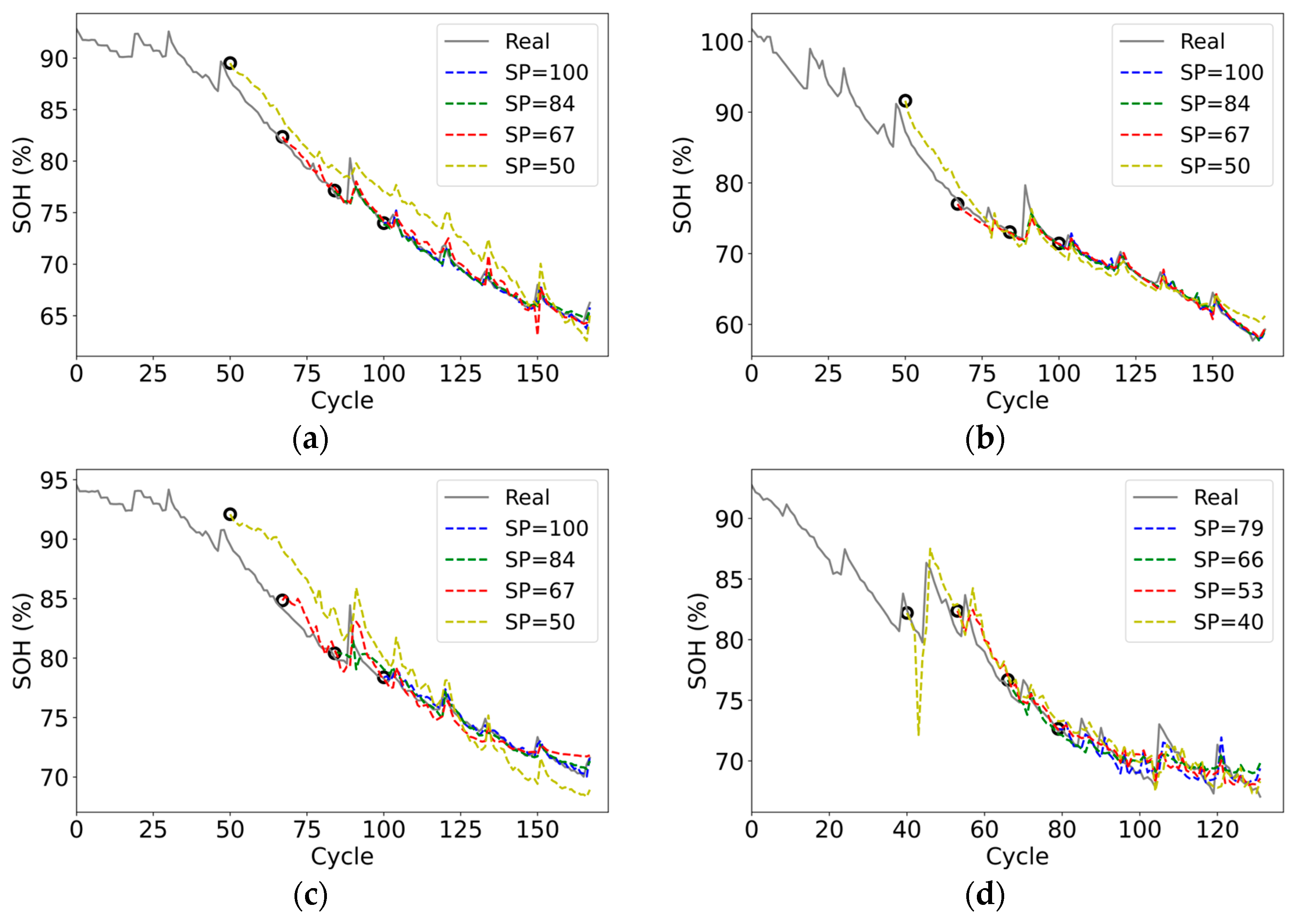
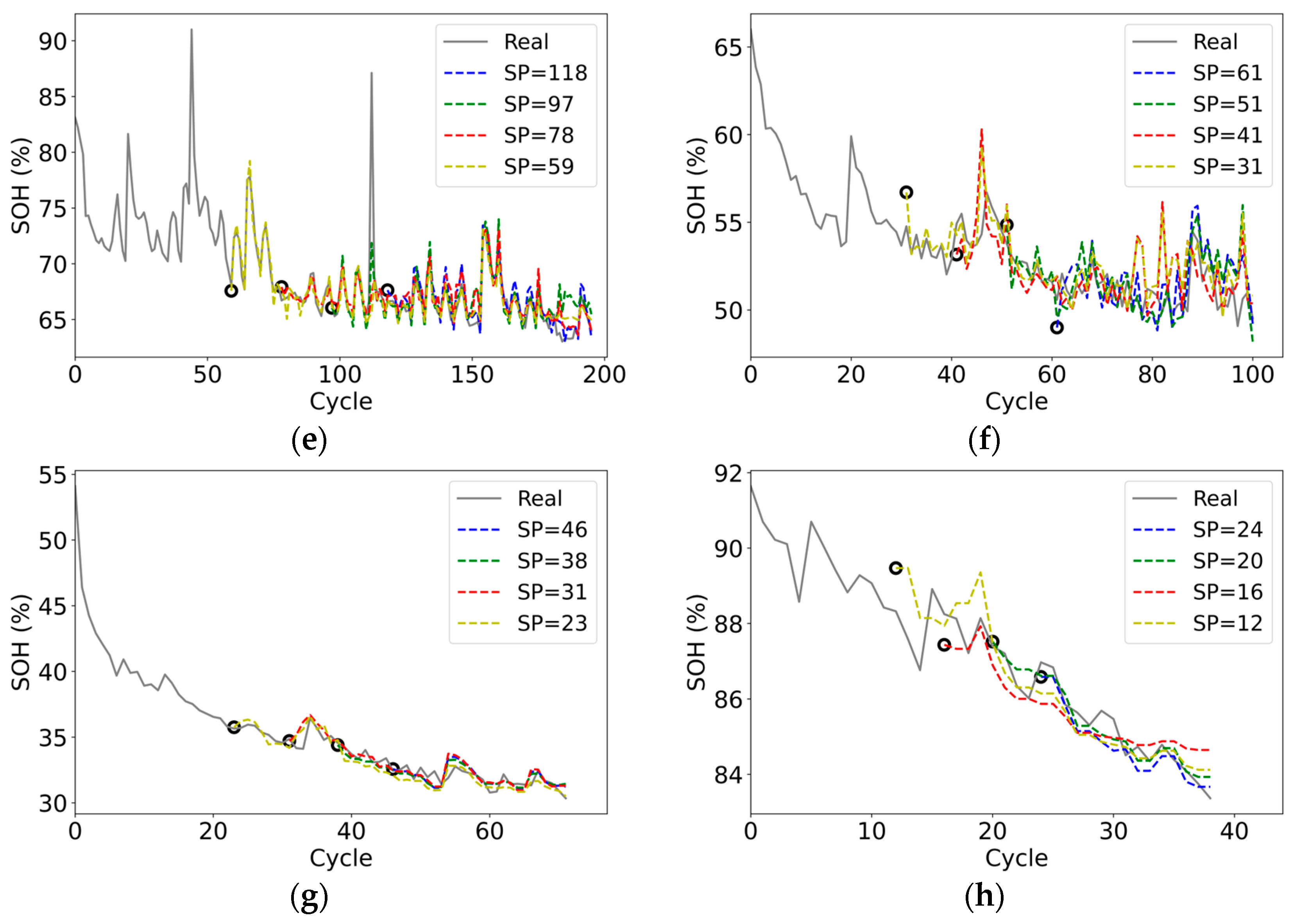
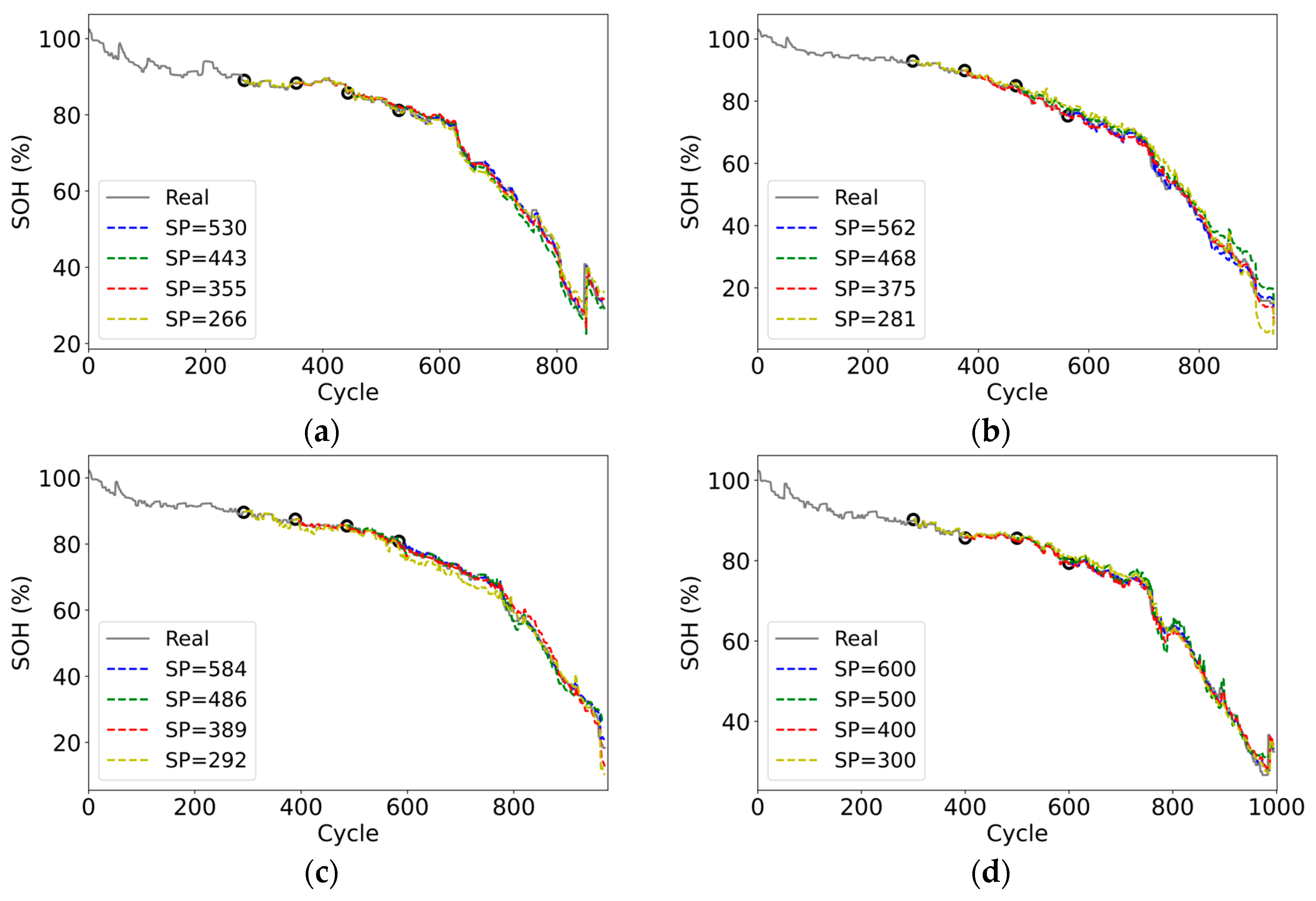
To investigate the impact of the training set size on model estimation accuracy, batteries B05, B06, B07, B18, B34, B55, B45, and B31 from the NASA dataset were selected for experimentation. The first 60%, 50%, 40%, and 30% of the battery cycle data were utilized as the training data, and the remaining data as the testing data. The experiment to estimate SOH begins from different starting points (SP) to verify the robustness of the proposed method. The estimation results are shown in Figure 12, and the performance metrics are presented in Table 4.
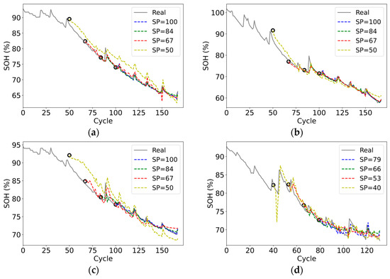
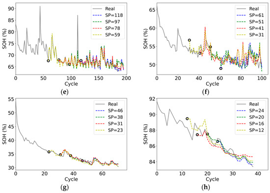
Figure 12.
SOH estimation results at different starting test points: (a) B05; (b) B06; (c) B07; (d) B18; (e) B34; (f) B55; (g) B45; (h) B31.
Table 4.
Performance metrics of different starting points for testing.
As shown in Figure 12, the proposed method accurately fits the capacity decline curve of eight batteries when the training data comprise 40% or more of the total data. Even with only 30% training data, the proposed method is still able to fit the trend of capacity decline well. However, there are relatively large errors observed in the capacity regeneration and end regions of the decay curve. This limitation may stem from the small amount of training data available, hindering the model’s ability to accurately capture strong nonlinearities and large fluctuations. From Table 4, it is evident that under mild operating conditions and with 30% training data, the proposed method can still adequately reflect the trend of battery capacity decline, despite a relatively large SOH estimation error. When the volume of training data is 40% or greater, the average MAE, RMSE, and MAPE are 0.58%, 0.89%, and 0.81%, respectively. These values are close to the performance achieved with 70% of the data volume.
From Table 4, it can be seen that even under complex operating conditions and with reduced training data, the SOH estimation error remains relatively stable. The average MAE, RMSE, and MAPE are 0.77%, 1.14%, and 1.43%, respectively, indicating excellent SOH estimation. It should be noted that for B45 and B31 batteries, FFA-MELM exhibits performance comparable to that achieved with 60% of the training data, even when the training data volume is as low as 30%. This further confirms the adaptability and robustness of the proposed method.
Based on the above discussion, the proposed FFA-MELM method demonstrates high accuracy, good adaptability, and robustness for estimating battery SOH. Furthermore, it reduces the demand for training data. Even under complex operating conditions and with limited training data, the model can still accurately reflect the overall SOH trend. As more training data are collected, the performance of the estimation model will gradually improve.
4.3. Adaptability Experiments for Different Battery Types
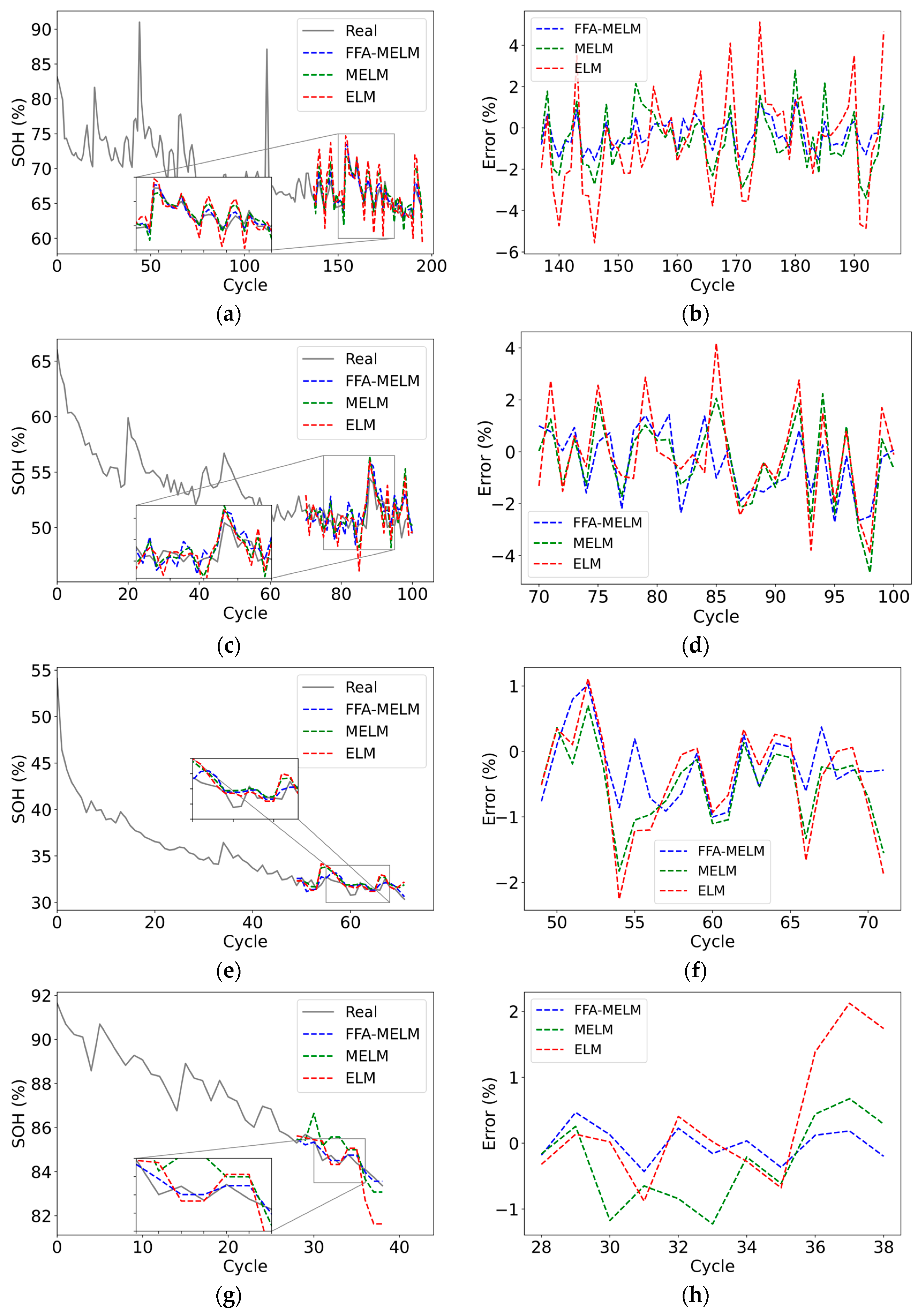
To assess the adaptability and robustness of the proposed method across different types of batteries, CS2_35, CS2_36, CS2_37, and CS2_38 from CALCE have been selected for the experiments. The experimental setup is identical to that described in Section 4.1. Figure 13 displays the SOH estimation results and errors, and Table 5 presents the performance metrics for different methods.
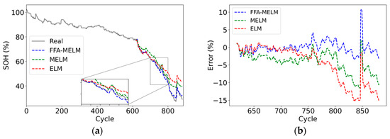
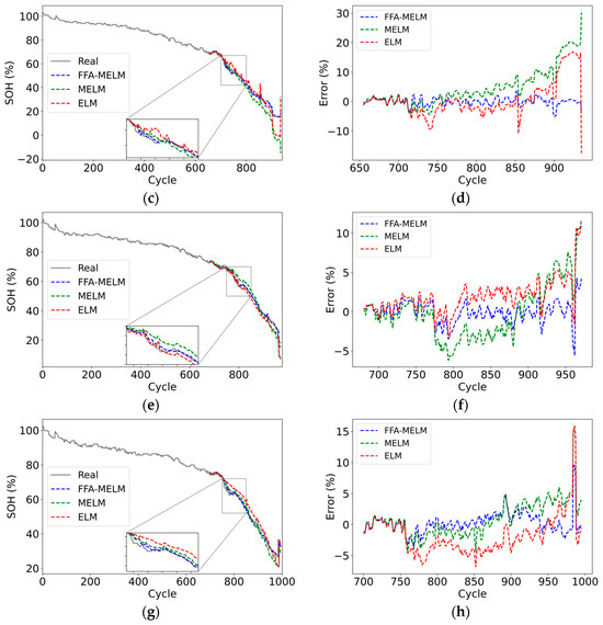
Figure 13.
SOH estimation experiments of different methods for CALCE. Estimation results: (a) CS2_35; (c) CS2_36; (e) CS2_37; (g) CS2_38. Estimation error of the test data: (b) CS2_35; (d) CS2_36; (f) CS2_37; (h) CS2_38.
Table 5.
Performance metrics of different methods for CALCE.
Figure 13 shows that all three methods exhibit a good fitting effect, attributed to the slow capacity decline curve of the CALCE dataset in the early stage. The estimation errors remain relatively stable. However, during the later stage of rapid decline in SOH, the FFA-MELM method provides a superior fit for the SOH decline curve compared to MELM and ELM. This is particularly evident in the area of capacity regeneration, where the proposed method also displays the smallest estimation error. As shown in Table 5, ELM performs poorly on various types of batteries. Conversely, FFA-MELM achieves lower MAE, RMSE, and MAPE values for all four batteries, each below 1.3%, 1.9%, and 2.8%, respectively.
The experimental setup for SOH estimation experiments is the same as described in Section 4.2, with different starting points. The experimental results are shown in Figure 14, and the performance metrics are presented in Table 6.
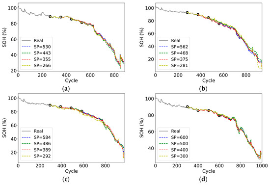
Figure 14.
SOH estimation results at different starting test points for CALCE: (a) CS2_35; (b) CS2_36; (c) CS2_37; (d) CS2_38.
Table 6.
Performance metrics of different starting points for testing for CALCE.
Figure 14 shows that even with reduced training data, the proposed method can still fit the battery capacity degradation trend well with high estimation accuracy. However, a notable error is observed in the final stage of the curve, possibly due to the highly unstable battery performance during this phase.
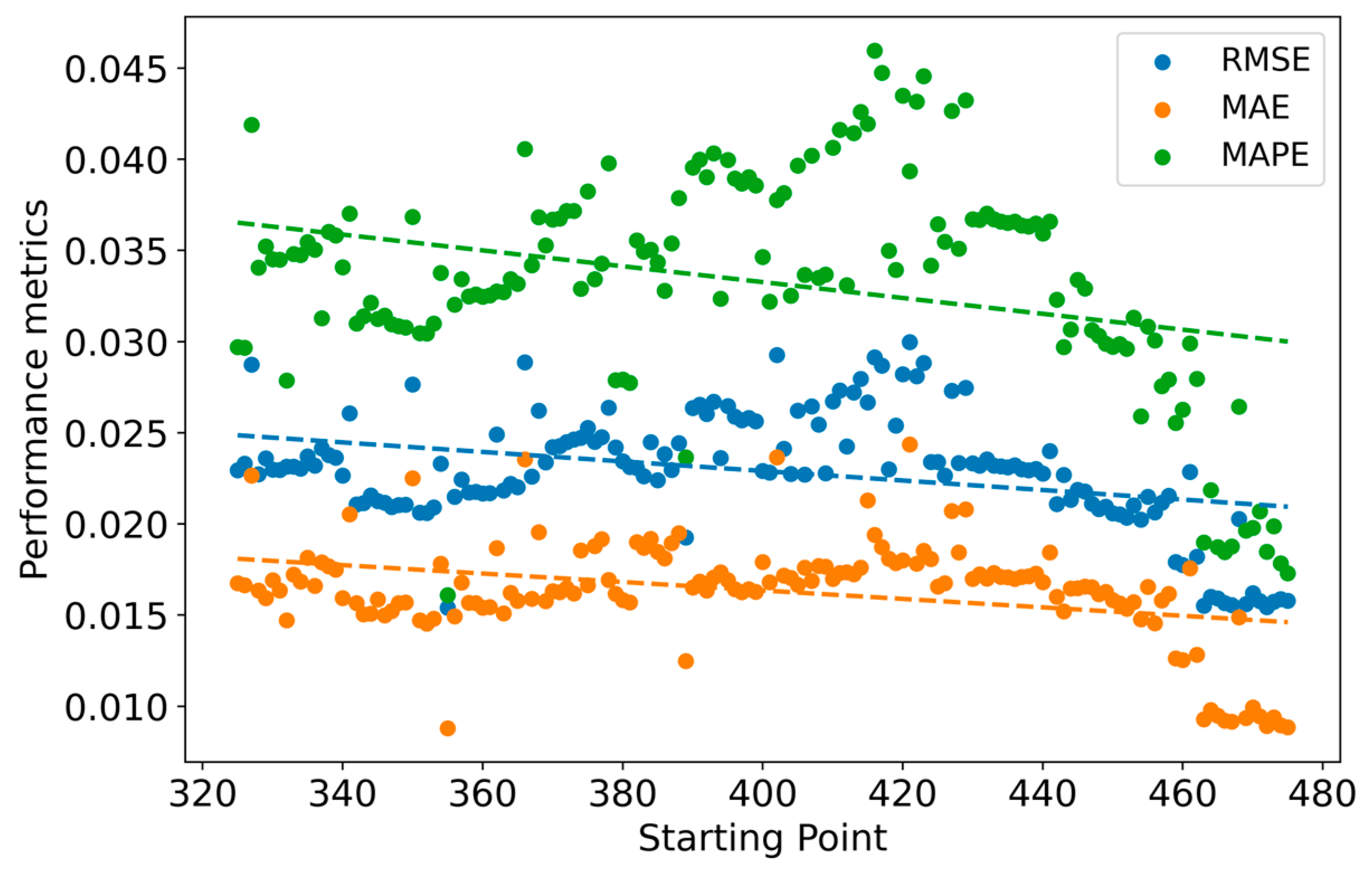
Table 6 demonstrates that even with reduced training data, FFA-MELM can effectively capture crucial information regarding the decline in capacity from limited data. The proposed method can robustly estimate SOH, as indicated by the average MAE, RMSE, and MAPE values of 1.25%, 1.8%, and 2.82%, respectively. It is noteworthy to mention that reducing the training data from 50% to 40% results in a reduction in estimation error. To delve deeper into this matter, a refinement experiment was conducted using CS2_35 as an example. The experiment was carried out on approximately 40–50% of the data (355 and 443 cycles), with 150 experiments conducted at different starting points ranging from 325 to 475 cycles. The results of the experiment are presented in Figure 15.
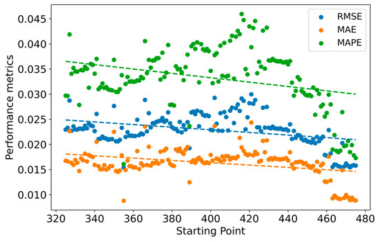
Figure 15.
Performance metrics of different starting points ranging from 325 to 475 cycles for CS2_35.
Figure 15 shows the first-order fitting lines (as shown in Equation (21)) for the performance metrics, which indicates a decreasing trend. This suggests that the error diminishes as the amount of data increases. The larger errors observed in individual starting estimation points may be attributed to the fact that battery aging is a nonlinear system involving complex material, chemical, and physical mechanisms. Furthermore, the fluctuation range of the error mostly remains within 1%, indicating that the proposed method can obtain stable estimation results at different starting cycle points.
where represents the fitting line, and and are the slope and intercept, respectively.
5. Conclusions
To enhance the accuracy of SOH estimation for lithium batteries, this paper proposes an SOH estimation method based on FFA-MELM. Firstly, health indicators were extracted by analyzing the battery charging curve. The correlation between health indicators and SOH was analyzed using GRA. The features highly correlated with battery SOH degradation were selected as model inputs, with SOH as the output. To address the issues of low estimation accuracy and weak generalization in ELM, MELM was proposed in combination with ELM-RBF. To solve the hyperparameter optimization problem of MELM, FFA was utilized to optimize the number of hidden layer neurons and mixed parameters of MELM, and an SOH estimation model was established for FFA-MELM. Finally, 12 batteries from NASA and CALCE battery datasets were employed for SOH estimation experiments. The experimental results demonstrate that the proposed method effectively improves the accuracy of SOH estimation compared to other methods such as MELM and ELM. Additionally, it maintains stable accuracy across different types of batteries, complex operating conditions, and limited training data.
In this study, batteries from the NASA and CALCE datasets were selected for the experiments. However, it did not account for the capacity degradation of lithium batteries under real operating conditions of electric vehicles. To enhance the accuracy and generalizability of SOH estimation for lithium batteries, future work will concentrate on two aspects: (1) creating straightforward and effective feature engineering techniques to reduce reliance on data integrity and computational complexity; (2) developing online SOH estimation algorithms based on real vehicle data to improve the computational efficiency of SOH estimation.
Author Contributions
Conceptualization, C.S., W.Q. and Z.Y.; methodology, C.S.; software, C.S.; validation, C.S., W.Q. and Z.Y.; formal analysis, C.S.; investigation, C.S.; resources, C.S.; writing original draft preparation, C.S.; writing—review and editing, C.S. and Z.Y.; visualization, C.S.; supervision, W.Q.; project administration, W.Q. All authors have read and agreed to the published version of the manuscript.
Funding
This work was supported by the Key R&D Program of Jiangsu Province under Grant BE2023010-3 and the Jiangsu Modern Agricultural Industry Single Technology Research and Development project under Grant CX(23)3120.
Data Availability Statement
The data used in this paper are from the NASA Battery Aging Dataset and the CALCE battery dataset of CS2 cells.
Conflicts of Interest
The authors declare no conflicts of interest.
References
- Hu, X.; Zhang, K.; Liu, K.; Lin, X.; Dey, S.; Onori, S. Advanced Fault Diagnosis for Lithium-Ion Battery Systems: A Review of Fault Mechanisms, Fault Features, and Diagnosis Procedures. IEEE Ind. Electron. Mag. 2020, 14, 65–91. [Google Scholar] [CrossRef]
- Smarsly, K.; Law, K.H. Decentralized Fault Detection and Isolation in Wireless Structural Health Monitoring Systems Using Analytical Redundancy. Adv. Eng. Softw. 2014, 73, 1–10. [Google Scholar] [CrossRef]
- Rauf, H.; Khalid, M.; Arshad, N. Machine Learning in State of Health and Remaining Useful Life Estimation: Theoretical and Technological Development in Battery Degradation Modelling. Renew. Sustain. Energy Rev. 2022, 156, 111903. [Google Scholar] [CrossRef]
- Vennam, G.; Sahoo, A.; Ahmed, S. A Survey on Lithium-Ion Battery Internal and External Degradation Modeling and State of Health Estimation. J. Energy Storage 2022, 52, 104720. [Google Scholar] [CrossRef]
- Lipu, M.S.H.; Ansari, S.; Miah, M.S.; Meraj, S.T.; Hasan, K.; Shihavuddin, A.S.M.; Hannan, M.A.; Muttaqi, K.M.; Hussain, A. Deep Learning Enabled State of Charge, State of Health and Remaining Useful Life Estimation for Smart Battery Management System: Methods, Implementations, Issues and Prospects. J. Energy Storage 2022, 55, 105752. [Google Scholar] [CrossRef]
- Li, Q.; Li, D.; Zhao, K.; Wang, L.; Wang, K. State of Health Estimation of Lithium-Ion Battery Based on Improved Ant Lion Optimization and Support Vector Regression. J. Energy Storage 2022, 50, 104215. [Google Scholar] [CrossRef]
- Xiong, R.; Li, L.; Tian, J. Towards a Smarter Battery Management System: A Critical Review on Battery State of Health Monitoring Methods. J. Power Sources 2018, 405, 18–29. [Google Scholar] [CrossRef]
- Yao, L.; Xu, S.; Tang, A.; Zhou, F.; Hou, J.; Xiao, Y.; Fu, Z. A Review of Lithium-Ion Battery State of Health Estimation and Prediction Methods. World Electr. Veh. J. 2021, 12, 113. [Google Scholar] [CrossRef]
- Wang, Y.; Tian, J.; Sun, Z.; Wang, L.; Chen, Z. A Comprehensive Review of Battery Modeling and State Estimation Approaches for Advanced Battery Management Systems. Renew. Sustain. Energy Rev. 2020, 131, 110015. [Google Scholar] [CrossRef]
- Bi, Y.; Yin, Y.; Choe, S.Y. Online State of Health and Aging Parameter Estimation Using a Physics-Based Life Model with a Particle Filter. J. Power Sources 2020, 476, 228655. [Google Scholar] [CrossRef]
- Gao, Y.; Liu, K.; Zhu, C.; Zhang, X.; Zhang, D. Co-Estimation of State-of-Charge and State-of- Health for Lithium-Ion Batteries Using an Enhanced Electrochemical Model. IEEE Trans. Ind. Electron. 2022, 69, 2684–2696. [Google Scholar] [CrossRef]
- Li, J.; Adewuyi, K.; Yagin, N.L.; Landers, R.; Park, J. A Single Particle Model with Chemical/Mechanical Degradation Physics for Lithium Ion Battery State of Health (SOH) Estimation. Appl. Energy 2018, 212, 1178–1190. [Google Scholar] [CrossRef]
- Tran, M.-K.; Mathew, M.; Janhunen, S.; Panchal, S.; Raahemifar, K.; Fraser, R.; Fowler, M. A Comprehensive Equivalent Circuit Model for Lithium-Ion Batteries, Incorporating the Effects of State of Health, State of Charge, and Temperature on Model Parameters. J. Energy Storage 2021, 43, 103252. [Google Scholar] [CrossRef]
- Sihvo, J.; Roinila, T.; Stroe, D.I. SOH Analysis of Li-Ion Battery Based on ECM Parameters and Broadband Impedance Measurements. In Proceedings of the the 46th Annual Conference of the IEEE Industrial Electronics Society (IECON), Singapore, 18–21 October 2020. [Google Scholar]
- Chen, S.-Z.; Liang, Z.; Yuan, H.; Yang, L.; Xu, F.; Zhang, Y. Li-Ion Battery State-of-Health Estimation Based on the Combination of Statistical and Geometric Features of the Constant-Voltage Charging Stage. J. Energy Storage 2023, 72, 108647. [Google Scholar] [CrossRef]
- Hasib, S.A.; Islam, S.; Chakrabortty, R.K.; Ryan, M.J.; Saha, D.K.; Ahamed, M.H.; Moyeen, S.I.; Das, S.K.; Ali, M.F.; Islam, M.R. A Comprehensive Review of Available Battery Datasets, RUL Prediction Approaches, and Advanced Battery Management. IEEE Access 2021, 9, 86166–86193. [Google Scholar] [CrossRef]
- Li, X.; Ju, L.; Geng, G.; Jiang, Q. Data-Driven State-of-Health Estimation for Lithium-Ion Battery Based on Aging Features. Energy 2023, 274, 127378. [Google Scholar] [CrossRef]
- Pan, H.; Lü, Z.; Wang, H.; Wei, H.; Chen, L. Novel Battery State-of-Health Online Estimation Method Using Multiple Health Indicators and an Extreme Learning Machine. Energy 2018, 160, 466–477. [Google Scholar] [CrossRef]
- Zhang, C.; Wang, S.; Yu, C.; Xie, Y.; Fernandez, C. Improved Particle Swarm Optimization-Extreme Learning Machine Modeling Strategies for the Accurate Lithium-Ion Battery State of Health Estimation and High-Adaptability Remaining Useful Life Prediction. J. Electrochem. Soc. 2022, 169, 080520. [Google Scholar] [CrossRef]
- Zuo, H.; Liang, J.; Zhang, B.; Wei, K.; Zhu, H.; Tan, J. Intelligent Estimation on State of Health of Lithium-Ion Power Batteries Based on Failure Feature Extraction. Energy 2023, 282, 128794. [Google Scholar] [CrossRef]
- Yun, Z.; Qin, W.; Shi, W.; Ping, P. State-of-Health Prediction for Lithium-Ion Batteries Based on a Novel Hybrid Approach. Energies 2020, 13, 4858. [Google Scholar] [CrossRef]
- Chen, Z.; Zhang, S.; Shi, N.; Li, F.; Wang, Y.; Cui, J. Online State-of-Health Estimation of Lithium-Ion Battery Based on Relevance Vector Machine with Dynamic Integration. Appl. Soft Comput. 2022, 129, 109615. [Google Scholar] [CrossRef]
- Jia, J.; Liang, J.; Shi, Y.; Wen, J.; Pang, X.; Zeng, J. SOH and RUL Prediction of Lithium-Ion Batteries Based on Gaussian Process Regression with Indirect Health Indicators. Energies 2020, 13, 375. [Google Scholar] [CrossRef]
- Xu, X.; Yu, C.; Tang, S.; Sun, X.; Si, X.; Wu, L. State-of-Health Estimation for Lithium-Ion Batteries Based on Wiener Process with Modeling the Relaxation Effect. IEEE Access 2019, 7, 105186–105201. [Google Scholar] [CrossRef]
- Khumprom, P.; Yodo, N. A Data-Driven Predictive Prognostic Model for Lithium-Ion Batteries Based on a Deep Learning Algorithm. Energies 2019, 12, 660. [Google Scholar] [CrossRef]
- Li, Y.; Li, K.; Liu, X.; Zhang, L. Fast Battery Capacity Estimation Using Convolutional Neural Networks. Trans. Inst. Meas. Control 2020, 0142331220966425. [Google Scholar] [CrossRef]
- Raman, M.; Champa, V.; Prema, V. State of Health Estimation of Lithium Ion Batteries Using Recurrent Neural Network and Its Variants. In Proceedings of the 2021 IEEE International Conference on Electronics, Computing and Communication Technologies (CONECCT), Bangalore, India, 9–11 July 2021; IEEE: Piscataway, NJ, USA, 2021; pp. 1–6. [Google Scholar]
- Bao, Q.; Qin, W.; Yun, Z. A Multi-Stage Adaptive Method for Remaining Useful Life Prediction of Lithium-Ion Batteries Based on Swarm Intelligence Optimization. Batteries 2023, 9, 224. [Google Scholar] [CrossRef]
- Saha, B.; Goebel, K. “Battery Data Set”, NASA Ames Prognostics Data Repository; NASA Ames Research Center: Moffett Field, CA, USA, 2007. Available online: https://www.Nasa.Gov/Intelligent-Systems-Division/Discovery-and-Systems-Health/Pcoe/Pcoe-Data-Set-Repository/ (accessed on 29 November 2023).
- CALCE Battery Research Group of the University of Maryland. Battery Data Set. Available online: https://Calce.Umd.Edu/Battery-Data (accessed on 29 November 2023).
- Feng, X.; Weng, C.; He, X.; Wang, L.; Ren, D.; Lu, L.; Han, X.; Ouyang, M. Incremental Capacity Analysis on Commercial Lithium-Ion Batteries Using Support Vector Regression: A Parametric Study. Energies 2018, 11, 2323. [Google Scholar] [CrossRef]
- Zhi, Y.; Wang, H.; Wang, L. A State of Health Estimation Method for Electric Vehicle Li-Ion Batteries Using GA-PSO-SVR. Complex Intell. Syst. 2022, 8, 2167–2182. [Google Scholar] [CrossRef]
- Tosun, N. Determination of Optimum Parameters for Multi-Performance Characteristics in Drilling by Using Grey Relational Analysis. Int. J. Adv. Manuf. Technol. 2006, 28, 450–455. [Google Scholar] [CrossRef]
- Huang, G.-B.; Zhu, Q.-Y.; Siew, C.-K. Extreme Learning Machine: Theory and Applications. Neurocomputing 2006, 70, 489–501. [Google Scholar] [CrossRef]
- Huang, G.-B.; Siew, C.-K. Extreme Learning Machine: RBF Network Case. In Proceedings of the ICARCV 2004 8th Control, Automation, Robotics and Vision Conference, Kunming, China, 6–9 December 2004; IEEE: Piscataway, NJ, USA, 2004; Volume 2, pp. 1029–1036. [Google Scholar]
- Trojovská, E.; Dehghani, M.; Trojovský, P. Fennec Fox Optimization: A New Nature-Inspired Optimization Algorithm. IEEE Access 2022, 10, 84417–84443. [Google Scholar] [CrossRef]

Disclaimer/Publisher’s Note: The statements, opinions and data contained in all publications are solely those of the individual author(s) and contributor(s) and not of MDPI and/or the editor(s). MDPI and/or the editor(s) disclaim responsibility for any injury to people or property resulting from any ideas, methods, instructions or products referred to in the content. |
© 2024 by the authors. Licensee MDPI, Basel, Switzerland. This article is an open access article distributed under the terms and conditions of the Creative Commons Attribution (CC BY) license (https://creativecommons.org/licenses/by/4.0/).