

General Machine Learning Approaches for Lithium-Ion Battery Capacity Fade Compared to Empirical Models


Abstract
1. Introduction
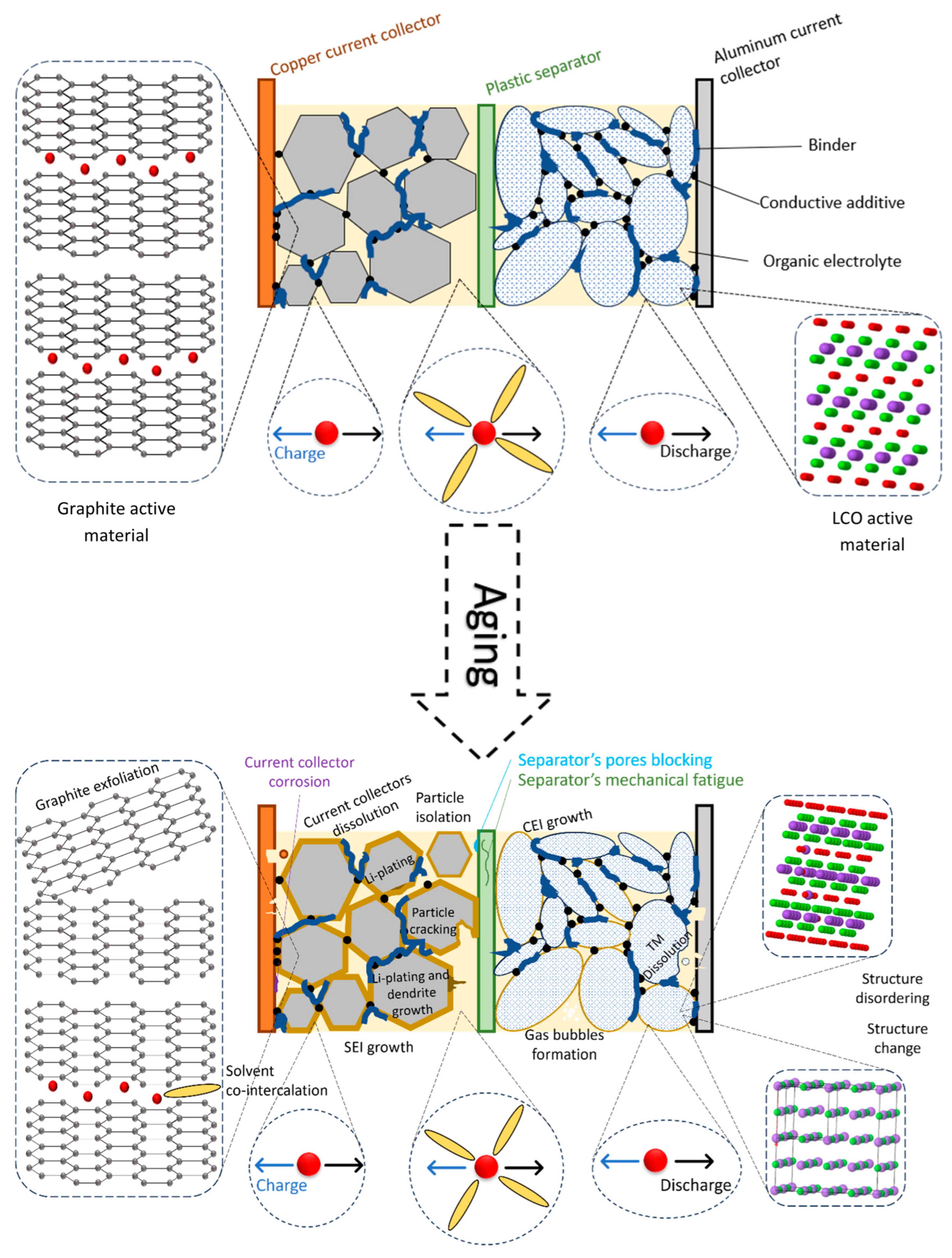
- SEI growth;
- lithium-plating;
- particle cracking due to mechanical stress (and the associated growth of the SEI on the cracks);
- loss of active material (LAM) due to mechanical stress and the internal cracks of the particles;
- oxidation of the electrolyte at the positive electrode.
2. State of the Art on Machine Learning Models to Predict Battery Aging Using Time Passed by the Cell between Thresholds
- The thresholds selected in previous studies were specific to the datasets used. In contrast, the present work proposes general thresholds applicable to any battery aging dataset, thus contributing to moving a step closer to a general battery aging model.
- Except for the study by Zhang et al. [42], which employed the NASA randomized battery dataset [44], the models available in the literature have not been applied to open-source databases where all cells do not experience the same ambient temperature during aging. Consequently, this paper presents the results from applying the method to two additional public datasets, wherein temperature thresholds are associated not only with cell heating but also with varying aging conditions, resulting in sparser data.
- This paper demonstrates the robustness of the method when applied to public datasets, thereby advancing the development of generalized battery aging models. These machine learning methods have not been previously applied to these datasets, and their usage introduces challenges that are distinct from those encountered before.
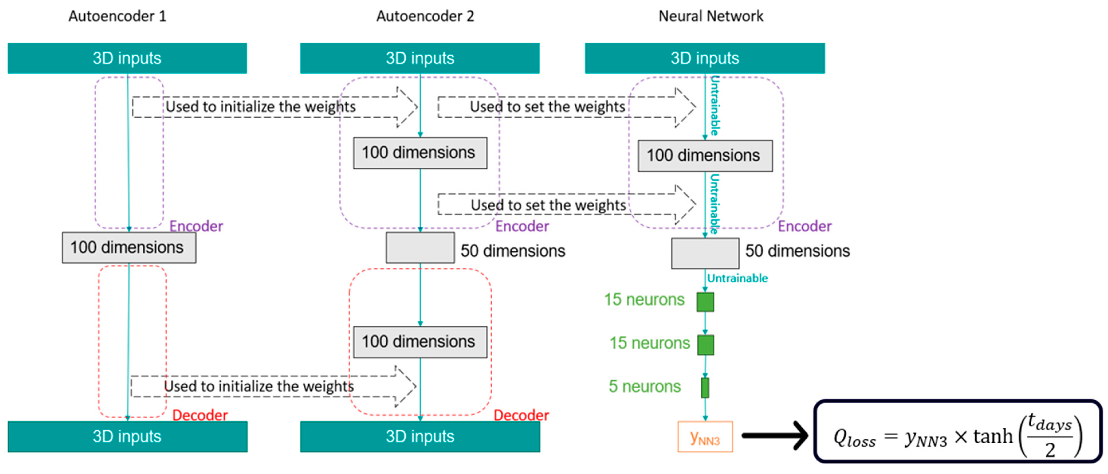
- Furthermore, to the best of the authors’ knowledge, this study is the first application of autoencoders for reducing the dimensionality of inputs based on the time spent.
- This study introduces novel inputs derived from zones that are not based on the time spent in a zone or the zone’s density. Instead, these novel inputs include the time integral of the current in the zone, that of the SOC, and that of the temperature. This approach enables the model to account for parameter variations within a zone.
3. Materials and Methods
3.1. Battery Aging Datasets Used
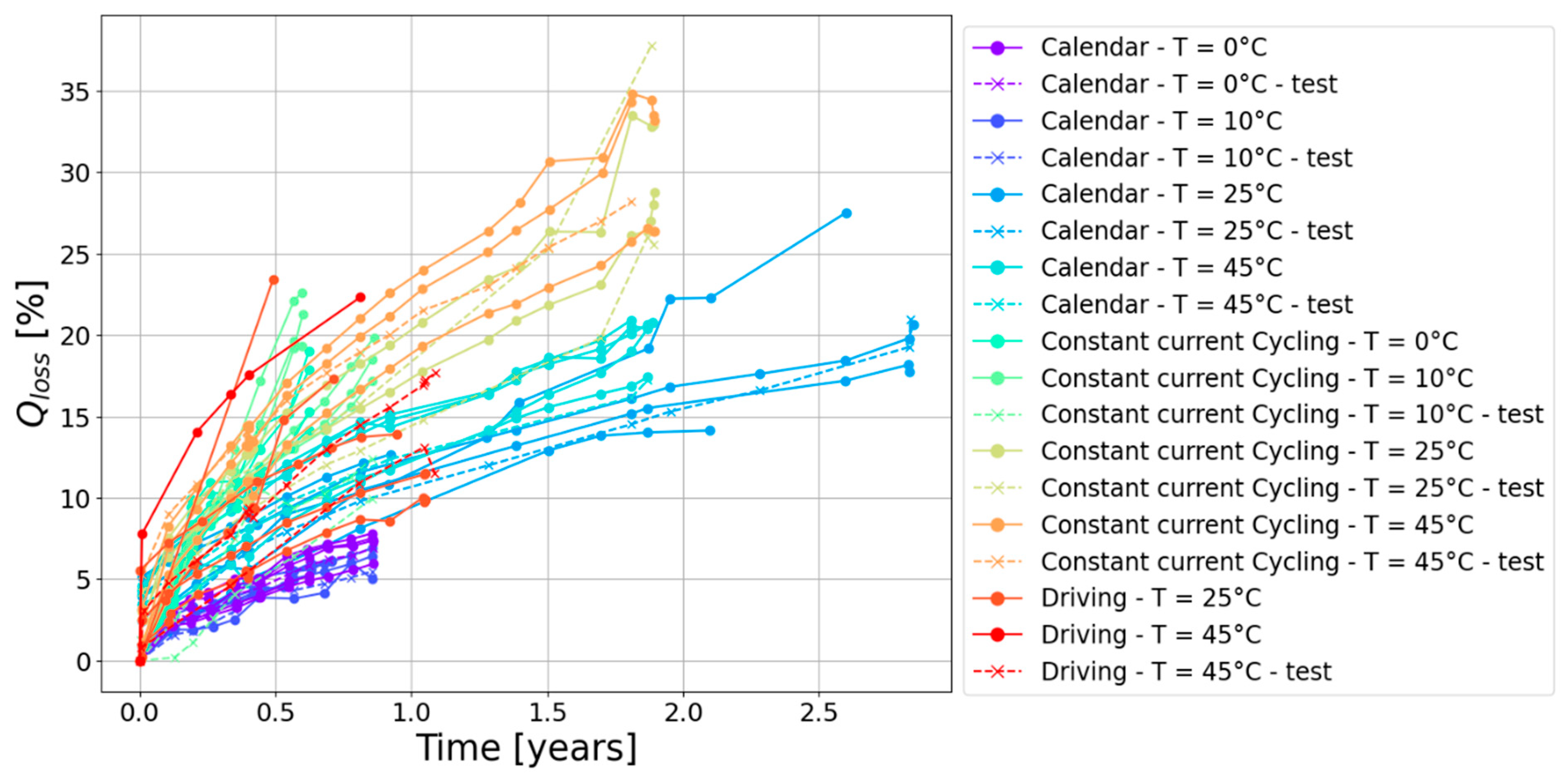
3.1.1. The EVERLASTING Dataset
- Cells 19 and 20 experienced CC cycle aging at 10 °C;
- Cell 34 underwent calendar aging at 10 °C and SOC = 90%;
- Cell 37 underwent calendar aging at 0 °C and SOC = 70%;
- Cell 63 experienced CC cycle aging at 45 °C;
- Cells 68 and 69 experienced driving aging at 45 °C between 70 and 90% SOC;
- Cell 72 underwent calendar aging at 45 °C and SOC = 10%;
- Cells 78 and 79 experienced CC cycle aging at 25 °C;
- Cell 96 underwent calendar aging at 25 °C and SOC = 90%.
3.1.2. The Bills Dataset
3.2. Empirical Models
- a basic aging model;
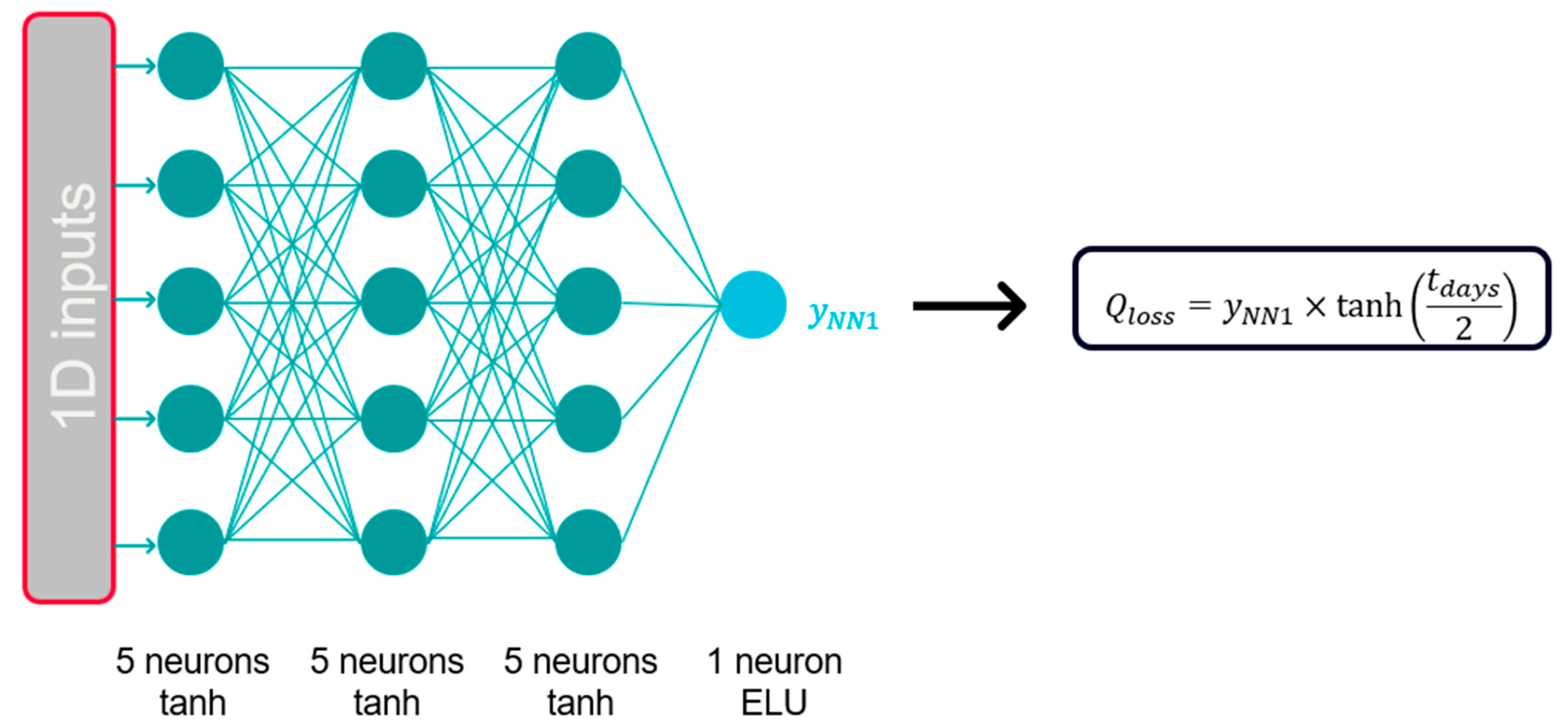
3.3. Machine Learning Models
- Age of the cell
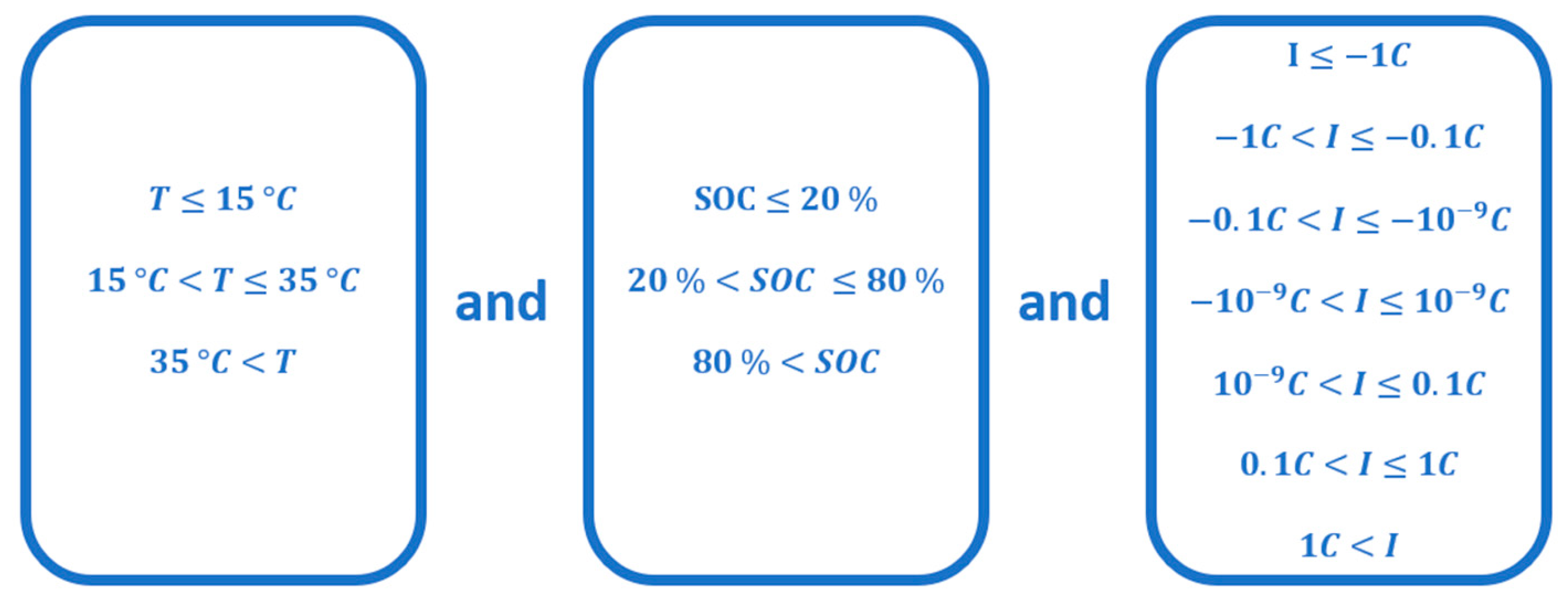
- Time spent by the cell with low SOC:
- Time spent by the cell with medium SOC:
- Time spent by the cell with high SOC:
- Time spent by the cell at a low temperature:
- Time spent by the cell at a medium temperature:
- Time spent by the cell at a high temperature:
- Time spent by the cell with a high discharge current:
- Time spent by the cell with a medium discharge current:
- Time spent by the cell with a low discharge current:
- Time spent by the cell almost in the calendar:
- Time spent by the cell with a low charge current:
- Time spent by the cell with a medium charge current:
- Time spent by the cell with a high charge current:
- where
- where
- where
- where
- where
4. Results and Discussion
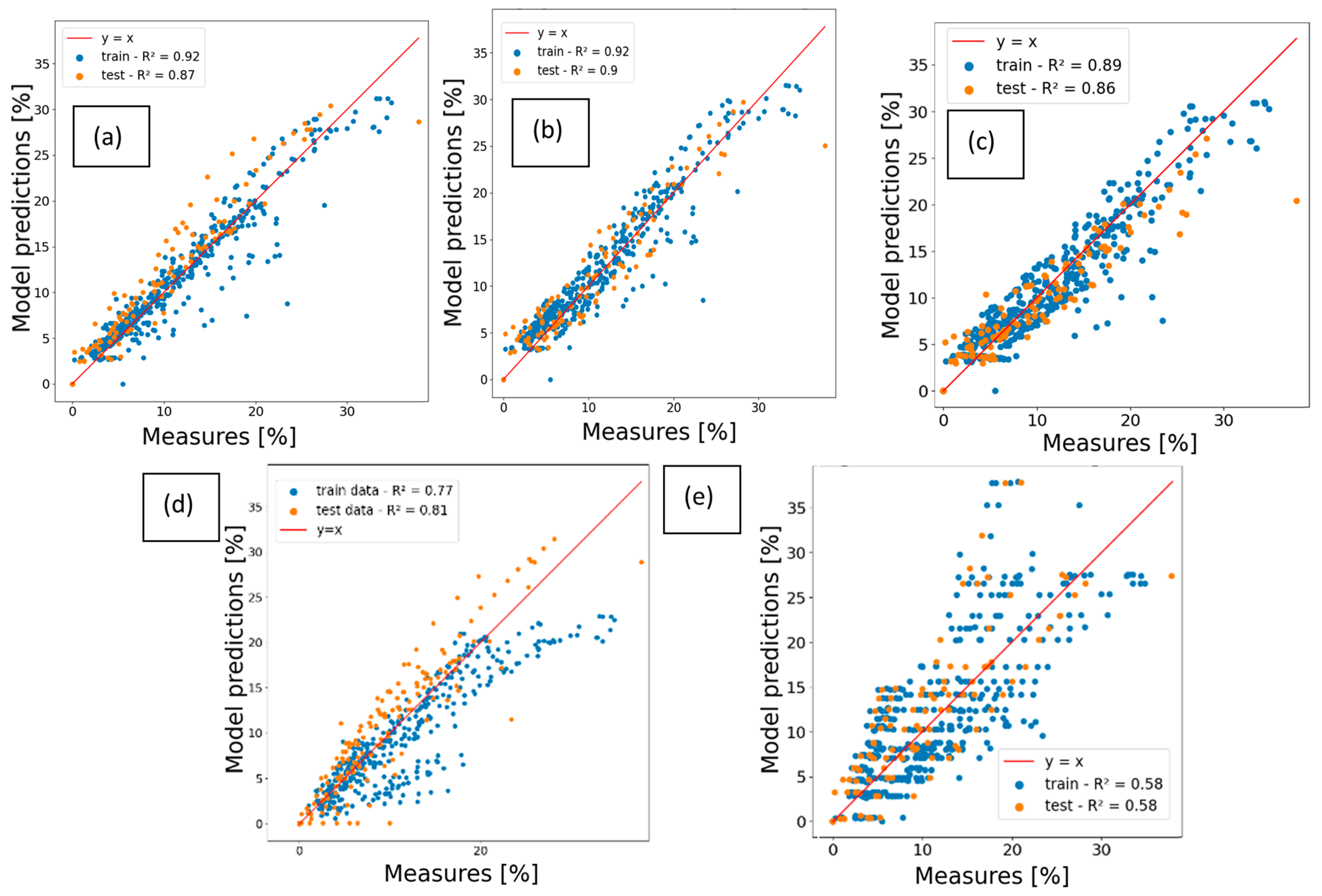
4.1. Aging Models on the EVERLASTING Dataset
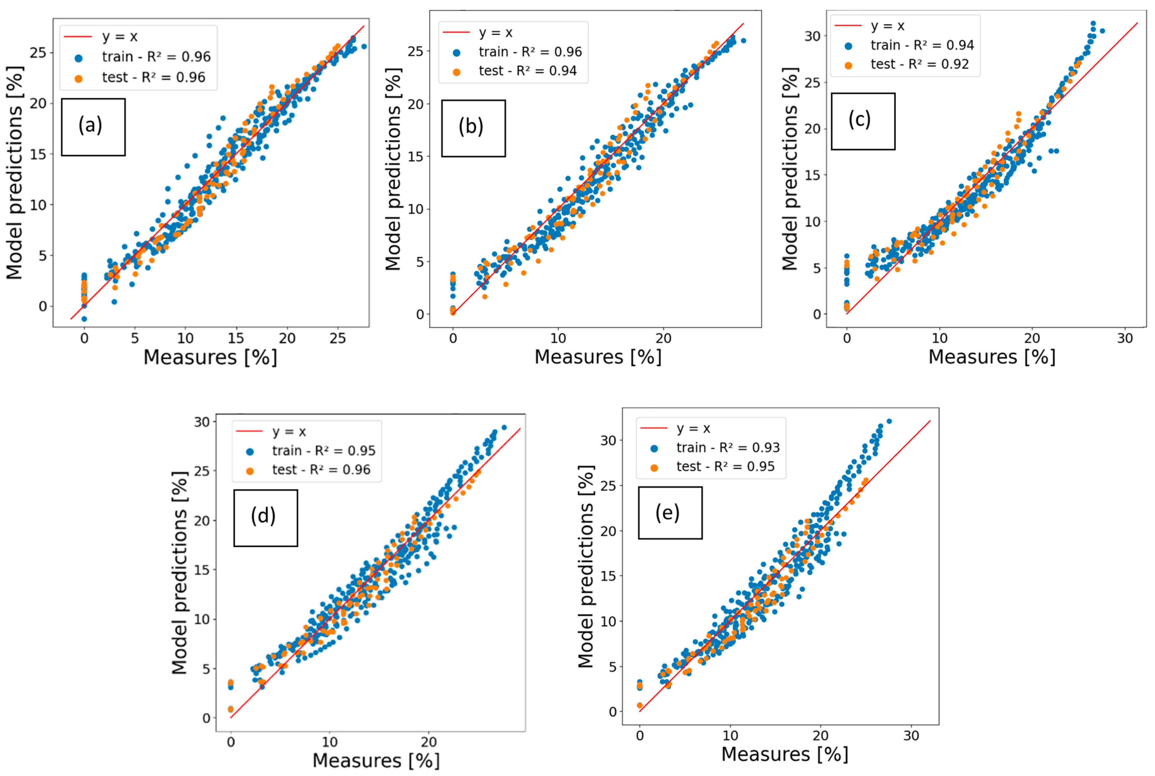
4.2. Aging Models on the Bills Dataset
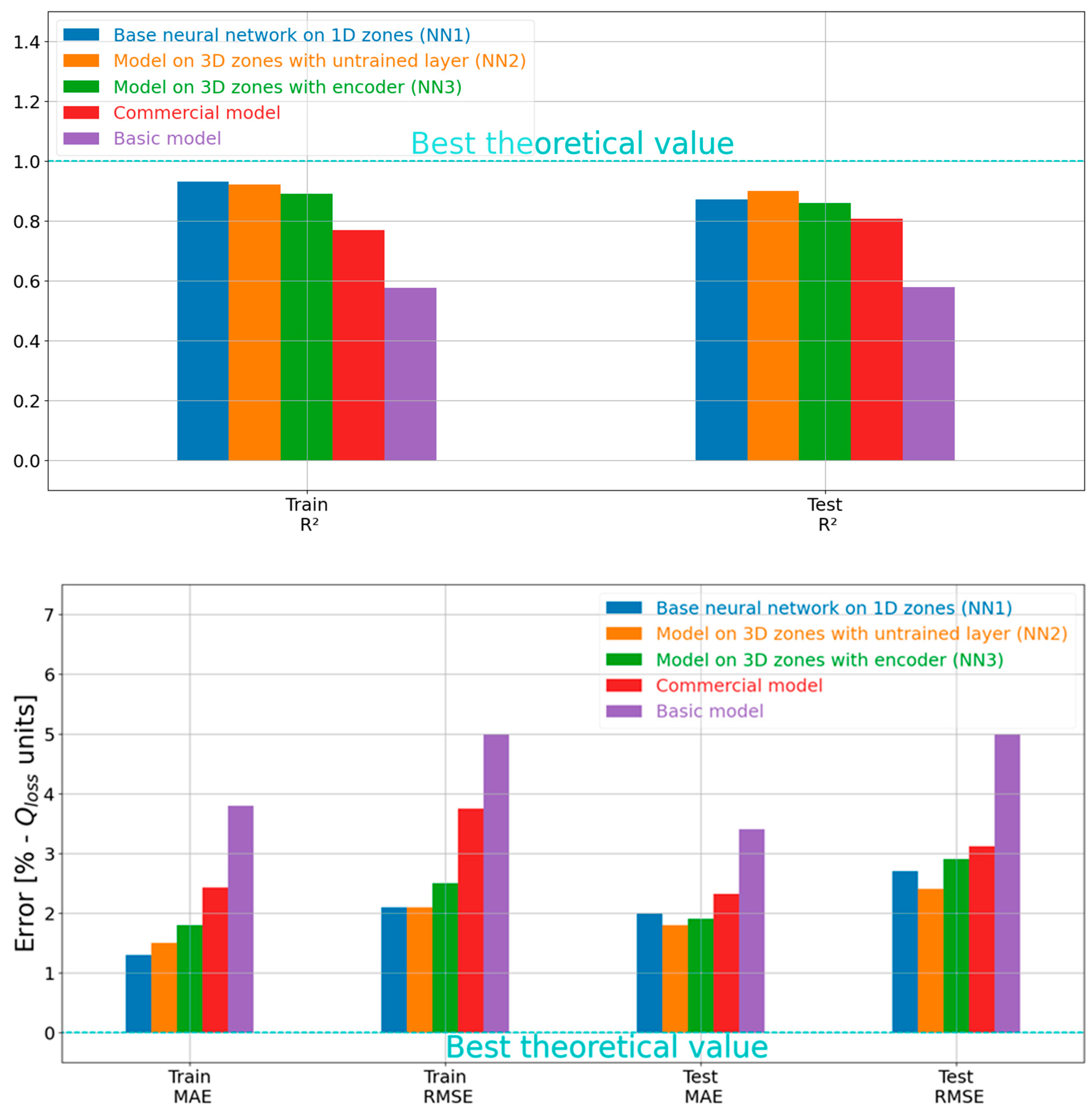
4.3. Overall Comparison of the Models
5. Conclusions
Author Contributions
Funding
Data Availability Statement
Conflicts of Interest
References
- Peng, J.; Meng, J.; Chen, D.; Liu, H.; Hao, S.; Sui, X.; Du, X. A Review of Lithium-Ion Battery Capacity Estimation Methods for Onboard Battery Management Systems: Recent Progress and Perspectives. Batteries 2022, 8, 229. [Google Scholar] [CrossRef]
- Mayemba, Q.; Mingant, R.; Li, A.; Ducret, G.; Venet, P. Aging datasets of commercial lithium-ion batteries: A review. J. Energy Storage 2024, 83, 110560. [Google Scholar] [CrossRef]
- University of Liverpool Lithium Cobalt Oxide–LiCoO2–Conduction Animation. Available online: https://www.chemtube3d.com/lib_lco-2/ (accessed on 10 April 2024).
- Maher, K.; Yazami, R. A study of lithium ion batteries cycle aging by thermodynamics techniques. J. Power Sources 2014, 247, 527–533. [Google Scholar] [CrossRef]
- McBrayer, J.D.; Rodrigues, M.-T.F.; Schulze, M.C.; Abraham, D.P.; Apblett, C.A.; Bloom, I.; Carroll, G.M.; Colclasure, A.M.; Fang, C.; Harrison, K.L.; et al. Calendar aging of silicon-containing batteries. Nat. Energy 2021, 6, 866–872. [Google Scholar] [CrossRef]
- Pelletier, S.; Jabali, O.; Laporte, G.; Veneroni, M. Battery degradation and behaviour for electric vehicles: Review and numerical analyses of several models. Transp. Res. Part B Methodol. 2017, 103, 158–187. [Google Scholar] [CrossRef]
- Fath, J.P.; Dragicevic, D.; Bittel, L.; Nuhic, A.; Sieg, J.; Hahn, S.; Alsheimer, L.; Spier, B.; Wetzel, T. Quantification of aging mechanisms and inhomogeneity in cycled lithium-ion cells by differential voltage analysis. J. Energy Storage 2019, 25, 100813. [Google Scholar] [CrossRef]
- Ahn, Y.; Jo, Y.N.; Cho, W.; Yu, J.-S.; Kim, K.J. Mechanism of Capacity Fading in the LiNi0.8Co0.1Mn0.1O2 Cathode Material for Lithium-Ion Batteries. Energies 2019, 12, 1638. [Google Scholar] [CrossRef]
- Chen, C.-F.; Barai, P.; Mukherjee, P.P. An overview of degradation phenomena modeling in lithium-ion battery electrodes. Curr. Opin. Chem. Eng. 2016, 13, 82–90. [Google Scholar] [CrossRef]
- Reniers, J.M.; Mulder, G.; Howey, D.A. Review and Performance Comparison of Mechanical-Chemical Degradation Models for Lithium-Ion Batteries. J. Electrochem. Soc. 2019, 166, A3189–A3200. [Google Scholar] [CrossRef]
- Rowden, B.; Garcia-Araez, N. A review of gas evolution in lithium ion batteries. Energy Rep. 2022, 6, 10–18. [Google Scholar] [CrossRef]
- Kabir, M.M.; Demirocak, D.E. Degradation mechanisms in Li-ion batteries: A state-of-the-art review. Int. J. Energy Res. 2017, 41, 1963–1986. [Google Scholar] [CrossRef]
- Gao, H.; Yan, Q.; Holoubek, J.; Yin, Y.; Bao, W.; Liu, H.; Baskin, A.; Li, M.; Cai, G.; Li, W.; et al. Enhanced Electrolyte Transport and Kinetics Mitigate Graphite Exfoliation and Li Plating in Fast-Charging Li-Ion Batteries. Adv. Energy Mater. 2023, 13, 2202906. [Google Scholar] [CrossRef]
- Winter, M.; Barnett, B.; Xu, K. Before Li Ion Batteries. Chem. Rev. 2018, 118, 11433–11456. [Google Scholar] [CrossRef] [PubMed]
- Zhang, Z.; Yang, J.; Huang, W.; Wang, H.; Zhou, W.; Li, Y.; Li, Y.; Xu, J.; Huang, W.; Chiu, W.; et al. Cathode-Electrolyte Interphase in Lithium Batteries Revealed by Cryogenic Electron Microscopy. Matter 2021, 4, 302–312. [Google Scholar] [CrossRef]
- Guo, L.; Thornton, D.B.; Koronfel, M.A.; Stephens, I.E.L.; Ryan, M.P. Degradation in lithium ion battery current collectors. J. Phys. Energy 2021, 3, 32015. [Google Scholar] [CrossRef]
- Vetter, J.; Novák, P.; Wagner, M.R.; Veit, C.; Möller, K.-C.; Besenhard, J.O.; Winter, M.; Wohlfahrt-Mehrens, M.; Vogler, C.; Hammouche, A. Ageing mechanisms in lithium-ion batteries. J. Power Sources 2005, 147, 269–281. [Google Scholar] [CrossRef]
- Chae, S.; Kim, N.; Ma, J.; Cho, J.; Ko, M. One-to-One Comparison of Graphite-Blended Negative Electrodes Using Silicon Nanolayer-Embedded Graphite versus Commercial Benchmarking Materials for High-Energy Lithium-Ion Batteries. Adv. Energy Mater. 2017, 7, 15. [Google Scholar] [CrossRef]
- Lin, C.; Tang, A.; Mu, H.; Wang, W.; Wang, C. Aging Mechanisms of Electrode Materials in Lithium-Ion Batteries for Electric Vehicles. J. Chem. 2015, 2015, 104673. [Google Scholar] [CrossRef]
- Yang, R.; Yu, G.; Wu, Z.; Lu, T.; Hu, T.; Liu, F.; Zhao, H. Aging of lithium-ion battery separators during battery cycling. J. Energy Storage 2023, 63, 107107. [Google Scholar] [CrossRef]
- Wheeler, W.; Venet, P.; Bultel, Y.; Sari, A.; Riviere, E. Aging in First and Second Life of G/LFP 18650 Cells: Diagnosis and Evolution of the State of Health of the Cell and the Negative Electrode under Cycling. Batteries 2024, 10, 137. [Google Scholar] [CrossRef]
- Abada, S.; Petit, M.; Lecocq, A.; Marlair, G.; Sauvant-Moynot, V.; Huet, F. Combined experimental and modeling approaches of the thermal runaway of fresh and aged lithium-ion batteries. J. Power Sources 2018, 399, 264–273. [Google Scholar] [CrossRef]
- O’Kane, S.E.J.; Ai, W.; Madabattula, G.; Alonso-Alvarez, D.; Timms, R.; Sulzer, V.; Edge, J.S.; Wu, B.; Offer, G.J.; Marinescu, M. Lithium-ion battery degradation: How to model it. Phys. Chem. Chem. Phys. 2022, 24, 7909–7922. [Google Scholar] [CrossRef]
- Lopetegi, I.; Plett, G.L.; Trimboli, M.S.; Yeregui, J.; Oca, L.; Rojas, C.; Miguel, E.; Iraola, U. Lithium-ion Battery Aging Prediction with Electrochemical Models: P2D vs. SPMe. In Proceedings of the 2023 IEEE Vehicle Power and Propulsion Conference (VPPC), Milan, Italy, 24–27 October 2023; IEEE: Piscataway, NJ, USA, 2023; pp. 1–7. [Google Scholar]
- Mingant, R.; Petit, M.; Belaïd, S.; Bernard, J. Data-driven model development to predict the aging of a Li-ion battery pack in electric vehicles representative conditions. J. Energy Storage 2021, 39, 102592. [Google Scholar] [CrossRef]
- Vermeer, W.; Chandra Mouli, G.R.; Bauer, P. A Comprehensive Review on the Characteristics and Modeling of Lithium-Ion Battery Aging. IEEE Trans. Transp. Electrif. 2022, 8, 2205–2232. [Google Scholar] [CrossRef]
- Bülow, F.; von Meisen, T. A review on methods for state of health forecasting of lithium-ion batteries applicable in real-world operational conditions. J. Energy Storage 2023, 57, 105978. [Google Scholar] [CrossRef]
- Sui, X.; He, S.; Vilsen, S.B.; Meng, J.; Teodorescu, R.; Stroe, D.-I. A review of non-probabilistic machine learning-based state of health estimation techniques for Lithium-ion battery. Appl. Energy 2021, 300, 117346. [Google Scholar] [CrossRef]
- Guo, W.; Sun, Z.; Vilsen, S.B.; Meng, J.; Stroe, D.I. Review of “grey box” lifetime modeling for lithium-ion battery: Combining physics and data-driven methods. J. Energy Storage 2022, 56, 105992. [Google Scholar] [CrossRef]
- Khaleghi, S.; Hosen, M.S.; van Mierlo, J.; Berecibar, M. Towards machine-learning driven prognostics and health management of Li-ion batteries. A comprehensive review. Renew. Sustain. Energy Rev. 2024, 192, 114224. [Google Scholar] [CrossRef]
- Cao, L.; Xu, R.; Bi, Y. Research on Life Prediction of Lithium-ion Battery based on WEMD-ARIMA Model. In Proceedings of the 2022 34th Chinese Control and Decision Conference (CCDC), Hefei, China, 15–17 August 2022; IEEE: Piscataway, NJ, USA, 2022; pp. 2774–2779. [Google Scholar]
- Jorge, I.; Mesbahi, T.; Samet, A.; Boné, R. Time Series Feature extraction for Lithium-Ion batteries State-Of-Health prediction. J. Energy Storage 2023, 59, 106436. [Google Scholar] [CrossRef]
- Lombardo, T.; Duquesnoy, M.; El-Bouysidy, H.; Årén, F.; Gallo-Bueno, A.; Jørgensen, P.B.; Bhowmik, A.; Demortière, A.; Ayerbe, E.; Alcaide, F.; et al. Artificial Intelligence Applied to Battery Research: Hype or Reality? Chem. Rev. 2022, 122, 10899–10969. [Google Scholar] [CrossRef]
- Nuhic, A.; Terzimehic, T.; Soczka-Guth, T.; Buchholz, M.; Dietmayer, K. Health diagnosis and remaining useful life prognostics of lithium-ion batteries using data-driven methods. J. Power Sources 2013, 239, 680–688. [Google Scholar] [CrossRef]
- You, G.; Park, S.; Oh, D. Real-time state-of-health estimation for electric vehicle batteries: A data-driven approach. Appl. Energy 2016, 176, 92–103. [Google Scholar] [CrossRef]
- Richardson, R.R.; Osborne, M.A.; Howey, D.A. Battery health prediction under generalized conditions using a Gaussian process transition model. J. Energy Storage 2019, 23, 320–328. [Google Scholar] [CrossRef]
- Song, L.; Zhang, K.; Liang, T.; Han, X.; Zhang, Y. Intelligent state of health estimation for lithium-ion battery pack based on big data analysis. J. Energy Storage 2020, 32, 101836. [Google Scholar] [CrossRef]
- Greenacre, M.; Groenen, P.J.F.; Hastie, T.; D’Enza, A.I.; Markos, A.; Tuzhilina, E. Principal component analysis. Nat. Rev. Methods Primers 2020, 2, 100. [Google Scholar] [CrossRef]
- Bülow, F.; von Mentz, J.; Meisen, T. State of health forecasting of Lithium-ion batteries applicable in real-world operational conditions. J. Energy Storage 2021, 44, 103439. [Google Scholar] [CrossRef]
- Severson, K.A.; Attia, P.M.; Jin, N.; Perkins, N.; Jiang, B.; Yang, Z.; Chen, M.H.; Aykol, M.; Herring, P.K.; Fraggedakis, D.; et al. Data-driven prediction of battery cycle life before capacity degradation. Nat. Energy 2019, 4, 383–391. [Google Scholar] [CrossRef]
- Yang, L.; Shami, A. On hyperparameter optimization of machine learning algorithms: Theory and practice. Neurocomputing 2020, 415, 295–316. [Google Scholar] [CrossRef]
- Zhang, Y.; Wik, T.; Bergström, J.; Pecht, M.; Zou, C. A machine learning-based framework for online prediction of battery ageing trajectory and lifetime using histogram data. J. Power Sources 2022, 526, 231110. [Google Scholar] [CrossRef]
- Attia, P.M.; Grover, A.; Jin, N.; Severson, K.A.; Markov, T.M.; Liao, Y.-H.; Chen, M.H.; Cheong, B.; Perkins, N.; Yang, Z.; et al. Closed-loop optimization of fast-charging protocols for batteries with machine learning. Nature 2020, 578, 397–402. [Google Scholar] [CrossRef]
- NASA. Available online: https://papers.phmsociety.org/index.php/phmconf/article/view/2490 (accessed on 3 April 2024).
- Greenbank, S.; Howey, D.A. Piecewise-linear modelling with automated feature selection for Li-ion battery end-of-life prognosis. Mech. Syst. Signal Process. 2023, 184, 109612. [Google Scholar] [CrossRef]
- Attia, P.M.; Bills, A.; Brosa Planella, F.; Dechent, P.; dos Reis, G.; Dubarry, M.; Gasper, P.; Gilchrist, R.; Greenbank, S.; Howey, D.; et al. Review—“Knees” in Lithium-Ion Battery Aging Trajectories. J. Electrochem. Soc. 2022, 169, 60517. [Google Scholar] [CrossRef]
- Trad, K.; Govindarajan, J. D2.3-Report Containing Aging Test Profiles and Test Results; EVERLASTING: Yakima, WA, USA, 2020; Available online: https://everlasting-project.eu/wp-content/uploads/2020/03/EVERLASTING_D2.3_final_20200228.pdf (accessed on 13 October 2024).
- Bills, A.; Viswanathan, V.; Sripad, S.; Frank, E.; Charles, D.; Fredericks, W.L. eVTOL Battery Dataset; Carnegie Mellon University: Pittsburgh, PA, USA, 2023. [Google Scholar]
- dos Reis, G.; Strange, C.; Yadav, M.; Li, S. Lithium-ion battery data and where to find it. Energy AI 2021, 5, 100081. [Google Scholar] [CrossRef]
- Hassini, M.; Redondo-Iglesias, E.; Venet, P. Lithium–Ion Battery Data: From Production to Prediction. Batteries 2023, 9, 385. [Google Scholar] [CrossRef]
- Yang, X.-G.; Liu, T.; Ge, S.; Rountree, E.; Wang, C.-Y. Challenges and key requirements of batteries for electric vertical takeoff and landing aircraft. Joule 2021, 5, 1644–1659. [Google Scholar] [CrossRef]
- CC BY. Available online: https://creativecommons.org/licenses/by/4.0/ (accessed on 13 October 2024).
- Siemens Digital Industries Software. Simcenter AMESim V2310 (Advanced Modeling Environment for Performing Simulations); Siemens Digital Industries Software: Plano, TX, USA, 2023. [Google Scholar]
- Jafari, M.; Khan, K.; Gauchia, L. Deterministic models of Li-ion battery aging: It is a matter of scale. J. Energy Storage 2018, 20, 67–77. [Google Scholar] [CrossRef]
- Huang, G.-B.; Zhu, Q.-Y.; Siew, C.-K. Extreme learning machine: Theory and applications. Neurocomputing 2006, 70, 489–501. [Google Scholar] [CrossRef]
- Wang, J.; Lu, S.; Wang, S.-H.; Zhang, Y.-D. A review on extreme learning machine. Multimed. Tools Appl. 2022, 81, 41611–41660. [Google Scholar] [CrossRef]
- Michelucci, U. An Introduction to Autoencoders. arXiv 2022, arXiv:2201.03898. [Google Scholar]
- Li, P.; Pei, Y.; Li, J. A comprehensive survey on design and application of autoencoder in deep learning. Appl. Soft Comput. 2023, 138, 110176. [Google Scholar] [CrossRef]


| Number | Phenomenon | Reference |
|---|---|---|
| 1 | Solid Electrolyte Interphase (SEI) growth, which can be considered the most important degradation phenomenon (the composition and behavior are different in silicon-containing negative electrodes) | [4,5] |
| 2 | Lithium plating and dendrite growth | [6,7] |
| 3 | Particle cracking, which is due to the volume changes during lithiation | [7,8,9] |
| 4 | Gas bubbles formation and electrolyte drying (mainly the formation of H2, due to the decomposition of the organic molecules in the electrolyte) | [7,10,11] |
| 5 | Structure changes in the active material happen when the crystal structure of the active material changes and lithium cannot be inserted any more | [12] |
| 6 | Transition metals dissolution (the transition metals concerned are mainly Ni, Co, and Mn, dissolving into the electrolyte) | [8] |
| 7 | Graphite exfoliation and solvent co-intercalation, happens when the electrolyte solvent inserts itself into the graphite with the lithium-ion and separates the graphite sheets | [13,14] |
| 8 | The growth of the positive electrode–electrolyte interface | [15] |
| 9 | The corrosion or dissolution of the current collectors | [16] |
| 10 | The loss of electric contact | [12,17,18] |
| 11 | The decomposition of the binders | [19] |
| 12 | The decomposition of the electrolyte | [12] |
| 13 | The degradation of the separator | [20] |
| Study | Dataset | Open-Source Data? | Method to Fix Thresholds | Inputs | Outputs | Model | Temperature |
|---|---|---|---|---|---|---|---|
| Nuhic 2013 [34] | 5 batteries, no reference to another work or the data publication | No | Not shared | 2D inputs (I&T and SOC&T) and rainflow counting of the SOC | SVR | Yes | |
| You 2016 [35] | Private | No | K-Means clustering | Density of the 3D zones of (I, T, SOC) | SOH | SVM, ANN | Yes |
| Richardson 2019 [36] | NASA Randomized Battery Dataset | Yes | Arbitrary (Proposed 1D data but did not implement it) | Ah-throughput, , and time. | GPR | Proposed to consider it but did not implement | |
| Song 2020 [37] | BHEV and BEV data from real vehicles | No | Arbitrary | Principal components of the mileage and the 1D distribution of current, SOC, and temperature | Q | ANN | Yes |
| von Bülow 2021 [39] | Severson [40] | Yes | Arbitrary | 2D, 3D | ANN and GPR | Yes | |
| Zhang 2022 [42] | Severson [40] Attia [43], NASA randomized battery dataset [44], and a dataset based on actual measurements from plug-in hybrid electric vehicles (PHEV). | Partly | Not shared | Derived from the histogram data | Random forest regressions, support vector regressions, ANN, and GPR | Yes | |
| Greenbank 2023 [45] | Severson [40] Attia [43] | Yes | Based on the distribution | Time spent (1D) | Qloss t+12 h | Piecewise linear model, Gaussian process regression | Yes |
| Present work | EVERLASTING [47] Bills [48] | Yes | Arbitrary | Time spent (1D) and time integrals (3D) | ANN, ELM, auto-encoders | Yes |
| Temperature | I Profile 70–90% SOC | I Profile 10–90% SOC | P Profile 10–90% SOC |
|---|---|---|---|
| 0 °C | 2 | 2 | |
| 10 °C | 2 | 2 | |
| 25 °C | 2 | 2 | 2 |
| 45 °C | 2 | 2 |
| Temperature | Charge C-Rate | Discharge C-Rate | Number of Cells |
|---|---|---|---|
| 0 °C | 0.5 | 1.5 | 2 |
| 0 °C | 1 | 1.5 | 2 |
| 10 °C | 0.5 | 1.5 | 2 |
| 10 °C | 0.5 | 0.5 | 2 |
| 10 °C | 0.5 | 3 | 2 |
| 10 °C | 1 | 1.5 | 2 |
| 25 °C | 0.5 | 1.5 | 2 |
| 25 °C | 0.5 | 0.5 | 2 |
| 25 °C | 0.5 | 3 | 2 |
| 25 °C | 1 | 1.5 | 2 |
| 45 °C | 0.5 | 1.5 | 2 |
| 45 °C | 0.5 | 0.5 | 2 |
| 45 °C | 0.5 | 3 (a) | 2 |
| 45 °C | 1 | 1.5 | 2 |
| SOC Temperature | 10% | 70% | 90% |
|---|---|---|---|
| 0 °C | 2 | 2 | 2 |
| 10 °C | 2 | 2 | 2 |
| 25 °C | 2 | 2 | 2 |
| 45 °C | 2 | 2 | 2 |
| Phase | Definition | End Criteria |
|---|---|---|
| Take-off | P = 54 W | t = 75 s |
| Cruise | P = 16 W | t = 800 s |
| Landing | P = 54 W | t = 105 s |
| Rest 1 | I = 0 A | T < 27 °C |
| CC Charge | I = 1 C | U > 4.2 V |
| CV Charge | U = 4.2 V | I < C/30 |
| Rest 2 | I = 0 A | T < 35 °C |
| Mission Profile | Cells Impacted | Number of Data Points |
|---|---|---|
| Baseline | VAH01, VAH17, VAH27 | 52 |
| Short cruise (400 s) | VAH12 | 47 |
| Short cruise (600 s) | VAH13, VAH26 | 45 |
| Extended cruise (1000 s) | VAH02, VAH15, VAH22 | 36 |
| 10% power reduction during discharge | VAH05, VAH28 | 30 and 24 |
| 20% power reduction during discharge | VAH11 | 44 |
| CC charge current reduced to C/2 | VAH06, VAH24 | 37 |
| CC charge current brought up to 1.5 C | VAH16, VAH20 | 24 |
| CV charge voltage reduced to 4.0 V | VAH07 | 6 |
| CV charge voltage reduced to 4.1 V | VAH23 | 15 |
| Thermal chamber temperature reduced to 20 °C | VAH09, VAH25 | 35 |
| Thermal chamber temperature brought up to 30 °C | VAH10 | 29 |
| Thermal chamber temperature brought up to 35 °C | VAH30 | 19 |
Disclaimer/Publisher’s Note: The statements, opinions and data contained in all publications are solely those of the individual author(s) and contributor(s) and not of MDPI and/or the editor(s). MDPI and/or the editor(s) disclaim responsibility for any injury to people or property resulting from any ideas, methods, instructions or products referred to in the content. |
© 2024 by the authors. Licensee MDPI, Basel, Switzerland. This article is an open access article distributed under the terms and conditions of the Creative Commons Attribution (CC BY) license (https://creativecommons.org/licenses/by/4.0/).
Share and Cite
Mayemba, Q.; Ducret, G.; Li, A.; Mingant, R.; Venet, P. General Machine Learning Approaches for Lithium-Ion Battery Capacity Fade Compared to Empirical Models. Batteries 2024, 10, 367. https://doi.org/10.3390/batteries10100367
Mayemba Q, Ducret G, Li A, Mingant R, Venet P. General Machine Learning Approaches for Lithium-Ion Battery Capacity Fade Compared to Empirical Models. Batteries. 2024; 10(10):367. https://doi.org/10.3390/batteries10100367
Chicago/Turabian StyleMayemba, Quentin, Gabriel Ducret, An Li, Rémy Mingant, and Pascal Venet. 2024. "General Machine Learning Approaches for Lithium-Ion Battery Capacity Fade Compared to Empirical Models" Batteries 10, no. 10: 367. https://doi.org/10.3390/batteries10100367
APA StyleMayemba, Q., Ducret, G., Li, A., Mingant, R., & Venet, P. (2024). General Machine Learning Approaches for Lithium-Ion Battery Capacity Fade Compared to Empirical Models. Batteries, 10(10), 367. https://doi.org/10.3390/batteries10100367