A Comprehensive Flow–Mass–Thermal–Electrochemical Coupling Model for a VRFB Stack and Its Application in a Stack Temperature Control Strategy

Abstract

In this work, a comprehensive multi-physics electrochemical hybrid stack model is developed for a vanadium redox flow battery (VRFB) stack considering electrolyte flow, mass transport, electrochemical reactions, shunt currents, and as heat generation and transfer simultaneously. Compared with other VRFB stack models, this model is more comprehensive in considering the influence of multiple factors. Based on the established model, the electrolyte flow rate distribution across cells in the stack is investigated. The distribution and variation in shunt currents, single-cell current and single-cell voltage are analyzed. The distribution and variation in temperature and heat generation and heat transfer are also researched. It can be found that the VRFB stack temperature will exceed 40 °C when operating at 60 A and 100 mA cm⁻² at an ambient temperature of 30 °C, which will lead to electrolyte ion precipitation, affecting the performance and safety of the battery. To control the stack temperature below 40 °C, a new tank cooling control strategy is proposed, and the suitable starting cooling point and the controlled temperature are specified. Compared with the common room cooling strategy, the new tank cooling strategy reduces energy consumption by 27.18% during 20 charge–discharge cycles.

1. Introduction

Traditional primary energy sources not only lead to environmental pollution and emit vast amounts of carbon, but they are also unable meet the increasing energy demand of human society. Renewable energies are able to solve the problem due to their environmentally friendly and sustainable features [1]. However, due to discontinuous and unstable characteristics, renewable energy cannot be effectively utilized. The combined utilization of energy storage systems and renewable energy is needed. As a kind of energy storage system, the vanadium redox flow battery (VRFB) stands out due to its individual control of power and capacity, good safety, outstanding cyclic performance and easy capacity restoration [2].

The VRFB system consists of a stack, circulating pumps and two electrolyte storage tanks, wherein the stack is constructed by superimposing several single cells in series alignment. The electrolyte is transported to the cell through the pipe, manifold and channel, and the reversible redox reaction occurs in cells to realize the conversion of chemical energy and electric energy; in the process, heat is generated or absorbed. The generating and absorbing heat result in temperature variations of the VRFB during long charge–discharge cycles [3]. Studies have shown that vanadium ions can be stable in the temperature range from 5 to 40 °C. VO₂⁺ ions will precipitate when the temperature is higher than 40 °C, and V²⁺ and V³⁺ will precipitate when the temperature is lower than 5 °C [4]. Obviously, an unsuitable temperature will lead to blockage in the electrode and membrane, and may even result in battery operation failure [5]. Moreover, the electrolyte flow rate varies with different cells due to the parallel arrangement of different single cells in the stack. A low flow rate in certain cells gives rise to weak mass transport and high overpotential, which are detrimental to the performance of a VRFB stack [2]. For the reason that the electrolyte flowing in the flow frame is conductive, the shunt currents exist in the manifolds and channels [6]. The shunt currents result in a lower effective current in the porous electrode during the charging process and increase the charging time. Meanwhile, the effective current in the porous electrode is higher than the applied current during the discharging process due to the shunt currents, which increase the overpotential and decrease the performance [7].

It can be discovered that the performance of a VRFB stack is closely related with temperature, electrolyte flow and mass transport in cell and shunt currents in manifolds and channels. Many multi-physics models have been built by researchers to investigate the temperature, electrolyte flow, mass transport and shunt currents inside a VRFB stack. AL-Fetlawi et al. [8] established a transient 2D non-isothermal model to explore the electrolyte temperature distribution in a cell of a VRFB. However, the non-isothermal model neglects the heat transfer between the cell and external air. The study found that the difference in the electrolyte temperature in a cell is slight due to the forced convection of the electrolyte in the cell. Tang et al. [9,10] proposed a thermodynamic model for a VRFB stack, taking mass balance and energy conservation into account to explore the influence of the self-discharge reaction on the VRFB temperature. However, the thermodynamic model ignores the non-uniform distribution of temperature and electrolyte flow in the stack and the shunt currents are also neglected. They found that the self-discharge reaction has an obvious effect on the increased temperature of the electrolyte when the battery is on standby, but the heat generation of the self-discharge reaction can be ignored in the charge–discharge process, and the heat generation of the cell resistance has a significant influence on the total heat generation. Wei et al. [11] developed a VRFB stack dynamic thermo-hydraulic model considering the flow and temperature differences between cells to explore the influence of flow patterns on the stack temperature, which however excluded the influence of shunt currents. The study found that different stack flow patterns have an obvious influence on the flow distribution and temperature of the stack, and the serpentine–parallel pattern effectively controls the electrolyte temperature of the stack. Ren et al. [3] established an electrochemical–thermal coupling model considering all heat sources and heat transfer paths as well as shunt currents inside the VRFB stack to investigate the heat generation rates from different paths during charge–discharge processes. However, the electrochemical–thermal coupling model assumed the uniform distribution of electrolyte flow and temperature across different cells. The results showed that the heat generation of the electrochemical reversible reaction and the overpotential are dominant in the total heat. Trovò et al. [12] built a VRFB stack dynamic thermal model accounting for temperature distribution across different cells and shunt currents to explore the variation in temperature in the stack. However, this model did not consider the non-uniform distribution of the electrolyte flow rate across different cells. In summary, scholars used the lumped model to study the thermal behavior of a VRFB on the stack scale. The lumped model simplifies the thermal model to a zero-dimensional model, which considers the cell, pipe and tank to be simplified to a single point. The complete lumped model includes mass balance, electrochemistry and energy balance equations, in addition to the equivalent circuit model and electrolyte flow resistance model coupled in it. The mass balance equation takes into account the flow of the electrolyte between the cell and the tank, the effect of charging and discharging currents, and the transmembrane penetration of ions, which is used to calculate the ion concentration in the cell and the tank. The electrochemical equation simultaneously considers ohmic polarization, active polarization and concentration polarization; the voltage of each cell is obtained by calculating the open-circuit voltage and overpotential. The equivalent circuit model calculates the current of each cell by calculating the current flowing into the channel and manifold through Kirchhoff’s law. Referring to the equivalent circuit model, the electrolyte resistance model is established, which calculates the electrolyte flow resistance by using Kirchhoff’s law to obtain the electrolyte flow rate of each cell. The energy balance equation calculates the temperature change of the cell by calculating heat generation and absorption, as well as the heat transfer between the VRFB system and the environment during charging and discharging. Up to now, established models either ignore the non-uniform distribution across different cells or neglect shunt currents in a VRFB stack. It is essential to establish a multi-physics VRFB model considering the non-uniform distribution of temperature, electrolyte flow and mass transport and containing shunt currents in manifolds and channels.

In addition, researchers revealed that the maximum temperature in a VRFB stack will be higher than 50 °C after long operation periods, especially at high currents [12]. Therefore, it is necessary to carry out cooling control of the VRFB. Wei et al. [11] developed a shell and tube heat exchanger to control the cooling of the electrolyte temperature inside a VRFB stack and reduced the temperature of the electrolyte by 7 °C. Wang et al. [7] proposed a room cooling strategy using air conditioning to reduce the temperature of a VRFB stack and the energy consumption. They found that the proposed strategy saved 48% of the energy consumption of air conditioning. Nowadays, the most commonly used methods of cooling control for commercial VRFB systems are gas cooling of the battery through air conditioning [13]. Nevertheless, so far, only a few studies have implemented cooling control strategies using air conditioning for a VRFB stack. More effective cooling control strategies need to be proposed.

In this work, a multi-physics VRFB stack model considering the non-uniform distribution of temperature, electrolyte flow, mass transfer and shunt currents in manifolds and channels is established. The model takes into account the influence of many factors on the temperature of the cell and can predict the temperature change of the cell more accurately. In addition, compared with multidimensional models, the lumped model can save a lot of computing resources. The model is built on mass balance, electrochemistry and energy balance equations, and combines the electrolyte flow network model for calculating flow rates and the equivalent circuit model for calculating shunt currents. The distribution of temperature, electrolyte flow and electrical parameters across different cells is researched. Moreover, the multi-physical VRFB stack model is used to calculate the cell temperature, and the middle cell temperature is calculated to be the highest, so it is used to refer to the stack temperature. Cooling control is carried out through an air conditioner, and the temperature of the middle cell is adjusted below 40 °C to avoid electrolyte precipitation and stack blockage. In order to reduce the energy consumption of air conditioning, a new tank cooling control strategy is proposed.

2. VRFB Multi-Physics Stack Model

In this study, a multi-physics VRFB stack model is established by using Matlab/Simulink R2022b, which contains the mass balance equation, electrolyte flow network model, equivalent circuit model, electrochemical reaction equation and energy balance equation to more accurately predict the distribution and variation in key physical quantities across the cells in the stack. The following assumptions have been adopted:

• Due to forced convection, the temperature and concentration of the electrolyte are uniformly distributed within a cell and a tank [14].
• In the charge–discharge process, oxygen and hydrogen evolution reactions do not occur [14].
• The self-discharge reactions on both sides of the membrane are instantaneous [12].
• The conductivities of various components are constant [12].
• The electrolyte volume remains constant [12].
• The kinetic constants and diffusion coefficients are temperature-independent [3,15].
• Sulfuric acid is fully ionized [2].

In the charge–discharge process, electrochemical reactions take place on positive and negative electrodes.

Positive side:

$$\mathrm{V}{\mathrm{O}}^{2+}+{\mathrm{H}}_2\mathrm{O}\rightleftharpoons \mathrm{V}{\mathrm{O}}_2^{+}+2{\mathrm{H}}^{+}+{\mathrm{e}}^{-}, E_0^{+}=1.0 \mathrm{V}$$

(1)

Negative side:

$${\mathrm{V}}^{3+}+{\mathrm{e}}^{-}\rightleftharpoons {\mathrm{V}}^{2+}, E_0^{-}=-0.26 \mathrm{V}$$

(2)

Here, $E_0^{+}$ and $E_0^{-}$ are the standard potential of the positive and negative electrode reactions.

Although the cathode and anode electrolyte are separated through the membrane, due to the permeability of membrane, the vanadium ions transfer across the membrane and the self-discharge reactions take place. When a small quantity of V²⁺ and V³⁺ ions in the negative side transport to the positive side across the membrane, V²⁺ and V³⁺ ions will be oxidized by excessive VO₂⁺ ions. The self-discharge reactions of the positive side area as follows [16]:

$${\mathrm{V}}^{2+}+2\mathrm{V}{\mathrm{O}}_2^{+}+2{\mathrm{H}}^{+}\to 3\mathrm{V}{\mathrm{O}}^{2+}+{\mathrm{H}}_2\mathrm{O}$$

(3)

$${\mathrm{V}}^{3+}+\mathrm{V}{\mathrm{O}}_2^{+}\to 2\mathrm{V}{\mathrm{O}}^{2+}$$

(4)

Similarly, the VO₂⁺ and VO²⁺ ions in the positive side transport across the membrane to the negative side and are reduced by excessive V²⁺ ions. The self-discharge reactions of the negative side are as follows:

$$\mathrm{V}{\mathrm{O}}^{2+}+{\mathrm{V}}^{2+}+2{\mathrm{H}}^{+}\to 2{\mathrm{V}}^{3+}+{\mathrm{H}}_2\mathrm{O}$$

(5)

$$\mathrm{V}{\mathrm{O}}_2^{+}+2{\mathrm{V}}^{2+}+4{\mathrm{H}}^{+}\to 3{\mathrm{V}}^{3+}+2{\mathrm{H}}_2\mathrm{O}$$

(6)

2.1. Mass Balance

For a single cell in the stack, the mass variation derives from the electrolyte flow between the cell and tank, the electrochemical reactions, transmembrane diffusion and the self-discharge reactions in both sides of the cell. The concentrations of vanadium ions in the n-th cell can be determined through the application of mass balance equations, wherein the current is positive during the charging process and negative during the discharging process [17]:

$$V_e{\displaystyle \frac{d{c}_{2,n}}{dt}}=Q_n(c_{2,\mathrm{tank}}-c_{2,n})+{\displaystyle \frac{I_n}{zF}}-k_2{\displaystyle \frac{c_{2,n}}{d}}S-k_4{\displaystyle \frac{c_{4,n}}{d}}S-2k_5{\displaystyle \frac{c_{5,n}}{d}}S$$

(7)

$$V_e{\displaystyle \frac{d{c}_{3,n}}{dt}}=Q_n(c_{3,\mathrm{tank}}-c_{3,n})-{\displaystyle \frac{I_n}{zF}}-k_3{\displaystyle \frac{c_{3,n}}{d}}S+2k_4{\displaystyle \frac{c_{4,n}}{d}}S+3k_5{\displaystyle \frac{c_{5,n}}{d}}S$$

(8)

$$V_e{\displaystyle \frac{d{c}_{4,n}}{dt}}=Q_n\left(c_{4,\mathrm{tank}}-c_{4,n}\right)-{\displaystyle \frac{I_n}{zF}}-k_4{\displaystyle \frac{c_{4,n}}{d}}S+3k_2{\displaystyle \frac{c_{2,n}}{d}}S+2k_3{\displaystyle \frac{c_{3,n}}{d}}S$$

(9)

$$V_e{\displaystyle \frac{d{c}_{5,n}}{dt}}=Q_n(c_{5,\mathrm{tank}}-c_{5,n})+{\displaystyle \frac{I_n}{zF}}-k_5{\displaystyle \frac{c_{5,n}}{d}}S-2k_2{\displaystyle \frac{c_{2,n}}{d}}S-k_3{\displaystyle \frac{c_{3,n}}{d}}S$$

(10)

where $V_e$ is the volume of the electrode, $I_n$ and $Q_n$ are the current and flow rate of the n-th cell, respectively, $c_{i,n}$ and $c_{i,\mathrm{tank}}$ represent the concentration of vanadium ions in the cell and tank, respectively, $z$ is the number of electrons in the electrochemistry reaction, $F$ is the Faraday’s constant, $S$ and $d$ are the area and thickness of the membrane, as shown in

Table 1. The dimensions of the components in this model.

Symbol	Parameter	Value
We × He × Le	Electrode dimension	30 cm × 20 cm × 0.4 cm [12]
d	Membrane thickness	5 × 10−5 m [12]
Ama × Lma	Manifold dimension	7.065 cm2 × 2 cm [18,19]
Hch × Wch × Lch	Channel dimension	4 mm × 10 mm × 50 mm [2,19]
Api × Lpi	Pipe dimension	7.065 cm2 × 2 m [18,20]
Atank × Htank	Tank dimension	0.24 m2 × 1 m [10]

, and $k_i$ is the transmembrane diffusion coefficient of vanadium ions.

For the electrolyte storage tanks, the mass variation derives from the electrolyte flow between the stack and tank. The concentration can be calculated by using the following equations based on mass conservation:

$$V_{\mathrm{tank}}{\displaystyle \frac{d{c}_{2,\mathrm{tank}}}{dt}}=\sum _{n=1}^N{Q}_n(c_{2,n}-c_{2,\mathrm{tank}})$$

(11)

$$V_{\mathrm{tank}}{\displaystyle \frac{d{c}_{3,\mathrm{tank}}}{dt}}=\sum _{n=1}^N{Q}_n(c_{3,n}-c_{3,\mathrm{tank}})$$

(12)

$$V_{\mathrm{tank}}{\displaystyle \frac{d{c}_{4,\mathrm{tank}}}{dt}}=\sum _{n=1}^N{Q}_n(c_{4,n}-c_{4,\mathrm{tank}})$$

(13)

$$V_{\mathrm{tank}}{\displaystyle \frac{d{c}_{5,\mathrm{tank}}}{dt}}=\sum _{n=1}^N{Q}_n(c_{5,n}-c_{5,\mathrm{tank}})$$

(14)

where $V_{\mathrm{tank}}$ is the electrolyte volume in the tank.

The concentration of hydrogen ions in the positive and negative electrodes is calculated by using the following formula [2]:

$$\begin{gathered} c_{{\mathrm{H}}^{+}}^{+}=c_{{\mathrm{H}}^{+},0}^{+}-c\cdot \mathrm{SOC} \\ {c}_{{\mathrm{H}}^{+}}^{-}=c_{{\mathrm{H}}^{+},0}^{-}-c\cdot (1-\mathrm{SOC}) \end{gathered}$$

(15)

where $c_{{\mathrm{H}}^{+},0}^{+}$ and $c_{{\mathrm{H}}^{+},0}^{-}$ are the initial concentrations of H⁺ and $c$ is the total concentration of vanadium ions.

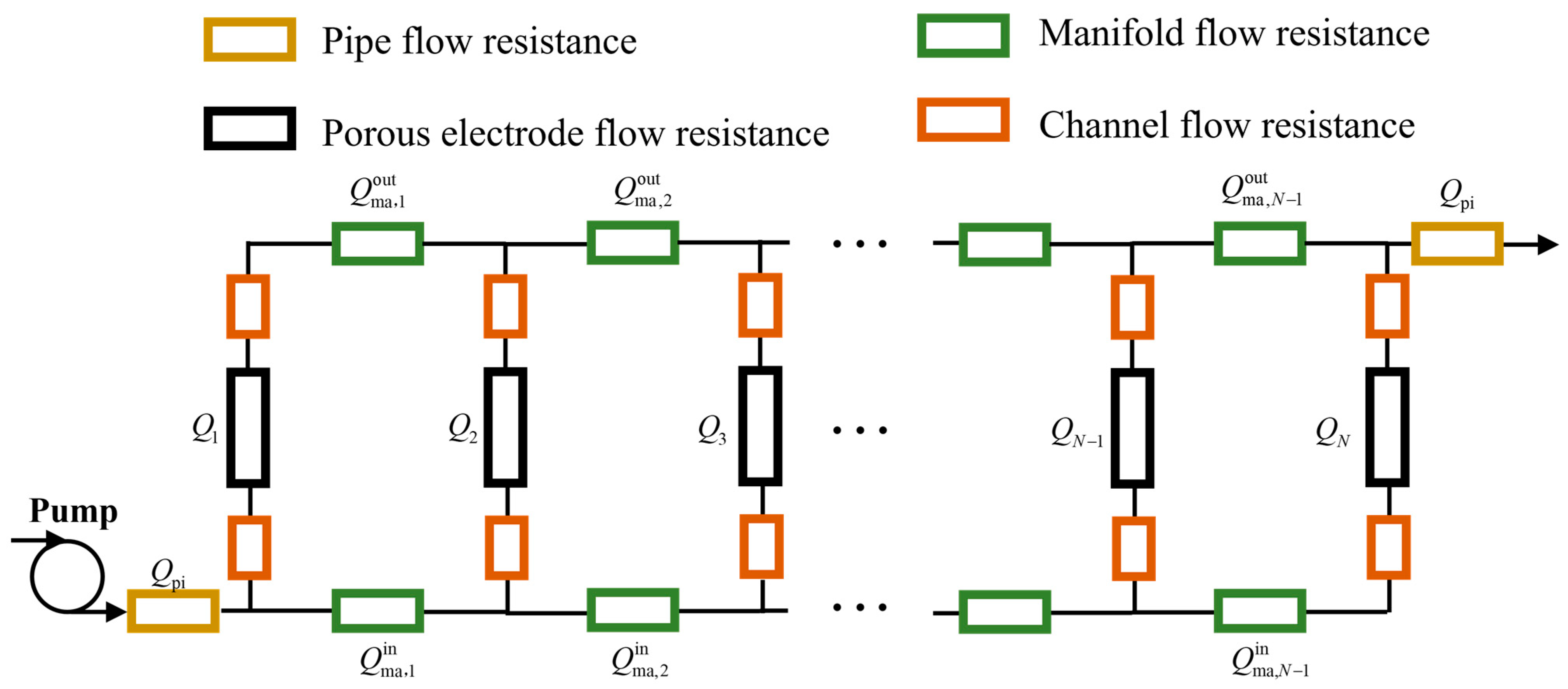
2.2. Electrolyte Flow Network Model

The electrolyte in the tank is first pumped into the external pipes, and then, the electrolyte in the external pipes is distributed to the individual cell via manifolds and channels in the flow frame, which results in different flow rates between cells. In order to calculate the flow rate of cells, the electrolyte flow network is exhibited in Figure 1. The electrolyte flow and pressure drop in the flow frame submit to Kirchhoff’s law, where the electrolyte flow rate is analogous to the current, the pressure drop is analogous to the voltage and the flow resistance is analogous to the electrical resistance.

As shown in Figure 1, in the electrolyte flow loop, there are four types of components: pipe, manifold, channel and porous electrode. The electrolyte flow rate and resistance in the pipe are denoted by $Q_{\mathrm{pipe}}$ and $R{f}_{\mathrm{pipe}}$ separately. The flow rate in the inlet manifold and outlet manifold are denoted by $Q_{\mathrm{ma},n}^{\mathrm{in}}$ and $Q_{\mathrm{ma},n}^{\mathrm{out}}$ separately, and the flow resistance in the inlet manifold and outlet manifold are denoted by $R{f}_{\mathrm{ma},n}^{\mathrm{in}}$ and $R{f}_{\mathrm{ma},n}^{\mathrm{out}}$ separately. The flow rates of the channel and electrode are the same in the same cell and denoted as $Q_n$. The flow resistances of the channel and electrode are denoted by $R{f}_{\mathrm{ch},n}$ and $R{f}_{e,n}$ separately. Assuming N cells in the stack, according to Kirchhoff’s current law, the electrolyte flow rate can be expressed as follows [2]:

$$\left\{\begin{array}{c}{Q}_1+Q_{\mathrm{ma},1}^{\mathrm{in}}=Q_{\mathrm{pipe}}\hfill \\ Q_1=Q_{\mathrm{ma},1}^{\mathrm{out}}\hfill \end{array}\right., n=1$$

$$\left\{\begin{array}{c}{Q}_n+Q_{\mathrm{ma},n}^{\mathrm{in}}=Q_{\mathrm{ma},n-1}^{\mathrm{in}}\hfill \\ Q_{\mathrm{ma},n-1}^{\mathrm{out}}+Q_n=Q_{\mathrm{ma},n}^{\mathrm{out}}\hfill \end{array}\right., 2\le n\le N-1$$

$$\left\{\begin{array}{c}{Q}_N=Q_{\mathrm{ma},N-1}^{\mathrm{in}}\hfill \\ Q_{\mathrm{ma},N-1}^{\mathrm{out}}+Q_N=Q_{\mathrm{pipe}}\hfill \end{array}\right., n=N$$

(16)

According to Kirchhoff’s voltage law, the pressure drop can be expressed as follows:

$$2\Delta P_{\mathrm{ch},n}+\Delta P_{e,n}+\Delta P_{\mathrm{ma},n}^{\mathrm{out}}=\Delta P_{\mathrm{ma},n}^{\mathrm{in}}+2\Delta P_{\mathrm{ch},n+1}+\Delta P_{\mathrm{e},n+1}, n=1\sim N-1$$

(17)

where $\Delta P_{\mathrm{ch}}$ and $\Delta P_e$ are the pressure drop of the channel and electrode, respectively; $\Delta P_{\mathrm{ma}}^{\mathrm{out}}$ and $\Delta P_{\mathrm{ma}}^{\mathrm{in}}$ are the pressure drop of the inlet manifold and outlet manifold, respectively.

The interconnection of the pressure drop ($\Delta P$), flow rate ($Q$) and flow resistance ($Rf$) is delineated by the following equation:

$$\Delta P=Q\cdot Rf$$

(18)

Therefore, Equation (17) can be rewritten with Equation (19) using the flow rate and flow resistance:

$$\begin{array}{l}{Q}_n(2R{f}_{\mathrm{ch},n}+R{f}_{e,n})+Q_{\mathrm{ma},n}^{\mathrm{out}}R{f}_{\mathrm{ma},n}^{\mathrm{out}}=Q_{\mathrm{ma},n}^{\mathrm{in}}R{f}_{\mathrm{ma},n}^{\mathrm{in}}\\ +Q_{n+1}(2R{f}_{\mathrm{ch},n+1}+R{f}_{e,n+1}), n=1\sim N-1\end{array}$$

(19)

In the pipe, manifold and channel, the electrolyte flow is considered laminar. The pressure drop is caused by friction and is calculated by the Darcy–Weisbach equation [21]:

$$\Delta P_f={\displaystyle \frac{f}{2}}\cdot {\displaystyle \frac{L}{D_{\mathrm{hc}}}}\cdot \rho \cdot ({\displaystyle \frac{Q}{A}}{)}^2$$

(20)

where $\Delta P_f$ is the pressure drop caused by friction, $f$ is the Darcy friction factor, $\rho$ is the density of the electrolyte, and $L$, $D_h$ and $A$ represent the length, hydraulic diameter and cross-sectional area of the pipe, manifold and channel as shown in Table 1. $f$ is expressed by the following equation [19]:

$$f={\displaystyle \frac{C}{Re}}, Re<2000,$$

$$\mathrm{in}\mathrm{which} \mathrm{C}=\left\{\begin{array}{c}64,\mathrm{f}\mathrm{o}\mathrm{r} \mathrm{c}\mathrm{i}\mathrm{r}\mathrm{c}\mathrm{u}\mathrm{l}\mathrm{a}\mathrm{r} \mathrm{s}\mathrm{e}\mathrm{c}\mathrm{t}\mathrm{i}\mathrm{o}\mathrm{n}\hfill \\ 55.5+40.9\times 0.03^{H/W},\mathrm{f}\mathrm{o}\mathrm{r} \mathrm{r}\mathrm{e}\mathrm{c}\mathrm{t}\mathrm{a}\mathrm{n}\mathrm{g}\mathrm{u}\mathrm{l}\mathrm{a}\mathrm{r} \mathrm{s}\mathrm{e}\mathrm{c}\mathrm{t}\mathrm{i}\mathrm{o}\mathrm{n}\hfill \end{array}\right.$$

(21)

where $C$ is the friction coefficient, and $\mathrm{Re}$ is the Reynolds number, which is required to be less than 2000 in Equation (21). The flow rate of the model built in Section 3 is 0.15 L/s, and the Reynolds number is about 1750 in the pipe and manifold, and about 294 in the channel, which meets the requirements. The Reynolds number is defined as follows:

$$\mathit{Re}={\displaystyle \frac{\rho D_{h}Q}{\mu A}}$$

(22)

where $\mu$ is the dynamic viscosity of the electrolyte.

Combining Equations (20)–(22), the relationship between the pressure drop, flow rate and flow resistance can be obtained as follows:

$$\Delta P_f={\displaystyle \frac{C\mu L}{2D_{\mathrm{hc}}^{2}A}}\cdot Q=R{f}_i\cdot Q_i, i=\mathrm{pi}, \mathrm{ch}, \mathrm{ma}$$

(23)

$$R{f}_i={\displaystyle \frac{C\mu L}{2D_{\mathrm{hc}}^{2}A}}, i=\mathrm{pi}, \mathrm{ch}, \mathrm{ma}$$

(24)

The electrolyte flow through the porous electrode is considered porous medium flow, and the pressure drop is calculated by Darcy’s law [2]:

$$\Delta P_e={\displaystyle \frac{\mu HQ}{KA}}$$

(25)

where $H$ and $A$ are the height and cross-sectional area of the porous electrode, as shown in Table 1, $Q$ is the electrolyte flow rate in the cell and $K$ is the permeability of the porous electrode that can be expressed by the Carman–Kozeny equation as follows:

$$K={\displaystyle \frac{d_f^2{\epsilon }^3}{K_{\mathrm{CK}}(1-\epsilon {)}^2}}$$

(26)

where $d_f$ is the carbon fiber diameter, $\epsilon$ is the porosity of the porous electrode and $K_{\mathrm{CK}}$ is the Carman–Kozeny constant.

Combining Equations (25) and (26), the relationship between the pressure drop, flow rate and flow resistance can be obtained as follows:

$$\Delta P_{\mathrm{e}}={\displaystyle \frac{K_{\mathrm{CK}}(1-\epsilon {)}^2}{d_f^2{\epsilon }^3}}\cdot {\displaystyle \frac{\mu H}{A}}\cdot Q=R{f}_{\mathrm{e}}\cdot Q$$

(27)

$$R{f}_{\mathrm{e}}={\displaystyle \frac{K_{\mathrm{CK}}(1-\epsilon {)}^2}{d_f^2{\epsilon }^3}}\cdot {\displaystyle \frac{\mu H}{A}}$$

(28)

2.3. Shunt Current

The flow of the conductive electrolyte leads to the generation of shunt currents, which flow in the manifolds and channels. The shunt currents can be represented by the equivalent circuit model, as displayed in Figure 2, where $E_{\mathrm{cell}}$ is the voltage of a single cell, as stated in Section 2.4. This equivalent circuit model is symmetric, so only half of the model needs to be computed to obtain the value of the shunt currents. Based on Kirchhoff’s current law, the following equations are established to calculate the shunt currents [2,3,12]:

$$\left\{\begin{array}{c}{I}_{\mathrm{app}}-I_{\mathrm{cell},1}-2I_{\mathrm{ch},1}^{+}=0\hfill \\ I_{\mathrm{ch},1}^{+}-I_{\mathrm{ma},1}^{+}=0\hfill \end{array}\right., n=1$$

(29)

$$\left\{\begin{array}{c}{I}_{\mathrm{cell},1}-I_{\mathrm{cell},2}-2I_{\mathrm{ch},2}^{+}-2I_{\mathrm{ch},1}^{-}=0\hfill \\ I_{\mathrm{ch},2}^{+}+I_{\mathrm{ma},1}^{+}-I_{\mathrm{ma},2}^{+}=0\hfill \\ I_{\mathrm{ch},1}^{-}-I_{\mathrm{ma},1}^{-}=0\hfill \end{array}\right., n= 2$$

(30)

$$\left\{\begin{array}{c}{I}_{\mathrm{cell},n-1}-I_{\mathrm{cell},n}-2I_{\mathrm{ch},n}^{+}-2I_{\mathrm{ch},n-1}^{-}=0\hfill \\ I_{\mathrm{ch},n}^{+}+I_{\mathrm{ma},n-1}^{+}-I_{\mathrm{ma},n}^{+}=0\hfill \\ I_{\mathrm{ch},n-1}^{-}+I_{\mathrm{ma},n-2}^{-}-I_{\mathrm{ma},n-1}^{-}=0\hfill \end{array}\right., 3\le n\le N-1$$

(31)

$$\left\{\begin{array}{c}{I}_{\mathrm{cell},N-1}-I_{\mathrm{cell},N}-2I_{\mathrm{ch},N}^{+}-2I_{\mathrm{ch},N-1}^{-}=0\hfill \\ I_{\mathrm{ch},N-1}^{-}+I_{\mathrm{ma},N-2}^{-}-I_{\mathrm{ma},N-1}^{-}=0\hfill \\ I_{\mathrm{ch},N}^{-}+I_{\mathrm{ma},N-1}^{-}=0\hfill \\ I_{\mathrm{cell},N}-2I_{\mathrm{ch},N}^{-}-I_{\mathrm{app}}=0\hfill \end{array}\right., n=N$$

(32)

where $I_{\mathrm{app}}$ is the applied current, $I_{\mathrm{cell}}$ is the current of the cell, and $I_{\mathrm{ch}}$ and $I_{\mathrm{ma}}$ are the shunt currents of the channels and manifolds. Based on Kirchhoff’s voltage law, the following equations are established:

$$E_{\mathrm{cell},1}-R_{\mathrm{ch},1}^{+}{I}_{\mathrm{ch},1}^{+}-R_{\mathrm{ma},1}^{+}{I}_{\mathrm{ma},1}^{+}+R_{\mathrm{ch},2}^{+}{I}_{\mathrm{ch},2}^{+}=0, n=1$$

(33)

$$\left\{\begin{array}{c}{E}_{\mathrm{cell},n}-R_{\mathrm{ch},n}^{+}{I}_{\mathrm{ch},n}^{+}-R_{\mathrm{ma},n}^{+}{I}_{\mathrm{ma},n}^{+}+R_{\mathrm{ch},n+1}^{+}{I}_{\mathrm{ch},n+1}^{+}=0\hfill \\ E_{\mathrm{cell},n}-R_{\mathrm{ch},n-1}^{-}{I}_{\mathrm{ch},n-1}^{-}-R_{\mathrm{ma},n-1}^{-}{I}_{\mathrm{ma},n-1}^{-}+R_{\mathrm{ch},n}^{-}{I}_{\mathrm{ch},n}^{-}=0\hfill \end{array}\right., 2\le n\le N-1$$

(34)

$$E_{\mathrm{cell},N}-R_{\mathrm{ch},N-1}^{-}{I}_{\mathrm{ch},N-1}^{-}-R_{\mathrm{ma},N-1}^{-}{I}_{\mathrm{ma},N-1}^{-}+R_{\mathrm{ch},N}^{-}{I}_{\mathrm{ch},N}^{-}=0, n=N$$

(35)

where $E_{\mathrm{cell}}$ is the voltage of the cell, and $R_{\mathrm{ch}}$ and $R_{\mathrm{ma}}$ are the resistance of the channels and manifolds.

The resistance of the manifolds and channels is related to the SOC and based on Ohm’s law:

$$R={\displaystyle \frac{L}{\sigma A}}$$

(36)

where $L$ and $A$ are the length and cross-sectional area of the manifold and channels, respectively, as shown in Table 1, and $\sigma$ is the electrolyte conductivity, which is calculated separately in the positive and negative side [3]:

$${\sigma }_{+}={\sigma }_4+\mathrm{SOC}({\sigma }_5-{\sigma }_4)$$

(37)

$${\sigma }_{-}={\sigma }_3+\mathrm{SOC}({\sigma }_2-{\sigma }_3)$$

(38)

where SOC is the state of charge of the VRFB.

2.4. Electrochemical Reaction

The cell voltage is determined by the open-circuit voltage (OCV) $E_{\mathrm{OCV}}$ and overpotential $\eta$:

$$E_{\mathrm{cell}}=E_{\mathrm{OCV}}-\eta$$

(39)

The OCV is derived from the Nernst equation:

$$E_{\mathrm{OCV}}=E_0+{\displaystyle \frac{RT}{zF}}\mathit{ln}(c_{{\mathrm{H}}^{+}}^2)+{\displaystyle \frac{RT}{zF}}\mathit{ln}({\displaystyle \frac{c_2{c}_5}{c_3{c}_4}})$$

(40)

$$E_0^{\prime }=E_0+{\displaystyle \frac{RT}{zF}}\mathit{ln}(c_{{\mathrm{H}}^{+}}^2)$$

(41)

where $E_0$ is the standard reversible potential, $E_0^{\prime }$ is the corrected standard reversible potential, which is considered 1.4 V according to [3,10,14], $R$ is the gas constant and $T$ is the temperature of the cell.

The overpotential consists of the ohmic overpotential, the concentration overpotential (${\eta }_c$) and the activation overpotential (${\eta }_a$):

$$\eta =I_{\mathrm{cell}}{R}_{\mathrm{cell}}+{\eta }_c^{+}+{\eta }_c^{-}+{\eta }_a^{+}+{\eta }_a^{-}$$

(42)

Owing to the concentration gradient and transport resistance of the active species in the electrolyte, the concentration overpotential occurs, which is calculated as follows [22]:

$${\eta }_c^{+}={\displaystyle \frac{RT}{zF}}\mathit{ln}(1-{\displaystyle \frac{i}{zF{k}_m{c}^{+}}})$$

(43)

$${\eta }_c^{-}={\displaystyle \frac{RT}{zF}}\mathit{ln}(1-{\displaystyle \frac{i}{zF{k}_m{c}^{-}}})$$

(44)

where $i$ is the current density of the cell, $c$ is the reactant concentration of the cell, $c^{+}$ is the concentration of $\mathrm{V}{\mathrm{O}}^{2+}/\mathrm{V}{\mathrm{O}}_2^{+}$ in the charging/discharging process, $c^{-}$ is the concentration of ${\mathrm{V}}^{3+}/{\mathrm{V}}^{2+}$ in the charging/discharging process and $k_m$ is the mass transfer coefficient which is calculated as follows [22]:

$$k_m=1.6\times 10^{-4}{\left({\displaystyle \frac{Q}{A}}\right)}^{0.4}$$

(45)

The activation overpotential results from the slow electrochemical reactions; however, the ${\eta }_a$ of the VRFB with porous electrodes is significantly reduced owing to the large active surface area. The ${\eta }_a$ is typically derived by the Bulter–Volmer equation.

The exchange current density of the positive and negative electrodes is calculated as follows [23]:

$$i_0^{+}=F{k}^{+}{c}_4^{(1-{\alpha }^{+})}{c}_5^{{\alpha }^{+}}$$

(46)

$$i_0^{-}=F{k}^{-}{c}_2^{(1-{\alpha }^{-})}{c}_3^{{\alpha }^{-}}$$

(47)

where $k^{+}$ and $k^{-}$ are the standard rate constant for the positive and negative electrodes, respectively; the transfer coefficient for positive (${\alpha }^{+}$) and negative (${\alpha }^{-}$) is 0.5 in this model [23]. Thus, the calculation equation for the activating overpotential is as follows [23,24,25]:

$${\eta }_a^{+}={\displaystyle \frac{2RT}{F}}\left[{\mathit{sinh}}^{-1}({\displaystyle \frac{i}{2F{k}^{+}\sqrt{c_4{c}_5}}})\right]$$

(48)

$${\eta }_a^{-}={\displaystyle \frac{2RT}{F}}\left[{\mathit{sinh}}^{-1}({\displaystyle \frac{i}{2F{k}^{-}\sqrt{c_2{c}_3}}})\right]$$

(49)

The ohmic overpotential is caused by current flowing through the resistance in the cell. The ohmic resistance includes the electrode resistance ($R_e$), membrane resistance ($R_m$), contact resistance ($R_{\mathrm{con}}$) and positive/negative electrolyte resistance ($R_{\mathrm{el}}^{\pm }$) [2]:

$$R_{\mathrm{cell}}=2R_{\mathrm{e}}+R_{\mathrm{m}}+2R_{\mathrm{con}}+R_{\mathrm{el}}^{+}+R_{\mathrm{el}}^{-}$$

(50)

The electrode resistance, membrane resistance and positive and negative electrolyte resistance obey Ohm’s law:

$$R_{\mathrm{e}}={\displaystyle \frac{1}{{\sigma }_{\mathrm{e}}(1-\epsilon {)}^{1.5}}}{\displaystyle \frac{L_{\mathrm{e}}}{W_{\mathrm{e}}{H}_{\mathrm{e}}}}$$

(51)

$$R_{\mathrm{m}}={\displaystyle \frac{1}{{\sigma }_{\mathrm{m}}}}{\displaystyle \frac{d}{W_{\mathrm{m}}{H}_{\mathrm{m}}}}$$

(52)

$$R_{\mathrm{el}}^{\pm }={\displaystyle \frac{1}{{\sigma }_{\mathrm{el}}^{\pm }{\epsilon }^{1.5}}}{\displaystyle \frac{L_{\mathrm{e}}}{W_{\mathrm{e}}{H}_{\mathrm{e}}}}$$

(53)

where $L_e$, $W_e$ and $H_e$ are the length, width and height of the electrode, $d$, $W_m$ and $H_m$ are the length, width and height of the membrane, as shown in Table 1, ${\sigma }_e$ and ${\sigma }_m$ are the conductivity of the electrode and membrane, and ${\sigma }_{\mathrm{el}}^{\pm }$ is calculated from the conductivity of all ions [2]:

$${\sigma }_{\mathrm{el}}^{+}={\displaystyle \frac{F^2}{RT}}\sum z_i^2{D}_i{c}_i, i= \mathrm{V}{\mathrm{O}}^{2+}, \mathrm{V}{\mathrm{O}}_2^{+}, \mathrm{S}{\mathrm{O}}_4^{2-},{\mathrm{H}}^{+}$$

(54)

$${\sigma }_{\mathrm{el}}^{-}={\displaystyle \frac{F^2}{RT}}\sum z_i^2{D}_i{c}_i, i={\mathrm{V}}^{2+},{\mathrm{V}}^{3+}, \mathrm{S}{\mathrm{O}}_4^{2-},{\mathrm{H}}^{+}$$

(55)

where $z_i$, $D_i$ and $c_i$ are the charge number, diffusion and concentration of ion $i$. The contact resistance can be obtained from experimental data [26].

2.5. Energy Balance

The heat in a VRFB system derives from heat sources and heat transfer. The heat sources contain the heat generation of the electrochemical reactions, ohmic resistance, crossover reaction and hydraulic friction. Heat transfer occurs between a VRFB system and the environment through the stack, inlet and outlet pipe and storage tanks.

Assuming the same temperature between the negative and positive electrodes in a single cell, the temperature of the n-th cell can be represented by $T_n$. The temperature variation of the n-th cell is as follows:

$$2\rho C_p{V}_e{\displaystyle \frac{d{T}_n}{dt}}=q_{re}+q_{oh}+q_{co}+q_{hf}+q_{tr}+q_{ef}$$

(56)

where $C_p$ is the electrolyte’ specific heat capacity, $\rho$ is the electrolyte density, $q_{re}$, $q_{oh}$, $q_{co}$ and $q_{hf}$ are the heat generation rate of the electrochemical reversible reaction, ohmic resistance, crossover reaction and hydraulic friction separately, and $q_{tr}$ and $q_{ef}$ are the heat transfer rate of convection and electrolyte flow separately.

$q_{re}$ is calculated by the following [11]:

$$q_{re}=I_n{T}_n{\displaystyle \frac{d{E}_{\mathrm{cell},n}}{d{T}_n}}$$

(57)

$${\displaystyle \frac{d{E}_{\mathrm{cell},n}}{d{T}_n}}={\displaystyle \frac{\Delta S^{\Theta }+R\mathit{ln}(\frac{c_{2,n}{c}_{5,n}{c}_{{\mathrm{H}}^{+},n}^2}{c_{3,n}{c}_{4,n}})}{zF}}$$

(58)

where $\Delta S^{\Theta }$ is the entropy change of the electrochemical reaction. Owing to the different reactants and products involved in the charge–discharge process, the heat rate is the opposite. $\Delta S^{\Theta }$ is derived as follows:

$$\Delta S=\sum S_{\mathrm{products}}^{\Theta }-\sum S_{\mathrm{reactants}}^{\Theta }$$

(59)

$$\Delta S^{\Theta }=S_{{\mathrm{V}}^{2+}}+S_{\mathrm{V}{\mathrm{O}}_2^{+}}^{\Theta }+2S_{{\mathrm{H}}^{+}}^{\Theta }-S_{\mathrm{V}{\mathrm{O}}^{2+}}^{\Theta }-S_{{\mathrm{V}}^{3+}}^{\Theta }-S_{{\mathrm{H}}_2\mathrm{O}}^{\Theta }, \mathrm{for} \mathrm{charging}$$

(60)

$$\Delta S^{\Theta }=S_{\mathrm{V}{\mathrm{O}}^{2+}}^{\Theta }+S_{{\mathrm{V}}^{3+}}^{\Theta }+S_{{\mathrm{H}}_2\mathrm{O}}^{\Theta }-S_{{\mathrm{V}}^{2+}}^{\Theta }-S_{\mathrm{V}{\mathrm{O}}_2^{+}}^{\Theta }-2S_{{\mathrm{H}}^{+}}^{\Theta }, \mathrm{for} \mathrm{discharging}$$

(61)

where $S^{\Theta }$ is the entropy of different species.

$q_{oh}$ is calculated by the following:

$$q_{oh}=I_n^2{R}_{\mathrm{cell},n}$$

(62)

$q_{co}$ is calculated by the following [3]:

$$q_{co}=-{\displaystyle \frac{S}{d}}(k_2{c}_{2,n}\Delta H_{II}+k_3{c}_{3,n}\Delta H_{III}+k_4{c}_{4,n}\Delta H_{IV}+k_5{c}_{5,n}\Delta H_V)$$

(63)

where $\Delta H$ is the crossover chemical reaction enthalpy change of Equations (3)–(6).

The heat generation rate of hydraulic friction $q_{hf}$ can be obtained from [12]. The electrolyte flow rate for this model is 0.15 L/s; so, the positive and negative electrolyte flow results in a friction production rate of 8 W. Distributed to each cell, the friction heat production rate is 0.4 W.

In the energy balance equation, the last two terms are the heat transfer, wherein $q_{tr}$ is the heat transfer rate of convection; the equation of the n-th cell is as follows [12]:

$$\begin{gathered} q_{tr}=U_x{A}_x(T_2-T_1)+U_{end}{A}_{end}(T_{air}-T_1)+2U_y{A}_y(T_{air}-T_1) \\ +2U_z{A}_z(T_{air}-T_1)+2\rho C_p{Q}_1(T_{in}-T_1), n=1 \end{gathered}$$

(64)

$$\begin{gathered} q_{tr}=U_x{A}_x(T_{n+1}-T_n)+U_x{A}_x(T_{n-1}-T_n)+2U_y{A}_y(T_{air}-T_n) \\ +2U_z{A}_z(T_{air}-T_n)+2\rho C_p{Q}_n(T_{in}-T_n), n=2\sim N-1 \end{gathered}$$

(65)

$$\begin{gathered} q_{tr}=U_x{A}_x(T_{N-1}-T_N)+U_{end}{A}_{end}(T_{air}-T_N)+2U_y{A}_y(T_{air}-T_N) \\ +2U_z{A}_z(T_{air}-T_N)+2\rho C_p{Q}_n(T_{in}-T_N), n=N \end{gathered}$$

(66)

where $T_{air}$ is the temperature of the environment air; $U_y$, $U_x$, $U_z$ and $U_{end}$ are the heat transfer coefficients in the x, y, z and end directions. Due to one side of the cell at both ends exchanging heat with air, the heat exchange equation is different from that of the middle cells. The heat transfer of the electrolyte flow is calculated as follows:

$$q_{ef}=2\rho C_p{Q}_n(T_{\mathrm{in}}-T_n)$$

(67)

where $T_{\mathrm{in}}$ is the temperature of the electrolyte in the inlet pipe.

Considering the influence of natural convection on pipes and tanks, the electrolyte temperature in the pipes and tanks is calculated as follows:

$$T_{\mathrm{stack}}={\displaystyle \frac{{\sum }_{n=1}^N{Q}_n{T}_n}{Q_{\mathrm{pi}}}}$$

(68)

$$\rho C_p{V}_{\mathrm{pipe}}{\displaystyle \frac{d{T}_{\mathrm{out}}}{dt}}=\rho C_{p}Q(T_{\mathrm{stack}}-T_{\mathrm{out}})+U_{\mathrm{pipe}}{A}_{\mathrm{pipe}}(T_{\mathrm{air}}-T_{\mathrm{out}})$$

(69)

$$\rho C_p{V}_{\mathrm{tank}}{\displaystyle \frac{d{T}_{\mathrm{tank}}}{dt}}=\rho C_{p}Q(T_{\mathrm{out}}-T_{\mathrm{tank}})+U_{\mathrm{tank}}{A}_{\mathrm{tank}}(T_{\mathrm{air}}-T_{\mathrm{tank}})$$

(70)

$$\rho C_p{V}_{\mathrm{pipe}}{\displaystyle \frac{d{T}_{\mathrm{in}}}{dt}}=\rho C_{p}Q(T_{\mathrm{tank}}-T_{\mathrm{in}})+U_{\mathrm{pipe}}{A}_{\mathrm{pipe}}(T_{\mathrm{air}}-T_{\mathrm{in}})$$

(71)

where $T_{\mathrm{stack}}$ is the characteristic temperature of the stack, $V_{\mathrm{pipe}}$, $U_{\mathrm{pipe}}$ and $A_{\mathrm{pipe}}$ are the volume, heat transfer coefficient and surface area of the pipe, $T_{\mathrm{out}}$ and $T_{\mathrm{tank}}$ are the temperature of the electrolyte in the outlet pipe and tank, and $U_{\mathrm{tank}}$ and $A_{\mathrm{tank}}$ are the overall heat transfer coefficient and area of the tank. The data of the Section 2 are shown in

Table 2. The physical constants and parameters of this model.

Symbol	Parameter	Value
N	Number of cells	20
R	Gas constant	8.314 J mol−1 K−1
F	Faraday’s constant	96,485
c	Total vanadium concentration	1.7 mol L−1
Vtank	Volume of electrolyte in tank	100 L
Cp	Electrolyte specific heat capacity	3200 J kg−1 K−1 [12]
ρ	Density of electrolyte	1354 kg m−3 [12]
μ	Dynamic viscosity of electrolyte	4.928 × 10−3 Pa s [19]
k2	Transmembrane diffusion coefficient of V2+	8.768 × 10−12 m2 s−1 [15]
k3	Transmembrane diffusion coefficient of V3+	3.222 × 10−12 m2 s−1 [15]
k4	Transmembrane diffusion coefficient of VO2+	6.825 × 10−12 m2 s−1 [15]
k5	Transmembrane diffusion coefficient of VO2+	5.897 × 10−12 m2 s−1 [15]
D2	Diffusion coefficient of V2+	2.4 × 10−10 m2 s−1 [2]
D3	Diffusion coefficient of V3+	2.4 × 10−10 m2 s−1 [2]
D4	Diffusion coefficient of VO2+	3.9 × 10−10 m2 s−1 [2]
D5	Diffusion coefficient of VO2+	3.9 × 10−10 m2 s−1 [2]
$D_{{\mathrm{H}}^{+}}$	Diffusion coefficient of H+	9.312 × 10−9 m2 s−1 [2]
$D_{\mathrm{S}{\mathrm{O}}_4^{2-}}$	Diffusion coefficient of SO42−	1.065 × 10−9 m2 s−1 [2]
σ2	Conductivity of V2+	27.5 S m−1 [12]
σ3	Conductivity of V3+	17.5 S m−1 [12]
σ4	Conductivity of VO2+	27.5 S m−1 [12]
σ5	Conductivity of VO2+	41.3 S m−1 [12]
σe	Conductivity of electrode	1000 S m−1 [2]
σm	Conductivity of membrane	7.3 S m−1 [2]
ε	Porosity	0.87 [27]
df	Carbon fiber diameter	11.94 × 10−6 m [27]
KCK	Carman–Kozeny constant	4.89 [27]
k+	Standard rate constant of positive reaction	6.8 × 10−7 m s−1 [20]
k−	Standard rate constant of positive reaction	2.6 × 10−6 m s−1 [20]
Ux	Heat transfer coefficient of cell in direction x	21.67 W m−2 K−1 [12]
Uy	Heat transfer coefficient of cell in direction y	2.413 W m−2 K−1 [12]
Uz	Heat transfer coefficient of cell in direction z	1.376 W m−2 K−1 [12]
Uend	Heat transfer coefficient of end cell in direction x	2.877 W m−2 K−1 [12]
Upipe	Heat transfer coefficient of pipe	3.667 W m−2 K−1 [12]
Utank	Heat transfer coefficient of tank	5.734 W m−2 K−1 [12]
$S_{{\mathrm{V}}^{2+}}^{\Theta }$	Standard molar entropy of V2+	−130.0 J mol−1 K−1 [15]
$S_{{\mathrm{V}}^{3+}}^{\Theta }$	Standard molar entropy of V3+	−230.0 J mol−1 K−1 [15]
$S_{\mathrm{V}{\mathrm{O}}^{2+}}^{\Theta }$	Standard molar entropy of VO2+	−133.9 J mol−1 K−1 [15]
$S_{\mathrm{V}{\mathrm{O}}_2^{+}}^{\Theta }$	Standard molar entropy of VO2+	−42.3 J mol−1 K−1 [15]
$S_{{\mathrm{H}}_2\mathrm{O}}^{\Theta }$	Standard molar entropy of H2O	69.9 J mol−1 K−1 [15]
$S_{{\mathrm{H}}^{+}}^{\Theta }$	Standard molar entropy of H+	0 J mol−1 K−1 [15]
ΔHII	Enthalpy of reaction in Equation (3)	−220.03 kJ mol−1 [3]
ΔHIII	Enthalpy of reaction in Equation (4)	−64.40 kJ mol−1 [3]
ΔHIV	Enthalpy of reaction in Equation (5)	−91.23 kJ mol−1 [3]
ΔHV	Enthalpy of reaction in Equation (6)	−246.86 kJ mol−1 [3]

.

3. Model Validation and Physical Parameters Distribution

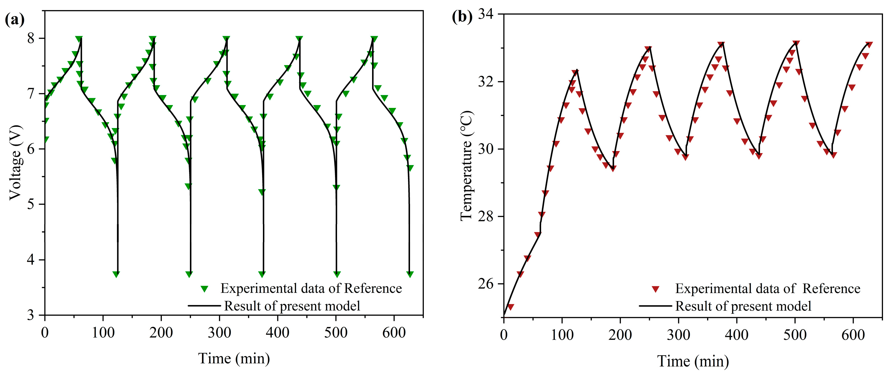
3.1. Model Validation

In order to prove the accuracy and reliability of the established multi-physics VRFB stack model in this work, the simulated voltage and temperature of a five-cell stack are compared with the experimental data [3] using the same operating conditions and geometric dimensions. The operating current density is 100 mA cm⁻², the electrolyte flow rate is 0.03 L/s, the ambient temperature is 25 °C and the cut-off voltages are 8.0 V and 3.75 V during the charging and discharging processes. As shown in Figure 3, the simulated charge–discharge voltage and temperature match well with the experimental data [3]. In this validation, the average error of voltage and temperature for the simulated and experimental results of the stack is 2.31% and 2.85%, respectively, which can prove that the established multi-physics VRFB stack model in this work is reliable and accurate.

It should be noted that the temperature increment of the stack during the charging process in the first cycle is higher than in later cycles, which is explained as follows. In the first cycle, the heat dissipation from the VRFB system to the outside air is small due to the same initial temperature. In later cycles, the heat dissipation from the VRFB system to the outside air is increased due to the increased VRFB system temperature.

In the following study, a stack with 20 single cells is established. The cut-off voltage of the stack is 33 V in the charging process and 23 V in the discharging process. The charging and discharging currents are 60 A and the total flow rate is 0.15 L s⁻¹.

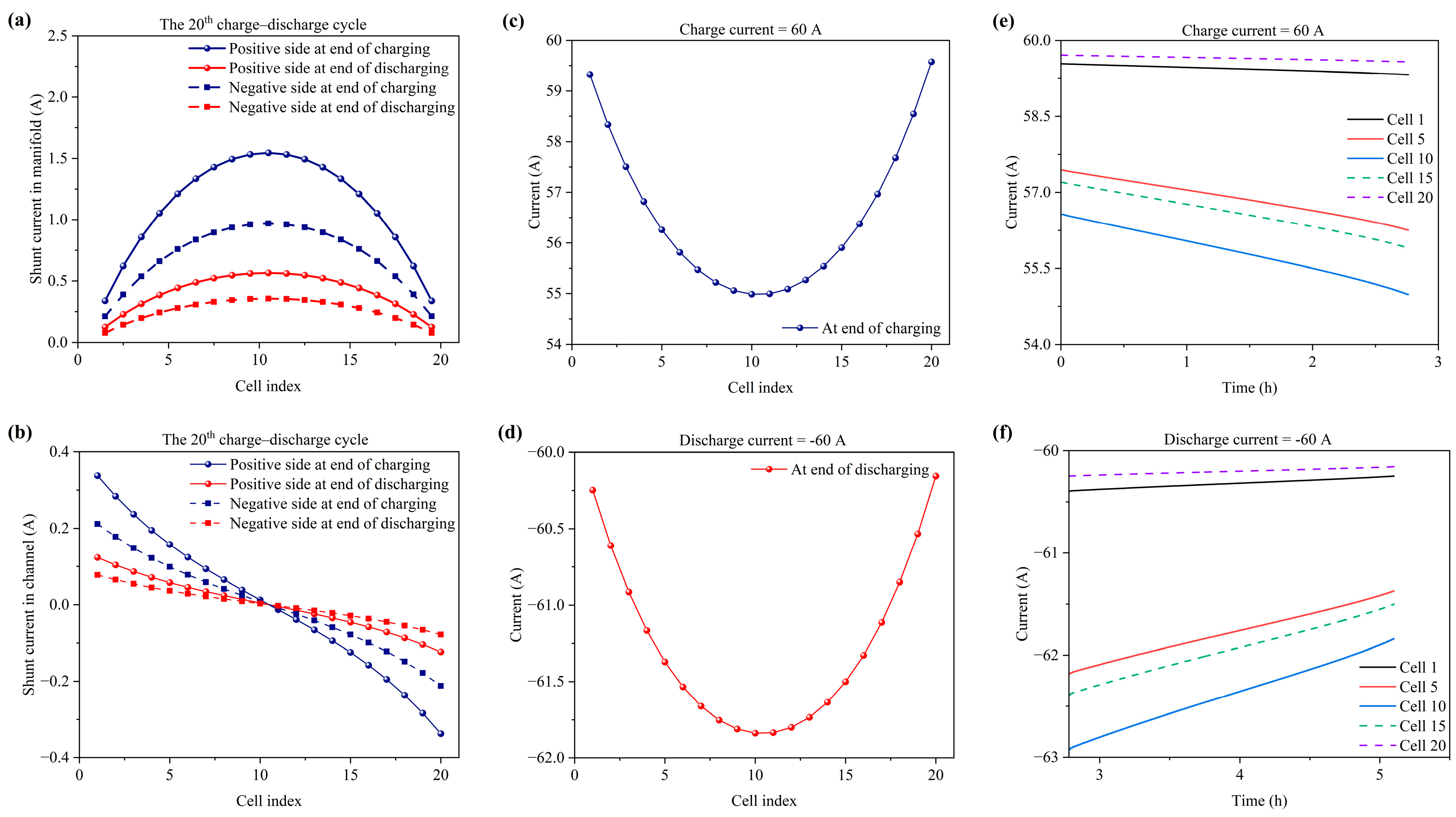
3.2. Flow Rate Distribution in Stack

Figure 4 shows the flow rate deviation of the cells in the 20-cell stack with a flow rate of 0.15 L s⁻¹. The flow rate deviation of the n-th cell represents the differences between the flow rate of the n-th cell and the average flow rate of the stack. The flow deviation is 1.92% in the first cell. With the cell index increasing, the flow deviation decreases initially. In particular, the flow deviation decreases to −1.11% at the 10th and 11th cells. With further increases in the cell index, the flow deviation increases. For the 20th cell, the flow deviation is increased to 1.92%, which is the same as that for the 1st cell. According to flow deviation variation, the following points can be concluded. Firstly, the flow rate is highest in the 1st cell and 20th cell for the reason that they are located near to the inlet and outlet, and the flow rate is lowest in the 10th and 11th cells due to the by-pass electrolyte flow in the frame and electrode. Secondly, the flow rate distribution is non-uniform across the cells in the stack. Thirdly, the flow rate distribution is symmetrical.

3.3. Current Variation and Distribution in Stack

Figure 5a,b show the shunt currents in the manifolds and channels at the end of charging and discharging for the 20th cycle with a current of 60 A. In Figure 5a,b, the positive value denotes the same direction as that marked in Figure 2 and the negative value represents the opposite direction to that marked in Figure 2. Shunt currents derive from the conductive electrolyte flowing in the manifolds and channels. From Figure 5a, it can be found that as the cell index increases, the shunt currents in the manifolds increase initially and then decrease, which is attributed to the accumulation of shunt currents in the channels (Figure 5a). From Figure 5b, it can be found that the shunt currents in the channels present a positive value (the same direction as that marked in Figure 2) from the first cell to the center cell, and a negative value (the opposite direction to that marked in Figure 2) from the center cell to the 20th cell, which is the reason for shunt current variation in the manifold (Figure 5a). As shown in Figure 2, the single cells are put in series and the total voltage of the stack is the sum of the voltage of single cells. In other words, the first cell possesses the highest potential, while the 20th cell holds the lowest potential, which results in shunt current direction variation in the channels with the increase in the cell index (Figure 5b).

Moreover, as shown in Figure 5a, the shunt currents in the manifolds show a higher ramping rate at the 1st and 20th cells but exhibit a lower ramping rate at the center cells, which is in accordance with the shunt current magnitude in the channels (Figure 5b). Moreover, as shown in Figure 5a, it can be found that the shunt currents in the positive side are higher than those in the negative side at the end of both charging and discharging, which can be attributed to the lower electric resistance of the positive side. Similarly, as shown in Figure 5b, the shunt currents in the channels present the same pattern.

Figure 5c,d show the current variation across single cells in the stack at an applied current of 60 A in the 20th charge–discharge cycle. From Figure 5c,d, it can be found that the current magnitude of single cells during the charging process is lower than the applied current (60 A), while the current magnitude of single cells during the discharging process is larger than the applied current, which is attributed to the positive direction of shunt currents in the manifolds (Figure 5a and Figure 2). In addition, the current magnitude of single cells is decreased initially and then increased during the charging process, while the current magnitude of single cells is increased initially and then decreased during the discharging process, which is in accordance with the shunt current variation in the manifolds and channels (Figure 5a,b).

Figure 5e,f exhibit cell current variation during the charging process and discharging process separately at a current of 60 A. With the charging proceeding, the cell current is decreased gradually, which is attributed to the gradually decreased electric resistance in the manifolds and channels. Similarly, with the discharging proceeding, the cell current magnitude is decreased due to the gradually increased electric resistance in the manifolds and channels.

3.4. Voltage Variation and Distribution in Stack

Figure 6a exhibits the single-cell voltage variation in the charge–discharge process at a current of 60 A in the 20th cycle. Figure 6b exhibits the cell voltage distribution at the end of the charging and discharging process at a current of 60 A in the 20th cycle. It can be seen that the voltage distribution is almost symmetrical. Furthermore, it can be found that for the 1st and 20th cells, the cells possess the highest charging and discharging voltage due to having the highest cell current during charging and the lowest cell current during discharging (Figure 5). For the center cell, the cell shows the lowest charging and discharging voltage due to having the lowest cell current during charging and the highest cell current during discharging (Figure 5).

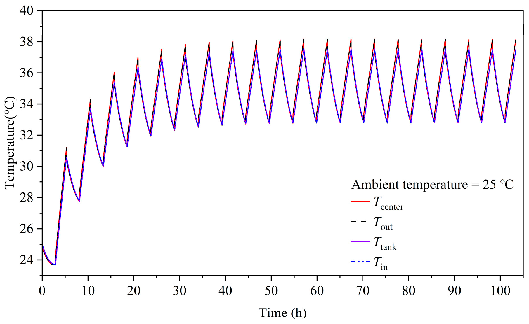
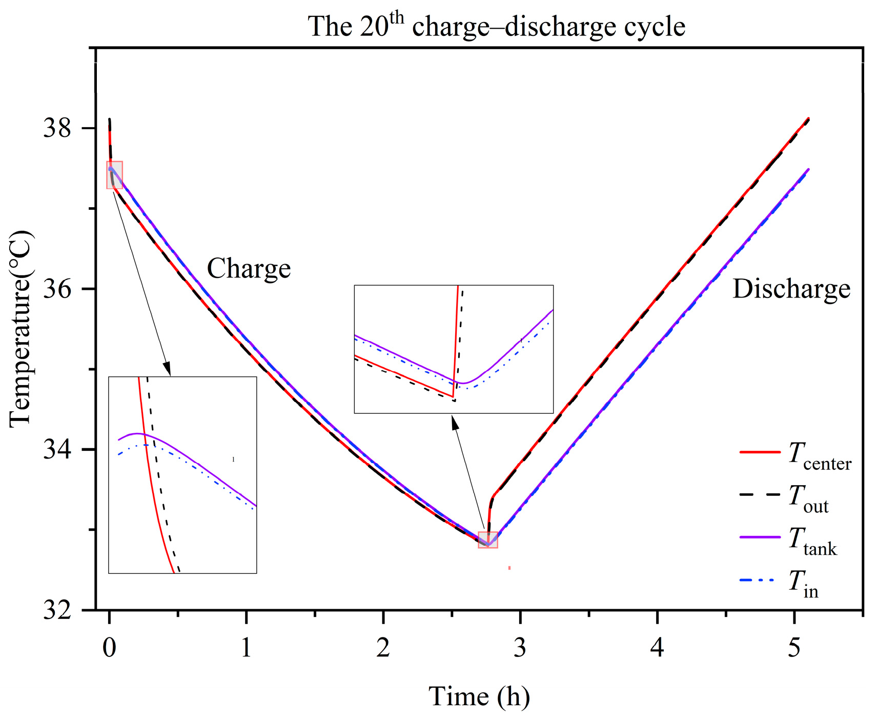
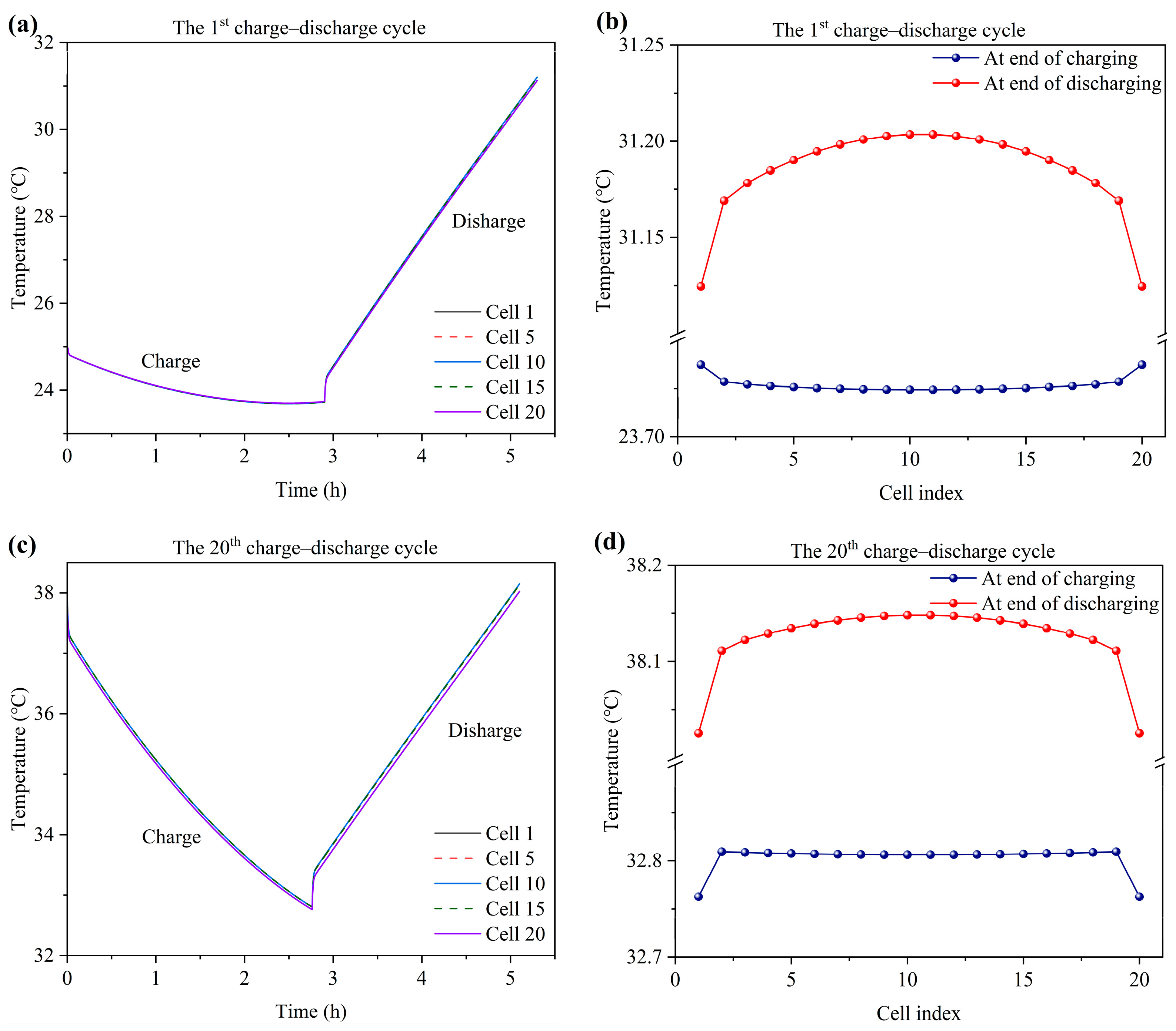
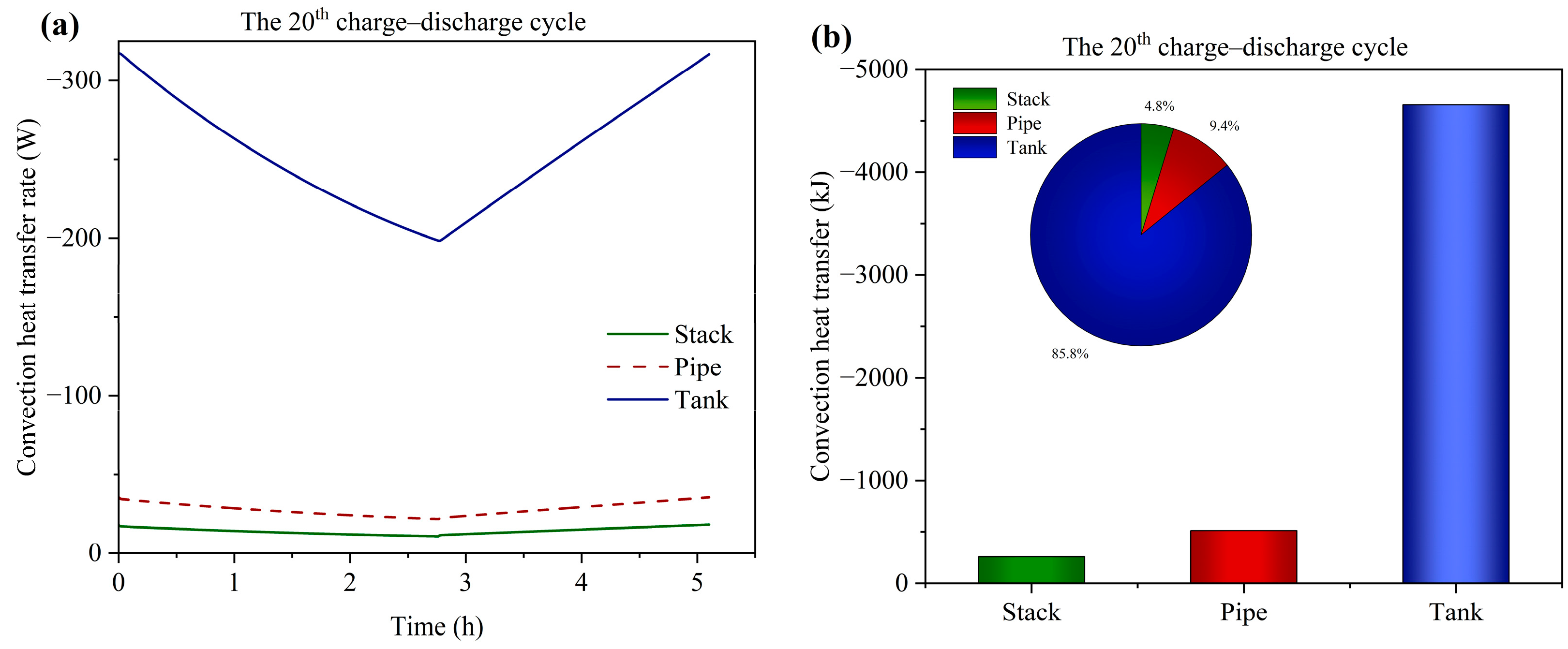
3.5. Temperature Variation and Distribution

Figure 7 shows the electrolyte temperature variation of the center cell (10th cell), outlet pipe, tank and inlet pipe during charge–discharge cycles at an ambient temperature of 25 °C. Because the temperature of the 10^th cell is highest in the stack, it was chosen for analysis. The temperature of the four components rises with time due to reversible heat generation and irreversible heat generation. After 20 charge–discharge cycles, the temperature gradually reaches a steady state, which can be explained as follows. The temperature increment of the cell, pipe and tank increases heat dissipation to the environment. The electrochemical charging reaction is an endothermic process. Increased heat dissipation and reversible heat absorption offset heat generation, which brings about a steady-state temperature.

Figure 8 shows the electrolyte temperature variation of the center cell (10th cell), outlet pipe, tank and inlet pipe during the 20th charge–discharge cycle. Owing to the small volume and surface area of the pipe, the heat transfer rate is low, so $T_{\mathrm{out}}$ is close to $T_{\mathrm{center}}$, and $T_{\mathrm{in}}$ is close to $T_{\mathrm{tank}}$. In the initial charging process, $T_{\mathrm{center}}$ drops rapidly, while the change in $T_{\mathrm{tank}}$ has a hysteresis, which experiences a short rising period due to the initial higher temperature of the center cell (stack). The electrolyte with the higher temperature in the stack flows into the tank and raises the tank temperature. When $T_{\mathrm{center}}$ decreases to a low level, $T_{\mathrm{tank}}$ will decrease simultaneously. It can also be found that $T_{\mathrm{tank}}$ is higher than $T_{\mathrm{center}}$, and the gap between $T_{\mathrm{tank}}$ and $T_{\mathrm{center}}$ gradually decreases. During the initial discharging process, $T_{\mathrm{center}}$ rises rapidly, while the variation in $T_{\mathrm{tank}}$ also has a hysteresis, which still declines for a short time before starting to rise. After the initial discharging process, $T_{\mathrm{tank}}$ is lower than $T_{\mathrm{center}}$, and the gap between $T_{\mathrm{tank}}$ and $T_{\mathrm{center}}$ gradually increases.

Figure 9a,c show the cell temperature variation during the 1st and 20th charge–discharge process at 60 A. In the charging process, the cell temperature drops due to the heat absorption of the electrochemical reversible reaction, while in the discharge process, the cell temperature rises owing to the heat generation of the electrochemical reversible reaction, heat generation from the ohmic resistance, hydraulic friction and self-discharge. Figure 9b,d show the temperature distribution across single cells at the 1st and 20th end of the charging and discharging process. The cell temperature distribution is symmetrical. In the charging process, the temperature difference of the middle cells is close and less than 0.01 °C. In the first charging process, the temperature of the 1st and 20th cell is obviously higher than that of the middle cells due to the temperature of the cells being lower than that of the environment (the cells absorb heat from the environment) and the large degree of heat absorption from the endplate to the environment. In the 20th charging process, the temperature of the 1st and 20th cell is obviously lower than that of the middle cells due to the temperature of the cells being higher than that of the environment (the cells dissipate heat into the environment) and the large degree of heat dissipation from the endplate to the environment. Similarly, during the discharging process, the temperature of the 1st and 20th cell is also lower than that of the middle cells. In the discharging process, the temperature difference of the cells is less than 0.1 °C.

Figure 10a and Figure 11a show the heat generation rate of the electrochemical reaction $q_{re}$ in the 1st and 20th charge–discharge cycle at a current of 60 A. Negative heat generation during charging indicates an endothermic process, while positive heat generation during discharging indicates an exothermic process. It can be found that the $q_{re}$ values of different single cells are almost the same as each other.

Figure 10b and Figure 11b show the heat generation rate of the ohmic resistance $q_{oh}$ in the 1st and 20th charge–discharge cycle at a current of 60 A. In the charging process, the $q_{oh}$ value of the 1st and 20th cells is higher than that of the 10th cell due to the lower current of the 10th cell. Similarly, due to the higher current of the 10th cell in the discharging process, the 10th cell presents a higher $q_{oh}$ than the 1st and 20th cells. In addition, for the reason that the relationship between the SOC and ohmic resistance is varied during the charge–discharge process, $q_{oh}$ is also changed.

Figure 10c and Figure 11c show the heat generation rate of the crossover reaction $q_{co}$ in the 1st and 20th charge–discharge cycle at a current of 60 A. It can be found that the $q_{co}$ values of different single cells are almost the same as each other in the charge–discharge process. Moreover, $q_{co}$ increases during the charging process but decreases during the discharging process, which is attributed to the different enthalpy changes of self-discharge reactions.

Figure 10d and Figure 11d show the heat transfer rate of convection $q_{tr}$ between the cell and environment in the 1st and 20th charge–discharge cycle at a current of 60 A. The $q_{tr}$ value of the 1st and 20th cells is much greater than that of the 10th cell due to the additional endplate heat dissipation to the environment. In the 1st charge and discharge cycle, $q_{tr}$ is positive in the first half of the stage, and then gradually decreases as the discharge process proceeds, because in the first half of the stage, the cell temperature is lower than the ambient temperature, and the cell absorbs heat from the environment. Then, as the cell temperature rises, the cell dissipates heat to the environment, and $q_{tr}$ becomes negative. In the 20th charge and discharge cycle, the cell temperature is always higher than the ambient temperature, and the cell dissipates heat to the environment; so, $q_{tr}$ always is negative.

Figure 10e and Figure 11e show the heat transfer rate of the electrolyte flow $q_{ef}$ between the cell and tank in the 1st and 20th charge–discharge cycle at a current of 60 A. For the reason that the storage tank temperature remains constant at the instantaneous alternating points between charging and discharging, the heat transfer rate of the electrolyte flow experiences a sharp increase and decrease at the start of the charge and discharge processes. Additionally, the heat transfer rate of the electrolyte flow is decreased during the charge process due to the decreased temperature difference between the cell and tank. Similarly, the magnitude of the heat transfer rate is increased during the discharge process due to the increased temperature difference between the cell and tank. Moreover, it can be found that the 10th cell exhibits a higher heat transfer rate than the 1st and 20th cell during the first charge process, because the temperature of the 10th cell is lower than the temperature of the 1st and 20th cell, the temperature difference between the 10th cell and the tank electrolyte is greater (the tank temperature is higher than the cell temperature), and the $q_{ef}$ value of the 10th cell is higher. While the 10th cell exhibits a lower heat transfer rate than the 1st and 20th cell during the 20th charge process because the temperature of the 10th cell is higher than the temperature of the 1st and 20th cell, the temperature difference between the 10th cell and the tank electrolyte is lower, and the $q_{ef}$ value of the 10th cell is lower. In the discharging process, because the temperature of the 10th cell is higher than the temperature of the 1st and 20th cell, the temperature difference between the 10th cell and the tank electrolyte is higher (the tank temperature is lower than the cell temperature) and the absolute value of $q_{ef}$ of the 10th cell is greater.

Figure 10f and Figure 11f show the total heat of single cells in the 1st and 20th charge–discharge cycle at a current of 60 A. It can be found that the total heat is negative in the charging process but is positive in the discharging process, which is in accordance with the temperature decrement and increment in the charging and discharging process. Furthermore, the 1st and 20th cells show a lower total heat compared to the middle cells, which is the cause of the temperature variation in Figure 9b,d.

Overall, the electrochemical reaction is the most influential factor in relation to the total heat of single cells. And the second most influential factor is the electrolyte flow heat transfer between the cell and tank. Heat generation from the ohmic resistance is an intermediate influencing factor in relation to the total heat of single cells. The least impactful factors are heat generation from the crossover reaction and convection heat transfer between the cell and environment.

The convective heat transfer between the VRFB system and the external environment is through stack, pipes and tanks. The heat transfer rate of tanks is much higher than that of pipes and the stack, as shown in Figure 12a. In the 20^th charge–discharge cycle, the convective transfer heat of stack, pipe and tank are 258.4, 512.1 and 4656.1 kJ respectively, and the total transfer heat ratio of the tank is as high as 85.8%, as shown in Figure 12b. Thus, the heat transfer of tanks dominates the convective heat transfer in the VRFB system.

Because the 10th cell has the highest temperature during discharging, the temperature of the 10th cell represents the stack temperature. Figure 13a shows the stack temperature variation of 20 charge–discharge cycles. It is shown that the stack temperatures have a similar variation pattern and reach equilibrium after 20 charge–discharge cycles for different ambient temperatures. In addition, it can be found that with increasing ambient temperature, the equilibrium temperature of the stack also increases. In particular, at an ambient temperature of 30 °C and 35 °C, the stack temperature will exceed the safe limit temperature of 40 °C; so, it is necessary to carry out cooling control to prevent the occurrence of thermal precipitation. Moreover, the equilibrium temperatures of the stack at different ambient temperatures are presented in Figure 13b. It can be seen that the increase rate of the equilibrium temperature is kept constant with varied ambient temperatures, which indicates the constant sensitivity of the stack temperature to ambient temperature.

4. VRFB Cooling Control Strategy

Excessively high temperatures (>40 °C) of the stack will lead to ${\mathrm{VO}}_2^{+}$ precipitation and blockage, which can result in the failed operation of the stack. To keep the stack temperature below 40 °C, effective cooling control is needed. In this section, a new tank cooling control strategy is presented to keep the temperature below 40 °C and achieve lower air conditioning energy consumption simultaneously.

4.1. Room Gas Flow Cooling Control Model

A room cooling control model is established to investigate the thermal dynamics and energy consumption of cooling control using air conditioning. The room is a space that contains the VRFB system and is surrounded by an external environment. Based on heat transfer between the external environment and the room ($q_{\mathrm{loss}}$ and $P_{\mathrm{loss}}$), heat transfer between the VRFB system and the room ($q_{\mathrm{heat}}$ and $P_{\mathrm{heat}}$), and the energy consumed to change the room temperature at the initial stage ($P_{\mathrm{ini}}$), the energy consumed by the air conditioning ($P_{\mathrm{ac}}$) can be calculated as follows [24,28,29]:

$$q_{\mathrm{loss}}=(T_{\mathrm{air}}-T_{\mathrm{room}})\cdot U_{\mathrm{wall}}\cdot A_{\mathrm{wall}}$$

(72)

$$P_{\mathrm{ini}}=M_{\mathrm{air}}\cdot C_{\mathrm{air}}\cdot (T_{\mathrm{air}}-T_{\mathrm{room}})$$

(73)

$$P_{\mathrm{loss}}=\int q_{\mathrm{loss}}dt$$

(74)

$$\begin{gathered} q_{\mathrm{heat}}=\left\{\begin{array}{c}{\displaystyle \sum _{n=1}^{20}}2\left(U_y{A}_y+U_z{A}_z\right)\left(T_n-T_{room}\right)+U_{end}{A}_{end}\left(T_1+T_2-2T_{room}\right)+2U_{pipe}{A}_{pipe}\hfill \\ \left(T_{out}+T_{in}-2T_{room}\right)+2U_{tank}{A}_{tank}\left(T_{tank}-T_{room}\right), \mathrm{f}\mathrm{o}\mathrm{r} \mathrm{c}\mathrm{o}\mathrm{m}\mathrm{m}\mathrm{o}\mathrm{n} \mathrm{s}\mathrm{t}\mathrm{r}\mathrm{a}\mathrm{t}\mathrm{e}\mathrm{g}\mathrm{y}\\ 2U_{tank}{A}_{tank}\left(T_{tank}-T_{room}\right), \mathrm{f}\mathrm{o}\mathrm{r} \mathrm{n}\mathrm{e}\mathrm{w} \mathrm{s}\mathrm{t}\mathrm{r}\mathrm{a}\mathrm{t}\mathrm{e}\mathrm{g}\mathrm{y}\end{array}\right. \\ {P}_{\mathrm{heat}}=\int q_{\mathrm{heat}}dt \end{gathered}$$

(75)

$$P_{\mathrm{ac}}={\displaystyle \frac{P_{\mathrm{ini}}+P_{\mathrm{loss}}+P_{\mathrm{heat}}}{EER}}$$

(76)

where $T_{\mathrm{air}}$ and $T_{\mathrm{room}}$ are the ambient and room temperatures, respectively, $U_{\mathrm{w}\mathrm{a}\mathrm{l}\mathrm{l}}$ and $A_{\mathrm{w}\mathrm{a}\mathrm{l}\mathrm{l}}$ are the heat transfer coefficient and surface of the concrete wall, respectively, and $M_{\mathrm{air}}$ and $C_{\mathrm{air}}$ are the mass and heat capacity of the air inside the room, respectively; the energy efficiency ratio ($EER$) is the refrigeration performance coefficient.

Moreover, the model is developed according to the following assumptions:

• The temperatures of the room ground and walls are the same.
• The air mass in the room remains constant.
• In the room, the VRFB system is the only heat source.
• The temperature of the room changes instantly in the initial stage.

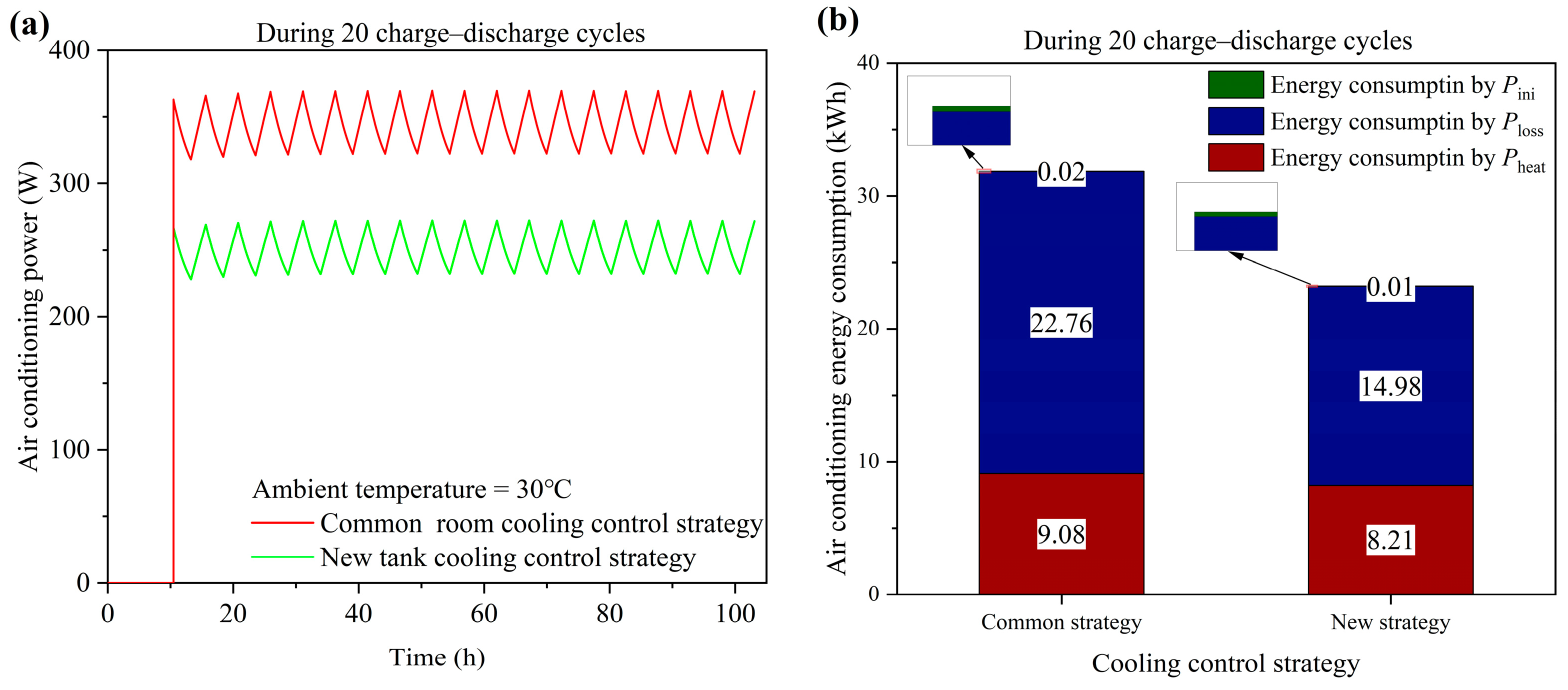
4.2. Common Room Cooling Control Strategy

The common room control strategy is to store the entire VRFB system including the stack, pipes and tanks in the same room for cooling control. Therefore, a sufficiently large room is needed to store the entire VRFB system for cooling control, and the parameters of this room are shown in

Table 3. Parameters of common and new strategy.

Symbol	Parameter	The Common Strategy	The New Strategy
H × L × W	Cooling control room dimension	3 m × 3 m × 2 m	2 m × 2 m × 2 m
Awall	Total surface of walls	42 m2	24 m2
Uwall	Total heat transfer coefficient of room	5.32 W m−2 K−1 [15]	5.32 W m−2 K−1 [15]
Cair	Heat capacity of air	1020 J kg−1 K−1	1020 J kg−1 K−1
Mair	Air mass inside cooling control room	23 kg	10 kg
EER	Energy efficiency ratio	3 [15]	3 [15]

.

As shown in Figure 13, when the ambient temperature is 30 °C and 35 °C, the temperature of the stack will exceed 40 °C, so it is necessary to employ cooling control to prevent the cell temperature from exceeding 40 °C. This work carried out cooling control at an ambient temperature of 30 °C.

Figure 14a shows the stack temperature variation without and with cooling control at an ambient temperature of 30 °C. It can be seen that without cooling control, the stack temperature will exceed 40 °C by 3.1 °C. The cooling control strategy is as follows: start controlling the temperature when the stack temperature exceeds 40 °C for the first time (during discharging of the third charge–discharge cycle) and control the room temperature at 26.9 °C. With the control strategy, the stack temperature is controlled so that it decreases on the whole; however, the stable temperature of the stack exceeds 40 °C by 0.2 °C. In addition, there is still a short period in which the stack temperature is higher than 40 °C. To keep the stack temperature below 40 °C exactly, the starting cooling point and controlled room temperature are adjusted. The results show that starting cooling at 38.5 °C during charging of the third charge–discharge cycle and controlling the room temperature at 26.7 °C are suitable strategies, as shown in Figure 14b.

4.3. New Tank Cooling Control Strategy

Since heat dissipation of the VRFB system mainly occurs through the tanks (Figure 12), a new tank cooling control strategy is proposed to keep the stack temperature below 40 °C and simultaneously decrease the energy consumption of the new strategy. The new tank cooling control strategy stores tanks in a room for cooling control and stores the stack in another room without cooling control that has large areas of ventilation windows around the walls, allowing air to flow in from the outside environment so the temperature of the room can be considered the same as the ambient temperature. Since only the cooling of the tanks is controlled, the volume of the room requiring temperature control can be reduced. The parameters of the tank room are shown in Table 3.

Based on the experience of the common room cooling control strategy, the start of the new tank cooling control strategy is at 38.5 °C during charging of the third charge–discharge cycle and the tank room temperature is controlled at 26.7 °C, as shown in Figure 14a.

When the new cooling strategy employs the same starting cooling points and controlled room temperature as that in the common room cooling control strategy, the maximum temperature of the stack is higher than 40 °C when the stack temperature reaches equilibrium. This is because the new tank cooling strategy only provides cooling control of the tanks and excludes the stack and pipes. By adjusting the controlled tank room temperature to 26.3 °C and keeping the starting cooling point at 38.5 °C, the stack temperature is always lower than 40 °C (Figure 15b), which indicates that the cooling control strategy is effective.

The power and energy consumption of the air conditioning are shown in Figure 16. In the cooling control process, the air conditioning power of the new tank strategy is always lower than that of the common room strategy. Therefore, during 20 charge–discharge cycles, compared to the common room cooling strategy, the new tank cooling control strategy can save 27.18% of air conditioning energy consumption. By exchanging the room temperature to a controlled temperature at the initial stage and allowing for heat transfer between the external environment and the room as well as heat transfer between the VRFB system and the room, the air conditioning energy consumption is, respectively, reduced by 50.00%, 34.18% and 9.58%. The result proves that the new tank cooling control strategy is more energy-efficient than the common room cooling strategy. Therefore, the new tank cooling control strategy has guiding significance for the future development of cooling control strategies.

5. Conclusions

In this work, a comprehensive multi-physics model is established for a 20-cell stack containing electrolyte flow, mass transport, electrochemical reactions, shunt currents, and heat generation and transfer. A new tank cooling strategy is proposed for maintaining the stack temperature below 40 °C. The major conclusions are as follows:

• The electrolyte flow rate exhibits non-uniform distribution across the cells in the stack. The end cells (1st and 20th cells) possess the highest flow rate and the center cell (10th and 11th cells) possesses the lowest flow rate.
• The shunt currents in the manifolds are largest at the center cell (10th and 11th cells) and lowest at the end cells (1st and 20th cells), and the shunt currents in the channels change direction across the cells in the stack, which can be attributed to the highest voltage of the 1st cell and the lowest voltage of the 20th cell in a series arrangement. In addition, the shunt currents in the positive side are higher than those in the negative side due to the lower resistance in the positive electrolyte.
• At the end of the charging and discharging process, the outermost end cells (1st and 20th cells) possess the lowest charging voltage and the highest discharging voltage due to having the highest flow rate and enough active species. The center cells (10th and 11th cells) show the worst charge–discharge performance due to having the lowest flow rate and a lack of active species.
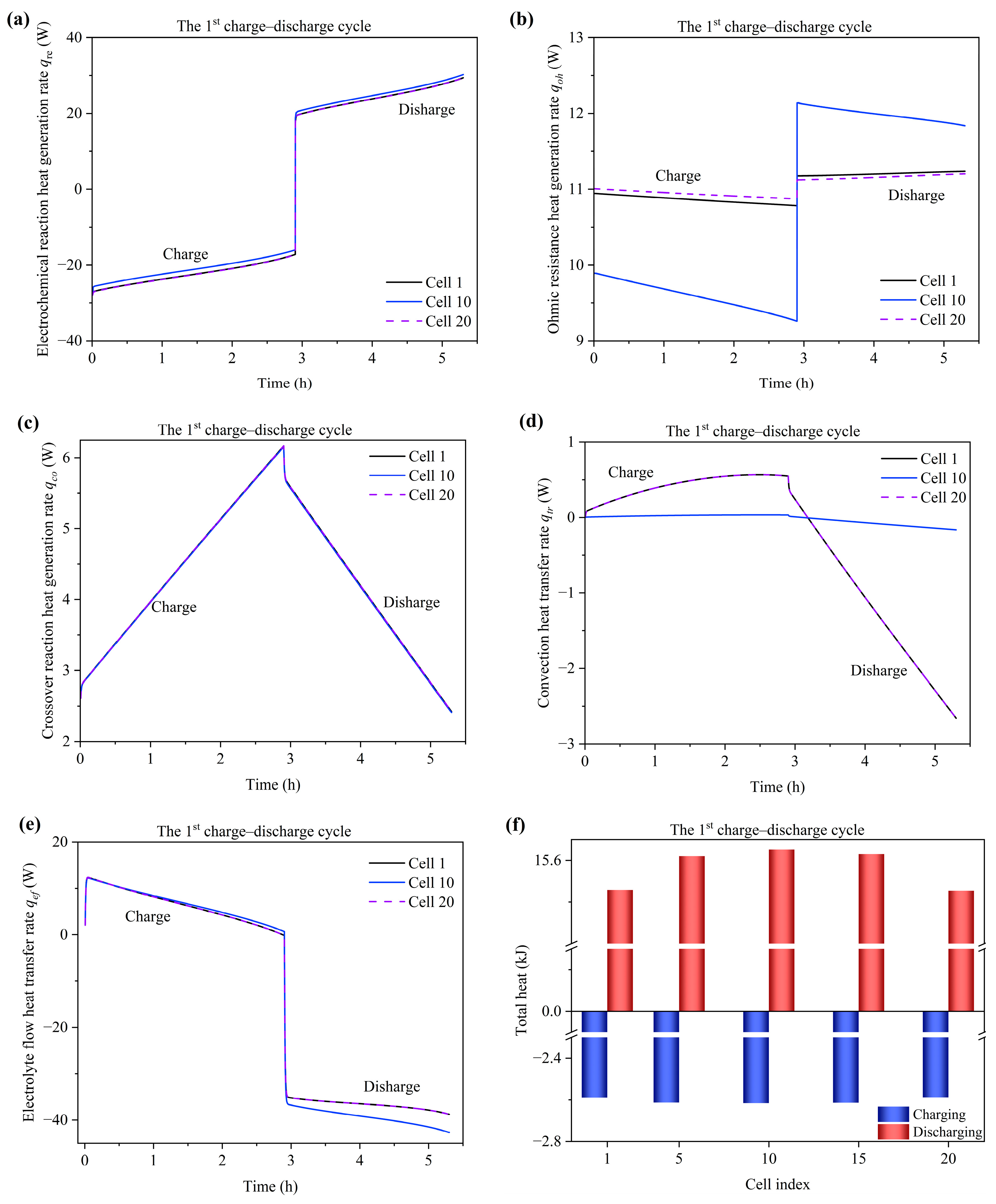
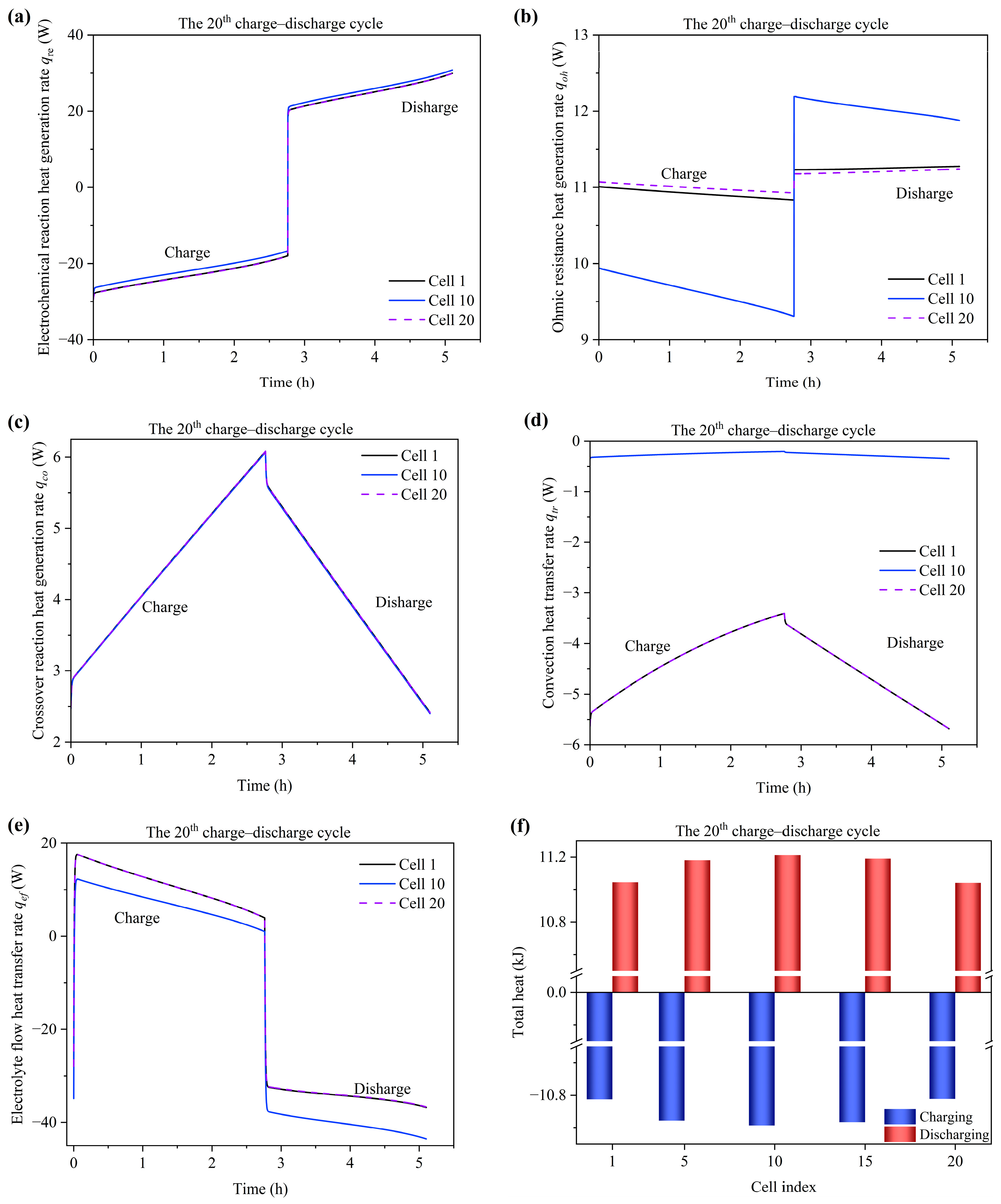
• At the alternating point between the charge and discharge process, the temperature variation of the tank is hysteretic when compared with the stack. Moreover, the temperature of the end cells (1st and 20th cells) experiences a sharper decrease compared to the middle cells due to the large degree of heat dissipation from the endplate to the environment. The temperature of the stack is mainly influenced by the electrochemical reaction and electrolyte flow heat transfer between the cell and tank. Heat generation from the ohmic resistance is an intermediate influencing factor. Heat generation from the crossover reaction and convection heat transfer between the cell and environment are the least impactful factors.
• The temperature of the stack will exceed 40 °C during the charge–discharge cycles when operating at 60 A and an ambient temperature of 30 °C. To keep the stack temperature below 40 °C, a new tank cooling strategy is proposed and saves 27.18% of the air conditioning energy consumption during 20 charge–discharge cycles.

References

1. Shi, X.; Zheng, Y.; Lei, Y.; Xue, W.; Yan, G.; Liu, X.; Cai, B.; Tong, D.; Wang, J. Air quality benefits of achieving carbon neutrality in China. Sci. Total Environ. 2021, 795, 148784. [Google Scholar] [CrossRef] [PubMed]
2. Jiao, Y.-H.; Zhang, Z.-K.; Dou, P.-Y.; Xu, Q.; Yang, W.-W. Consistency analysis and resistance network design for vanadium redox flow battery stacks with a cell-resolved stack model. Int. J. Green Energy 2023, 20, 166–180. [Google Scholar] [CrossRef]
3. Ren, J.; Wei, L.; Wang, Z.; Yue, Q.; Liu, B.; Jia, G.; Fan, X.; Zhao, T. An electrochemical-thermal coupled model for aqueous redox flow batteries. Int. J. Heat Mass Transf. 2022, 192, 122926. [Google Scholar] [CrossRef]
4. Kazacos, M.; Cheng, M.; Skyllas-Kazacos, M. Vanadium redox cell electrolyte optimization studies. J. Appl. Electrochem. 1990, 20, 463–467. [Google Scholar] [CrossRef]
5. Trovò, A.; Guarnieri, M. Standby thermal management system for a kW-class vanadium redox flow battery. Energy Convers. Manag. 2020, 226, 113510. [Google Scholar] [CrossRef]
6. Skyllas-Kazacos, M.; McCann, J.; Li, Y.; Bao, J.; Tang, A. The Mechanism and Modelling of Shunt Current in the Vanadium Redox Flow Battery. ChemistrySelect 2016, 1, 2249–2256. [Google Scholar] [CrossRef]
7. Wandschneider, F.T.; Röhm, S.; Fischer, P.; Pinkwart, K.; Tübke, J.; Nirschl, H. A multi-stack simulation of shunt currents in vanadium redox flow batteries. J. Power Sources 2014, 261, 64–74. [Google Scholar] [CrossRef]
8. Al-Fetlawi, H.; Shah, A.A.; Walsh, F.C. Non-isothermal modelling of the all-vanadium redox flow battery. Electrochim. Acta 2009, 55, 78–89. [Google Scholar] [CrossRef]
9. Tang, A.; Ting, S.; Bao, J.; Skyllas-Kazacos, M. Thermal modelling and simulation of the all-vanadium redox flow battery. J. Power Sources 2012, 203, 165–176. [Google Scholar] [CrossRef]
10. Tang, A.; Bao, J.; Skyllas-Kazacos, M. Thermal modelling of battery configuration and self-discharge reactions in vanadium redox flow battery. J. Power Sources 2012, 216, 489–501. [Google Scholar] [CrossRef]
11. Wei, Z.; Zhao, J.; Skyllas-Kazacos, M.; Xiong, B. Dynamic thermal-hydraulic modeling and stack flow pattern analysis for all-vanadium redox flow battery. J. Power Sources 2014, 260, 89–99. [Google Scholar] [CrossRef]
12. Trovò, A.; Saccardo, A.; Giomo, M.; Guarnieri, M. Thermal modeling of industrial-scale vanadium redox flow batteries in high-current operations. J. Power Sources 2019, 424, 204–214. [Google Scholar] [CrossRef]
13. Kirk, E.H.; Fenini, F.; Oreiro, S.N.; Bentien, A. Temperature-Induced Precipitation of V2O5 in Vanadium Flow Batteries—Revisited. Batteries 2021, 7, 87. [Google Scholar] [CrossRef]
14. Han, S.; Tan, L. Thermal and efficiency improvements of all vanadium redox flow battery with novel main-side-tank system and slow pump shutdown. J. Energy Storage 2020, 28, 101274. [Google Scholar] [CrossRef]
15. Wang, H.; Soong, W.L.; Pourmousavi, S.A.; Zhang, X.; Ertugrul, N.; Xiong, B. Thermal dynamics assessment of vanadium redox flow batteries and thermal management by active temperature control. J. Power Sources 2023, 570, 233027. [Google Scholar] [CrossRef]
16. Yan, Y.; Li, Y.; Skyllas-Kazacos, M.; Bao, J. Modelling and simulation of thermal behaviour of vanadium redox flow battery. J. Power Sources 2016, 322, 116–128. [Google Scholar] [CrossRef]
17. Tang, A.; McCann, J.; Bao, J.; Skyllas-Kazacos, M. Investigation of the effect of shunt current on battery efficiency and stack temperature in vanadium redox flow battery. J. Power Sources 2013, 242, 349–356. [Google Scholar] [CrossRef]
18. Zhang, Y.; Zhao, J.; Wang, P.; Skyllas-Kazacos, M.; Xiong, B.; Badrinarayanan, R. A comprehensive equivalent circuit model of all-vanadium redox flow battery for power system analysis. J. Power Sources 2015, 290, 14–24. [Google Scholar] [CrossRef]
19. Ye, Q.; Hu, J.; Cheng, P.; Ma, Z. Design trade-offs among shunt current, pumping loss and compactness in the piping system of a multi-stack vanadium flow battery. J. Power Sources 2015, 296, 352–364. [Google Scholar] [CrossRef]
20. Trovò, A.; Picano, F.; Guarnieri, M. Comparison of energy losses in a 9 kW vanadium redox flow battery. J. Power Sources 2019, 440, 227144. [Google Scholar] [CrossRef]
21. Xiao, W.; Tan, L. Control strategy optimization of electrolyte flow rate for all vanadium redox flow battery with consideration of pump. Renew. Energy 2019, 133, 1445–1454. [Google Scholar] [CrossRef]
22. Tang, A.; Bao, J.; Skyllas-Kazacos, M. Studies on pressure losses and flow rate optimization in vanadium redox flow battery. J. Power Sources 2014, 248, 154–162. [Google Scholar] [CrossRef]
23. Jirabovornwisut, T.; Kheawhom, S.; Chen, Y.-S.; Arpornwichanop, A. Optimal operational strategy for a vanadium redox flow battery. Comput. Chem. Eng. 2020, 136, 106805. [Google Scholar] [CrossRef]
24. Kim, D.K.; Yoon, S.J.; Lee, J.; Kim, S. Parametric study and flow rate optimization of all-vanadium redox flow batteries. Appl. Energy 2018, 228, 891–901. [Google Scholar] [CrossRef]
25. Shah, A.A.; Tangirala, R.; Singh, R.; Wills, R.G.A.; Walsh, F.C. A Dynamic Unit Cell Model for the All-Vanadium Flow Battery. J. Electrochem. Soc. 2011, 158, A671. [Google Scholar] [CrossRef]
26. Yue, M.; Lv, Z.; Zheng, Q.; Li, X.; Zhang, H. Battery assembly optimization: Tailoring the electrode compression ratio based on the polarization analysis in vanadium flow batteries. Appl. Energy 2019, 235, 495–508. [Google Scholar] [CrossRef]
27. Wang, Q.; Qu, Z.G.; Jiang, Z.Y.; Yang, W.W. Experimental study on the performance of a vanadium redox flow battery with non-uniformly compressed carbon felt electrode. Appl. Energy 2018, 213, 293–305. [Google Scholar] [CrossRef]
28. Hietaharju, P.; Ruusunen, M.; Leiviskä, K. A Dynamic Model for Indoor Temperature Prediction in Buildings. Energies 2018, 11, 1477. [Google Scholar] [CrossRef]
29. Kim, N.-K.; Shim, M.-H.; Won, D. Building Energy Management Strategy Using an HVAC System and Energy Storage System. Energies 2018, 11, 2690. [Google Scholar] [CrossRef]
Figure 1. Hydraulic resistance network model of electrolyte flow in VRFB stack.
Batteries 10 00347 g001
Figure 2. The equivalent circuit model considering the shunt currents of the VRFB stack.
Batteries 10 00347 g002
Figure 3. Model validation by comparing battery voltage (a) and temperature (b) of present model and experimental data from the reference [3].
Batteries 10 00347 g003
Figure 4. Flow rate deviation of cells in stack.
Batteries 10 00347 g004
Figure 5. Shunt currents in manifolds (a) and channels (b) across single cells, current of single cells at end of charging (c) and discharging (d), and cell current variation during charging (e) and discharging (f). All current data are obtained at current of 60 A in 20th charge–discharge cycle.
Batteries 10 00347 g005
Figure 6. Single-cell voltage variation during charging and discharging of 20th charge–discharge cycle (a); single-cell voltage distribution at end of charging and discharging of 20th charge–discharge cycle (b).
Batteries 10 00347 g006
Figure 7. The electrolyte temperature variation of the center cell, outlet pipe, tank and inlet pipe during 20 charge–discharge cycles. The charge and discharge currents are 60 A.
Batteries 10 00347 g007
Figure 8. In the 20th charge–discharge cycle, the electrolyte temperature variation of the center cell, outlet pipe, tank and inlet pipe is shown. The charge and discharge currents are 60 A.
Batteries 10 00347 g008
Figure 9. Cell temperature variation in the 1st charge–discharge cycle (a); the cell temperature distribution at the end of charging and discharging of the 1st charge–discharge cycle (b). Cell temperature variation in the 20th charge–discharge cycle (c); the cell temperature distribution at the end of charging and discharging of the 20th charge–discharge cycle (d). The charge and discharge currents are 60 A.
Batteries 10 00347 g009
Figure 10. The heat generation rate of the electrochemical reaction (a), ohmic resistance (b) and crossover reaction (c); the heat transfer rate of convection between the cell and environment (d); the heat transfer rate of the electrolyte flow between the cell and pipe (e); the total heat variation of single cells, where positive and negative values denote the temperature increment and decrement of single cells, respectively (f). All of the data are derived from the 1st charge–discharge cycle at a current of 60 A.
Batteries 10 00347 g010
Figure 11. The heat generation rate of the electrochemical reaction (a), ohmic resistance (b) and crossover reaction (c); the heat transfer rate of convection between the cell and environment (d); the heat transfer rate of the electrolyte flow between the cell and pipe (e); the total heat variation of single cells, where positive and negative values denote the temperature increment and decrement of single cells, respectively (f). All of the data are derived from the 20th charge–discharge cycle at a current of 60 A.
Batteries 10 00347 g011
Figure 12. The heat transfer rate of the stack, pipe and tank (a); the total heat transfer (b) of the 20th charge–discharge cycle. The ambient temperature is 25 °C, and the charge and discharge currents are 60 A.
Batteries 10 00347 g012
Figure 13. The temperature variation of the stack at different ambient temperatures (a); the equilibrium temperatures of stack variation with ambient temperatures (b). The charge and discharge currents are 60 A.
Batteries 10 00347 g013
Figure 14. The stack temperature variation without and with the common room cooling control strategy, and the room temperature is controlled at 26.9 °C (a) and 26.7 °C (b). The ambient temperature is 30 °C, and the charge and discharge currents are 60 A.
Batteries 10 00347 g014
Figure 15. The stack temperature variation without and with the new tank cooling control strategy, and the room temperature is controlled at 26.7 °C (a) and 26.3 °C (b). The ambient temperature is 30 °C, and the charge and discharge currents are 60 A.
Batteries 10 00347 g015
Figure 16. The power (a) and energy consumption (b) of the air conditioning with the new tank cooling control strategy and the common room cooling control strategy. The ambient temperature is 30 °C, and the charge and discharge currents are 60 A.
Batteries 10 00347 g016