Linear Regression-Based Procedures for Extraction of Li-Ion Battery Equivalent Circuit Model Parameters

Abstract

Equivalent circuit models represent one of the most efficient virtual representations of battery systems, with numerous applications supporting the design of electric vehicles, such as powertrain evaluation, power electronics development, and model-based state estimation. Due to their popularity, their parameter extraction and model parametrization procedures present high interest within the research community, with novel approaches at an elementary level still being identified. This article introduces and compares in detail two novel parameter extraction methods based on the distinct application of least squares linear regression in relation to the autoregressive exogenous as well as the state-space equations of the double polarization equivalent circuit model in an iterative optimization-type manner. Following their application using experimental data obtained from an NCA Sony VTC6 cell, the results are benchmarked against a method employing differential evolution. The results indicate the least squares linear regression applied to the state-space format of the model as the best overall solution, providing excellent accuracy similar to the results of differential evolution, but averaging only 1.32% of the computational cost. In contrast, the same linear solver applied to the autoregressive exogenous format proves complementary characteristics by being the fastest process but presenting a penalty over the accuracy of the results.

1. Introduction

1.1. Motivation and Challenges

Electric and hybrid electric vehicles, since they offer an affordable, more efficient, and potentially sustainable form of propulsion compared to conventional internal combustion vehicles, are receiving an increasing amount of attention from the research community. One of the defining elements of one vehicle is considered the battery system, as its development, manufacturing, and operation have significant implications over the lifespan of the vehicle, as well as its disposal and recycling. Consequently, research and development of elements contributing at each stage of the product cycle receive considerable attention as they have the potential to reduce cost while enhancing the performance and lifespan of the battery system.

One such element is represented by simulation models, which can range from simplistic static data-driven representations to complex multiscale and multidimensional internal representations of the electrochemical cell. Due to its attractive balance between the resources required to develop and the capability to replicate the battery system voltage response with sufficient accuracy, one of the most popular options is presented by equivalent circuit models (ECMs). These play a significant role during the development cycle, with applications such as simulating the battery using Hardware-in-the-Loop systems, powertrain evaluation, as well as the development of power electronics such as the battery management system (BMS). Contributions from this model are also present in the live management of the battery during vehicle operation, as model-based state estimation within the BMS is used to complete a series of functions, with the most popular being the estimation for the State of Charge (SOC).

1.2. Literature Review

Accurate parametrization represents one of the most important prerequisites for a model to be effective in any application, placing the extraction of parameter values from data as well as the structure of parameters under attention. In relation to ECMs, numerous methodologies are already available in specialized literature and cover a wide array of use cases. Summaries proposed by Kalogiannis et al. [1] and Li et al. [2] indicate the main techniques used in relation to time-domain data to be based on least squares linear regression (LS), Kalman filters (KF), generic optimizers, and analytical equations applied to step responses. If the model is parametrized in the frequency domain, electrochemical impedance spectroscopy is commonly employed to directly obtain the parameter values.

The essential parametrization procedures employing least squares linear regression are founded on the property of the ECM being a linear dynamic model. This implies the model can be formulated as a discrete transfer function and implicitly as an autoregressive exogenous model (ARX). This procedure is well covered by system identification theory, as highlighted by sources such as Ljung, L. [3], while in relation to battery ECMs, an exemplification of the simple procedure is presented by Zhang et al. [4]. More advanced studies, such as the one presented by Huang, C.-S. [5], target the improvement of the results obtained by this procedure from one data sample by considering characteristics such as the load profile, gradient of Open Circuit Voltage with respect to SOC, and condition number in the segmentation process of the data.

A more commonly employed extension of least squares applied to the ARX model procedure is presented by recursive least squares (RLS). The recursive part refers to a secondary component to the aforementioned procedure which recomputes the results and updates parameter values recursively. A plain exemplification of the process is presented by Raihan et al. [6], while most recent studies targeting this type of procedure attempt to increase the accuracy and robustness of the methodology through newly added elements. These include condition numbers as presented by Kim et al. [7], single or multiple forgetting factors, as suggested by Fan et al. [8] and Xia et al. [9], adapting forgetting factors, as exemplified by Sun, X. et al. [10], and computation over one specific window length (fixed memory), as demonstrated in the study by Sun, C. et al. [11]. In line with the fact that RLS-based studies generally discuss and target online applications, these benefit substantially live parameter estimation methodologies, as they increase the flexibility and ability of the procedure to track more accurately the change in parameters. However, the additions also present a series of downsides, such as the additional computational power as well as expertise and engineering effort to set up correctly. The latter is further highlighted by the proposed procedure by Xia et al. [9] containing Particle Swarm Optimization to determine the optimal forgetting factors added to an RLS process. Nevertheless, as most studies target to improve the iterative update procedure and not the essential least squares linear regression component, in the case of offline procedures, the existing research fails to bring significant advantages. This results from the complete dataset being readily available, allowing for the results to be considered in other manners such as collectively rather than iteratively, meaning the tracking ability may not be necessary.

The same issue is shared by the group of procedures based on Kalman filters or similar methodologies as they present a highly similar probability inference mechanism intended for supporting the tracking of the identified parameter values. The additional computational and engineering effort required to effectively set this part of the process will often render this type of option uncommon. This is supported by a close examination of the work presented by Li et al. [12] targeting to use this procedure to track only the slow dynamics of the system and the similar particle filter-based approach proposed by Xu et al. [13]. The Kalman filter-based procedures present as a common process used in relation to battery ECMs but represent an unpopular option for model parametrization. Instead, as exemplified by Fan et al. [8], Xia et al. [9], or Sun, C. et al. [11], they present a common option for SOC estimation tasks.

Outside the popular extension from linear regression to RLS, two other subgroups target the application of the least squares regression procedure directly to the state-space format of model equations and present interest for offline applications. Since the ECM presents as a linear dynamic model, the response to a step input can be summarized as a simple exponential function whose partial derivatives with respect to each model parameter can be easily computed. Consequently, a curve-fitting approach employing nonlinear least squares regression (NLS) becomes feasible, iteratively reducing error by using the local linearization of the objective function with respect to the targeted parameters. This type of approach is exemplified by Tian et al. [14], while an alternative implementation of NLS is also presented by Tran et al. [15] by directly employing the nlinfit function of MATLAB. The alternative implementation replaces the analytical computation of the derivatives with multiple evaluations of the objective function, becoming applicable outside step response data— at the cost, however, of computational effort. A completely different approach, limited also to step response, is represented by work presented by Chen, C. [16], which, through repeated integration and regrouping of parameters, obtains a new set of linear parameters to be directly identified by applying linear regression.

Another group of options is presented by the procedures based on predefined optimization packages. Following their flexibility, ease of implementation, and accuracy, these represent one of the most popular state-of-the-art options in recent published studies. Exemplifications are presented by Al Rafei et al. [17] proposing the ECM parametrization using the Genetic Algorithm complemented by the Taguchi Method, while Zhou et al. [18] introduce a hybrid coupling between particle swarm optimization and simulated annealing for the same task. Hybridization of the procedure towards the benefit of computational efficiency and accuracy can also be achieved in series, as presented by Ghoulam et al. [19], by employing, in sequence, the Fminsearch, Fmincon, and Genetic Algorithm found as readily available within the MatLab Optimization Toolbox. More comprehensive investigations, such as the ones proposed by Cheng, Y. S. [20] and Hou et al. [21], also present comparisons between multiple optimization algorithms in relation to the ECM parametrization problem.

Nevertheless, the benefits of the optimization-based procedures are also severely offset by their very high computational demand. This is directly associated with the number of degrees of freedom present in the optimization (number of parameters) as well as the absence of information over the optimization task other than the repeated evaluations of the objective function. While existent research may attempt to indicate one type of optimization to converge faster than another, the comparisons are highly dependent on multiple factors such as the data employed, model structure, and initialization, and cannot be used as a guarantee against a differently defined use case. At the same time, research attempting to add more information over the optimization task from a more effective source could present a more significant and permanent advantage in computational effort.

The last main group of procedures suitable for ECM parametrization support the analytical extraction from step response data, with examples such as the ones presented by Lee, S. et al. [22]. While highly effective, this type of procedure presents as the most rudimentary and is advised only for one-time procedures. The recommendation follows their easy implementation at the expense of human assistance and the use of a limited amount of information captured in a step response in the absence of multiple repetitions.

Machine learning techniques were also considered of interest for battery modeling. These have been used previously for a different category of models, capturing the complex relations between various factors and the state of the system empirically. Exemplification for this type of approach is presented by the study proposed by Lee, J. et al. [23], targeting the prediction of remaining useful life using artificial neural networks. By comparison, the effective extraction of ECM parameters from an individual segment of data represents a significantly different task. The ECM is a useful and simple algorithmic representation of the battery in its current state, which can be calibrated very effectively using the procedure detailed here. However, modeling the complex variation in ECM parameters as a function of the battery system state (e.g., SOC, SOH) may be a beneficial application of machine learning complementing the proposed novel procedures.

1.3. Main Contribution

This work sets to introduce, describe, and analyze in detail two novel methodologies, representing the main research contribution of the paper. These present the capability of effectively extracting ECM parameters from individual samples of battery voltage response data and are based on least squares linear regression (commonly referred to as ordinary least squares and abbreviated as LS throughout this work).

The first procedure is based on the well-known transformation to the ARX format, where the proposed improvement is the repetition of the process as part of a fully automated and consistent optimization of the data preprocessing parameters. This addition targets directly a reduction in MSE for the LS-based identification of parameter values. The second procedure applies the same linear solver to both linear and nonlinear parameters of the state-space format equations of the model. For this second option, the research contribution is presented by the new two-step procedure structure and the methodology for computing the local linearization for the nonlinear parameters. These enable the effective application of LS towards the extraction of ECM parameter values from any type of data. Finally, a procedure based on a global optimizer, namely differential evolution, is detailed, without any direct research contribution, but with the main goal to provide an accuracy benchmark for the results, following an endorsement of accuracy in previous research for optimization-based procedures. The additional comparison against a global optimizer is also set to highlight the methods strengths and weaknesses as well as provide a better understanding of the suitability of each method in relation to any application.

By contrast with the existing published research, the first procedure proposed attempts to improve the accuracy of the LS component applied to the ARX format found within system identification theory as well as part of the RLS procedures by integrating an additional optimization adjusting the preprocessing of the data. At the same time, the second procedure represents an updated version of multiple groups summarized in this section. By comparison with the LS-ARX procedures, however, it can apply the LS straight to the state-space format without being limited to step response data. This limitation is presented by some of the NLS procedures or procedures employing integration. The effective integration of gradient information and LS also leads to a large reduction in computational effort, with no penalty over accuracy, in comparison to optimization-based procedures. The procedure can also be considered a case of nested linear/nonlinear optimization. The example presented by Cleary et al. [24] represents a procedure with the most similar structure to date relative to the second procedure proposed in this study. Nevertheless, the novel proposed method in this study has the capability of using linear regression for both groups of parameters. The consequence is presented by a substantial computational advantage, while the prior published work uses particle swarm optimization for the nonlinear part, stating the use of linear regression for this task as an impossibility.

1.4. Article Organization

The remaining part of the paper is structured as follows: Section 2 introduces the model structure, mathematical foundations and methodologies of both parametrization procedures, as well as the methodology employed for the acquisition of experimental data. Section 3 contains an overview of the results, targeting an overview of the accuracy and efficiency of each procedure. Section 4 contains a detailed analysis of each new parametrization procedure proposed, while Section 5 follows with concluding remarks.

2. Materials and Methods

2.1. Model Structure

The equivalent circuit model structure, commonly referred to as the 2RC or ‘double polarization’ model, illustrated in Figure 1, has been selected to demonstrate all 3 parametrization procedures. The selection for the second order was based on popularity as well as a compromise between accuracy and complexity, as none of the 3 processes presents any limitation towards a different order of the RC model. The generic continuous state-space model has been summarized in two main equations rearranged according to the state-space format. Equation (1) resulted from directly applying Kirchhoff’s second law to the main circuit loop. Equation (2) was obtained by employing both the first and second law of Kirchhoff for the RC element loops together with a definition of capacitive current; its derivation can be found in Appendix A.

$$V_{Out}(t)=V_{OC}-\sum _{i=1}^n{R}_i{I}_i\left(t\right)-R_0{I}_0(t)$$

(1)

$${\displaystyle \frac{d{I}_i(t)}{dt}}={\displaystyle \frac{-1}{{\tau }_i}}{I}_i(t)+{\displaystyle \frac{1}{{\tau }_i}}{I}_0(t)$$

(2)

where ${\tau }_i=R_i{C}_i$ represents the parameters associated with RC element number $i$, $n$ is the order of the RC model, $I_i$ is the current associated with each RC element, $R_0$ is the series resistance, $I_0$ the input current, and $V_{Out}$ is the voltage response of the model. To achieve discretization of the model, the forwards Euler method presented by Zeigler, B. [25] was employed. The process turned Equation (2) into Equation (3), following the derivation captured in Appendix B, while Equation (1) does not require any changes.

$$I_i\left(t_{k+1}\right)=\left(1-{\displaystyle \frac{∆t}{{\tau }_i}}\right)I_i\left(t_k\right)+{\displaystyle \frac{∆t}{{\tau }_i}}{I}_0(t_k)$$

(3)

where $t_k$ is the time in seconds at time step $k$ and $∆t=t_{k+1}-t_k$.

To obtain the ARX format of the model captured by Equations (1) and (3), the z-transform process presented by Cheever, E. [26] is applied to both model equations. The result is then used to conduct the conversion from state-space form to a discrete transfer function, also documented by Cheever, E. [27]. The resulting model, having a constant term ($c$) to account for the Open Circuit Voltage parameter, is captured in Equation (4). The complete process described in this paragraph can be found in Appendix C. The equations defining the relations between ARX and state-space formats have also been summarized in

Table 1. ARX-state-space parameters mapping equations.

ARX Parameter	Equation
$a_1$	${\displaystyle \frac{∆t}{{\tau }_2}}+{\displaystyle \frac{∆t}{{\tau }_1}}-2$
$a_2$	${\displaystyle \frac{{∆t}^2}{{\tau }_1{\tau }_2}}-{\displaystyle \frac{∆t}{{\tau }_1}}-{\displaystyle \frac{∆t}{{\tau }_2}}+1$
$b_0$	$R_0$
$b_1$	${\displaystyle \frac{R_0∆t}{{\tau }_1}}+{\displaystyle \frac{R_0∆t}{{\tau }_2}}+{\displaystyle \frac{R_1∆t}{{\tau }_1}}+{\displaystyle \frac{R_2∆t}{{\tau }_2}}-2R_0$
$b_2$	${\displaystyle \frac{R_0{∆t}^2}{{\tau }_1{\tau }_2}}+{\displaystyle \frac{R_1∆t^2}{{\tau }_1{\tau }_2}}+{\displaystyle \frac{R_2{∆t}^2}{{\tau }_1{\tau }_2}}-{\displaystyle \frac{R_0∆t}{{\tau }_1}}-{\displaystyle \frac{R_0∆t}{{\tau }_2}}-{\displaystyle \frac{R_1∆t}{{\tau }_1}}-{\displaystyle \frac{R_2∆t}{{\tau }_2}}+R_0$
$c_{min/max}$	$\left(1+a1+a2\right)\times V_{OC,min/max}$

for the 2RC order model.

$$V_{Out}\left(z\right)=c-\sum _{i=1}^n{a}_i{V}_{Out}{z}^{-i}-\sum _{i=0}^n{b}_i{I}_0{z}^{-i}$$

(4)

The study presented will only target individual segments of the experimental data. These have been assumed to present insignificant variation for parameter values caused by changes in operating conditions, namely SOC and temperature. Consequently, the parameters are assumed to maintain constant values throughout each segment of data, meaning only one locally correct value for each parameter to be identified. Modeling additional nonlinear dependence against temperature, SOC, or current amplitude for the parameter values is out of the scope of the work presented but represents the aim of future publications. Nevertheless, the assumption of one value being sufficient for each segment of data requires one exception for the Open Circuit Voltage ($V_{OC}$) parameter due to its significant variation relative to SOC. Consequently, two values are identified for each segment of data, associated with the minimum and maximum SOC values within each data sample. By assuming a local linear relation between the $V_{OC}$ and SOC for the short SOC range covered by each data segment, the value at each time point is the result of linear interpolation between the two values. The change transforms Equations (1) and (4) into Equations (5) and (6), while the linear interpolation between the two distinct values is described by Equation (7). The exception is designed to enable the LS process to correctly attribute part of the dynamic behaviour to Open Circuit Voltage variation, which becomes significant, especially during long discharge pulses.

$$V_{Out}\left(t_{k+1}\right)=\left(V_{OC,max}\times p_{SOC}(t_k)+V_{OC,min}\times (1-p_{SOC}(t_k))\right)-R_0{I}_0(t_k)-\sum _{i=1}^n{R}_i{I}_i(t_k)$$

(5)

$$V_{Out}\left(z\right)=\left(c_{OCV,max}\times p_{SOC}(t_k)+c_{OCV,min}\times {(1-p}_{SOC}(t_k))\right)-\sum _{i=1}^n{a}_i{V}_{Out}{z}^{-i}-\sum _{i=0}^n{b}_i{I}_0{z}^{-i}$$

(6)

$$p_{SOC}(t_k)={\displaystyle \frac{SOC\left(t_k\right)-{SOC}_{min}}{{SOC}_{max}-{SOC}_{min}}}$$

(7)

2.2. Parameter Extraction Procedures

The three proposed parameter extraction methods introduced are demonstrated using step response sections of data. Nevertheless, the mathematical underpinnings of all three allow extraction of parameters from any ad hoc measurements produced using an arbitrary current input to the battery system since both procedures do not include any assumption over the shape of the input current or voltage response.

The only assumption integrated targets the initial condition of the model, as the current through the resistance associated with each RC element is set to 0 at $k=1$. This was considered reasonable as the cell was at the end of a long rest period before the current pulse was applied. The data employed were obtained from a Sony VTC6 and are part of a larger dataset acquired using the methodology described in Section 2.3. For direct comparison, the evaluation of results presented by the three procedures employed the same mean squared error (MSE) objective function described by Equation (8).

$$MSE={\displaystyle \frac{1}{m}}\sum _{k=1}^m{\left(V_{Exp}(t_k)-V_{Out}(t_k)\right)}^2$$

(8)

where $m$ is the number of time steps in the data sample, $V_{Exp}$ is the experiment-measured voltage, and $V_{Out}$ is the model response.

The objective for all three procedures is set to minimize the squared error between the model response and ad hoc time-domain experimental data. As a result, in the absence of further proof, the results should be considered an empirical fit over the data, and not one aligned with the physical attributes of the system capable of rendering a correct phenological/physical model. This observation carries importance, especially in the case of ad hoc data segments which may not capture sufficiently phenomena associated with the actual physical system. However, these can be used and replicated empirically by the ECM, with one of the most common examples being represented by drive cycle data.

2.2.1. Parameter Extraction Using the ARX Model Format and Least Squares Linear Regression (LS-ARX)

Following the description of linear dynamic systems using discrete transfer functions, rearranging the terms of the equation will result in what is commonly referred to as an autoregressive exogenous model (ARX). The identification of the model is well established in system identification theory and is achieved by employing LS, as demonstrated by Ljung, L. in his summary [3] and described in (9), which can also be solved by a linear solver. Once the ARX format parameters have been found, reversing the z-transform using the equations summarized in Table 1 will result in the state-space format parameter values.

$$\gamma =({A^{T}A)}^{-1}{A}^{T}B$$

(9)

where $A,B$ are the design and response matrices for a data sample, with m time steps used to extract the parameters for the nth order of the model contained by matrix $\gamma$, as expanded below.

$$\gamma ={\left[\begin{array}{cccccccc}{c}_{OCV,max}& c_{OCV,min}& a_1& \cdots & a_n& b_0& \cdots & b_n\end{array}\right]}^T$$

$$A=\left[\begin{array}{cccccccc}{p}_{soc}\left(t_{n+1}\right)& 1-p_{soc}{(t}_{n+1})& V_{Exp}\left(t_n\right)& \cdots & V_{Exp}\left(t_1\right)& I_0\left(t_{n+1}\right)& \cdots & I_0\left(t_1\right)\\ p_{soc}\left(t_{n+2}\right)& 1-p_{soc}\left(t_{n+2}\right)& V_{Exp}\left(t_{n+1}\right)& \cdots & V_{Exp}\left(t_2\right)& I_0\left(t_{n+2}\right)& \cdots & I_0\left(t_2\right)\\ & & \ddots & & \ddots & \ddots & \ddots \\ p_{soc}\left(t_m\right)& {1-p}_{soc}\left(t_m\right)& V_{Exp}\left(t_{m-1}\right)& \cdots & V_{Exp}\left(t_{m-n}\right)& I_0\left(t_m\right)& \cdots & I_0\left(t_{m-n}\right)\end{array}\right]$$

$$B=\left[\begin{array}{c}{V}_{Exp}\left(t_{n+1}\right)\\ V_{Exp}\left(t_{n+2}\right)\\ \ddots \\ V_{Exp}\left(t_m\right)\end{array}\right]$$

By considering the application of LS in the identification of ARX parameters from individual data segments, the significant effect of two factors has been described below, while also being supported by the results and discussion in Section 4.1.

Factor 1—conditioning of least squares linear regression. This factor reflects the variance of the LS result and is directly correlated with the observability of the parameters from the data provided as well as other mathematical concepts such as the covariance matrix and condition number. Examples of studies considering this factor are scarce and include studies such as the one presented by Kim et al. [7], which uses the condition number to set the forgetting factor in a recursive approach. A separate example is also provided by Huang, C.-S. [5], which uses multiple criteria to efficiently devise data samples. As a result, well-conditioning of the LS is rarely considered, despite having a significant impact on the results. The factors which can directly influence this are numerous, with the most common being the number of parameters to be identified (resulting from the order of the RC model selected and directly influencing the sensitivity of the model response relative to the parameters), the sampling of the data (high sample rates will reduce the fraction of the response captured by each time step), maneuvers captured by the data (lack of information), and behavior of the system (observability of individual phenomena in time-domain data). While improving the conditioning will likely result in more accurate results when applying LS, the true objective of the procedure to be presented is represented by the reduction in error between the experimental data and the simulated result. Consequently, if an additional process is set in support of the LS process, it should target directly the minimization of error rather than another indicator as the main objective. In the list of factors affecting the conditioning, the sampling rate and order of the model are the only controllable items when considering data which has already been acquired. Consequently, they are also the only ones that could be potentially optimized towards supporting a more accurate result.

Factor 2—error propagation. Noise is not considered a significant issue when considering the capability of LS to provide unbiased results for a problem. Nevertheless, when considering the application in relation to the ARX model, it can be observed that the voltage response values are captured not only by the response matrix but also by the design matrix of the regression. Consequently, the measurement noise associated with it will affect not only the dependent values of the regression but also the independent ones. This leads to a case of error-in-variables, which, in the case of simple LS, is set to cause a biased result, sometimes referred to as attenuation bias. This will cause an error margin correlated with the noise levels found within the experimental data.

The investigation presented in this paper will target to reduce the negative impact of the aforementioned issues associated with LS being applied to the ARX format model. By adding two additional degrees of freedom to the process, a direct reduction in error between the resulting model response and experimental data can be achieved. The degrees of freedom will control parameters used in the preprocessing of each data segment, namely the size of a moving average filter window as well as the sampling period, by introducing downsampling. Manually adjusting the same parameters may also represent an effective process in the case of a small number of data segments being processed by an experienced engineer. However, this option was not deemed a feasible approach in the case of large datasets or when automation of the process over multiple arbitrary datasets (e.g., experiment, real driving cycles) is desirable. Consequently, an automated search procedure is proposed to complement the extraction of the ARX parameters using LS to the benefit of both online and offline procedures.

The complete process is illustrated in Figure 2. The starting point is presented by the MSE value obtained for one data sample without conducting any preprocessing of the experimental data. This sets a benchmark result, which is then compared and potentially replaced with other results after the same data has been filtered using a moving average (MA) filter and sampled down to a lower data point frequency.

The control is achieved by 4 distinct values: 2 memorizing the current values and 2 memorizing the next values to be assessed for the filter window size (FWS) and the sampling period (SP) of the data. At the beginning of the process, the current FWS and sampling period are set to 1 and the default equidistant SP of the data, while the next values are set to 4 and double the value of the default SP. At each iteration, the algorithm will try to obtain a better result by using the next FWS value and the current value for the SP. If this results in a lower mean squared error (MSE), the next value becomes the current one, and the next FWS is multiplied by 2. However, if unsuccessful, downsampling the data by a higher factor is tried, hence using the current value for the FWS and the next value for the SP, followed by the same MSE test. This decides whether to set the current SP to the value of the next SP and multiply the latter by 2. If both attempts fail to bring an improvement, a failed iteration is counted and both next values are multiplied by 4, targeting the acceleration of the algorithm and potential avoidance of a local minimum. The algorithm allows for a maximum of 3 failed iterations, then stops and outputs the parameter values associated with the lowest mean squared error. The final result is represented by an optimization-type approach complementing the identification of ARX parameters using linear regression, a process which has not been previously presented in published research.

The additional process described in support of least squares linear regression can also be interpreted as a search algorithm for the two-parameter values associated with the local minimum of the MSE via an iterative approach. This observation carries importance, as it also highlights that the procedure is not intended to apply filtering and downsampling procedures analytically following analysis of the frequency response of the system and noise characteristics. Instead, it will only seek alteration of the data segment and, implicitly, the results of the regression towards the benefit of the empirical reproduction of the system response.

The logic of the process attempting to alter the filtering process first during each iteration followed by the sampling period represents only a suggestion set on the assumption that noise within the data occurs more commonly than oversampling. The order is also supported by the fact that the moving average filter has the benefit of not completely dismissing information by removing data points by comparison with the downsampling process. Nevertheless, the search procedure can be configured to run in a different order, control a different preprocessing procedure, or be completely replaced with a readily available optimization or brute-force approach.

For completeness, the methodology does not require any initial values for the model parameters, while the objective function used to evaluate each result is the MSE defined by Equation (8). Due to the structure of the ARX model, the data used for parameter extraction need to be perfectly equidistant along its time axis, hence an additional function to fulfill this requirement must be implemented. An additional function is also required to convert the ARX to state-space parameter values by inverting the equations in Table 1.

2.2.2. Parameter Extraction Based on Linearization and Least Squares Linear Regression (LS-ECM)

Following the ECM in discrete state-space format being summarized in Equations (1) and (3), the parameters proposed for extraction are grouped into linear (open circuit voltage, resistances) and nonlinear (time constants) in relation to the voltage response of the model. Following this observation, a simple, more elegant and efficient solution previously not proposed in the literature in relation to battery system ECMs can be also constructed. This presents two stages, repeated iteratively, each targeting one group of parameters. The first step determines the linear values through the direct application of the linear solver. The design matrix of the step is obtained by using the derivative of the voltage response with respect to the linear parameters obtained from Equation (5) and expressed in Equations (10)–(12).

$${\displaystyle \frac{d{V}_{out}\left(t_k\right)}{d{V}_{OC,max}}}=p_{SOC}\left(t_k\right)$$

(10)

$${\displaystyle \frac{d{V}_{out}\left(t_k\right)}{d{V}_{OC,min}}}=1-p_{SOC}\left(t_k\right)$$

(11)

$${\displaystyle \frac{d{V}_{out}(t_k)}{d{R}_i}}=I_i\left(t_k\right)$$

(12)

The second, novel stage follows a similar logic as the same linear solver will be used to optimize the values of the time constants. Since these are nonlinear parameters, local linearizations and multiple iterations are required to obtain a result, as the linear approximation is only locally viable. Nevertheless, the linearization of the nonlinear time constants will not be achieved through repetitive evaluation of the objective function. Instead, a more effective process is set by computing the total derivative of the voltage response with respect to the time constants by using the simulated data from the computation of the ECM after step 1.

The total derivative is computed by considering Equations (1) and (3) describing the discrete state-space second-order ECM. By applying the chain rule, the total derivative of voltage with respect to a time constant is expressed in Equation (13) as the sum of the partial derivative of voltage with respect to time constants (equal to 0) and the partial derivative of dependent terms (the current associated with each RC element) multiplied by their total derivative with respect to the time constant.

$${\displaystyle \frac{d{V}_{out}(t_k)}{d{\tau }_i}}={\displaystyle \frac{\partial V_{out}(t_k)}{{\partial \tau }_i}}+{\displaystyle \frac{\partial V_{out}(t_k)}{{\partial I}_i(t_k)}}\times {\displaystyle \frac{d{I}_i\left(t_k\right)}{d{\tau }_i}}$$

(13)

where ${\displaystyle \frac{\partial V_{out}(t_k)}{{\partial \tau }_i}}=0$ and ${\displaystyle \frac{\partial V_{out}(t_k)}{{\partial I}_i(t_k)}}=R_i$, resulting in (14).

$${\displaystyle \frac{d{V}_{out}\left(t_k\right)}{d{\tau }_i}}=R_i\times {\displaystyle \frac{d{I}_i\left(t_k\right)}{d{\tau }_i}}$$

(14)

The total derivative of the current associated with each RC element with respect to the time constant of the RC element is computed at each time step recursively using Equation (15), obtained by applying the chain rule again. Consequently, the total derivative of a current associated with an RC element with respect to the time constant at each time step is dependent on the same derivative of the previous time step. By following the assumption of no current flow through any resistance at $k=1$, the first value in the chain of the total derivative can be set to 0.

$${\displaystyle \frac{d{I}_i(t_k)}{d{\tau }_i}}={\displaystyle \frac{\partial I_i(t_k)}{\partial {\tau }_i}}+{\displaystyle \frac{{\partial I}_i(t_k)}{\partial I_i(t_{k-1})}}\times {\displaystyle \frac{d{I}_i\left(t_{k-1}\right)}{d{\tau }_i}}$$

(15)

The use of the total derivatives for identifying the nonlinear time constants has been proposed in the literature before for ECMs using linearization within NLS procedures, but always either limited to step response or computing the derivatives by evaluations of the objective function. In the absence of assumptions regarding the data, the extended simple or dual Kalman filter-based identification methods also use the same total derivative to adjust the values of the time constants. The novel contribution of the study is found in the second step of the process presented and is represented by the incorporation of the total derivatives determined analytically from data provided by the last model computation to implement an effective iterative optimization procedure for the time constants using a linear solver.

To apply the working principle described above, the iterative structure in Figure 3 using two groups of model parameters (linear—${\gamma }_1$ and nonlinear—${\gamma }_2$) has been constructed. During each iteration, in step 1, the second group of parameters is kept fixed, while the first group is adjusted using the linear solver, followed by an evaluation of the objective function, which is also used to compute the new values for the derivatives. This is repeated in step 2 for the adjustment of the second group, during which the first group is fixed, followed again by evaluation. Each iteration will use the linear solver to compute new values for the parameters considered in the first group and a correction for the parameters in the second group based on the error margin. For the parameters associated with the RC elements, additional boundaries are added in each iteration to improve the stability of the process, limiting the maximum correction to half of the current value. This prevents overcorrections caused by the difference between the linear approximation and the actual nonlinear objective function relative to the second group of parameters.

For completeness, the design and response matrices used in the application of the linear solver for both steps of the procedure have been expanded below. The design matrix is composed of the linear coefficients of each parameter at each time step in the data, namely the total derivative of voltage with respect to each parameter at each time step. The result is computed using the SciPy 1.5.4 linear solver named (lsq_linear) [28] with the default settings, while the same result could also be obtained by applying Equation (9).

• Step 1

$${\gamma }_1=\left[\begin{array}{cccccc}{V}_{OC,min}& V_{OC,max}& R_0& R_1& \dots & R_n\end{array}\right]$$

$$A_1=\left[\begin{array}{ccccc}{\displaystyle \frac{d{V}_{out}\left(t_1\right)}{d{V}_{OC,min}}}& {\displaystyle \frac{d{V}_{out}\left(t_1\right)}{d{V}_{OC,max}}}& {\displaystyle \frac{d{V}_{out}\left(t_1\right)}{d{R}_0}}& \cdots & {\displaystyle \frac{d{V}_{out}\left(t_1\right)}{d{R}_n}}\\ {\displaystyle \frac{d{V}_{out}\left(t_2\right)}{d{V}_{OC,min}}}& {\displaystyle \frac{d{V}_{out}\left(t_2\right)}{d{V}_{OC,max}}}& {\displaystyle \frac{d{V}_{out}\left(t_2\right)}{d{R}_0}}& \cdots & {\displaystyle \frac{d{V}_{out}\left(t_2\right)}{d{R}_n}}\\ & \ddots & & \ddots & \\ {\displaystyle \frac{d{V}_{out}\left(t_m\right)}{d{V}_{OC,min}}}& {\displaystyle \frac{d{V}_{out}\left(t_m\right)}{d{V}_{OC,max}}}& {\displaystyle \frac{d{V}_{out}\left(t_m\right)}{d{R}_0}}& \cdots & {\displaystyle \frac{d{V}_{out}\left(t_m\right)}{d{R}_n}}\end{array}\right]B_1=\left[\begin{array}{c}{V}_{Exp}(t_1)\\ V_{Exp}(t_2)\\ \ddots \\ V_{Exp}(t_m)\end{array}\right]$$

• Step 2

$${\gamma }_2=\left[\begin{array}{ccc}{∆\tau }_1& \cdots & ∆{\tau }_n\end{array}\right]$$

$$A_2=\left[\begin{array}{ccc}{\displaystyle \frac{d{V}_{out}\left(t_1\right)}{d{\tau }_1}}& \cdots & {\displaystyle \frac{d{V}_{out}\left(t_1\right)}{d{\tau }_n}}\\ {\displaystyle \frac{d{V}_{out}\left(t_2\right)}{d{\tau }_1}}& \cdots & {\displaystyle \frac{d{V}_{out}\left(t_2\right)}{d{\tau }_n}}\\ \ddots & & \ddots \\ {\displaystyle \frac{d{V}_{out}\left(t_m\right)}{d{\tau }_1}}& \cdots & {\displaystyle \frac{d{V}_{out}\left(t_m\right)}{d{\tau }_n}}\end{array}\right]B_2=\left[\begin{array}{c}{(V}_{Exp}\left(t_1\right)-V_{Out}\left(t_1\right))\\ {(V}_{Exp}\left(t_2\right)-V_{Out}\left(t_2\right))\\ \ddots \\ {(V}_{Exp}\left(t_m\right)-V_{Out}\left(t_m\right))\end{array}\right]$$

For completeness, the LS-ECM procedure requires a set of initial values for the parameters. These can be set to 0 for linear parameters and distinct, non-zero values for the time constants (in the examples presented, these were set to 1 and 10, following further discussion presented in relation to the results). The objective function is represented by the MSE defined by Equation (8), while the condition for the process to stop is an improvement in the MSE of less than 0.01% for one iteration, set subjectively to balance accuracy and efficiency. The requirement for equidistant data in the time axis is present also for this procedure; however, the accuracy provided by the raw data was considered satisfactory, as confirmed by the study results.

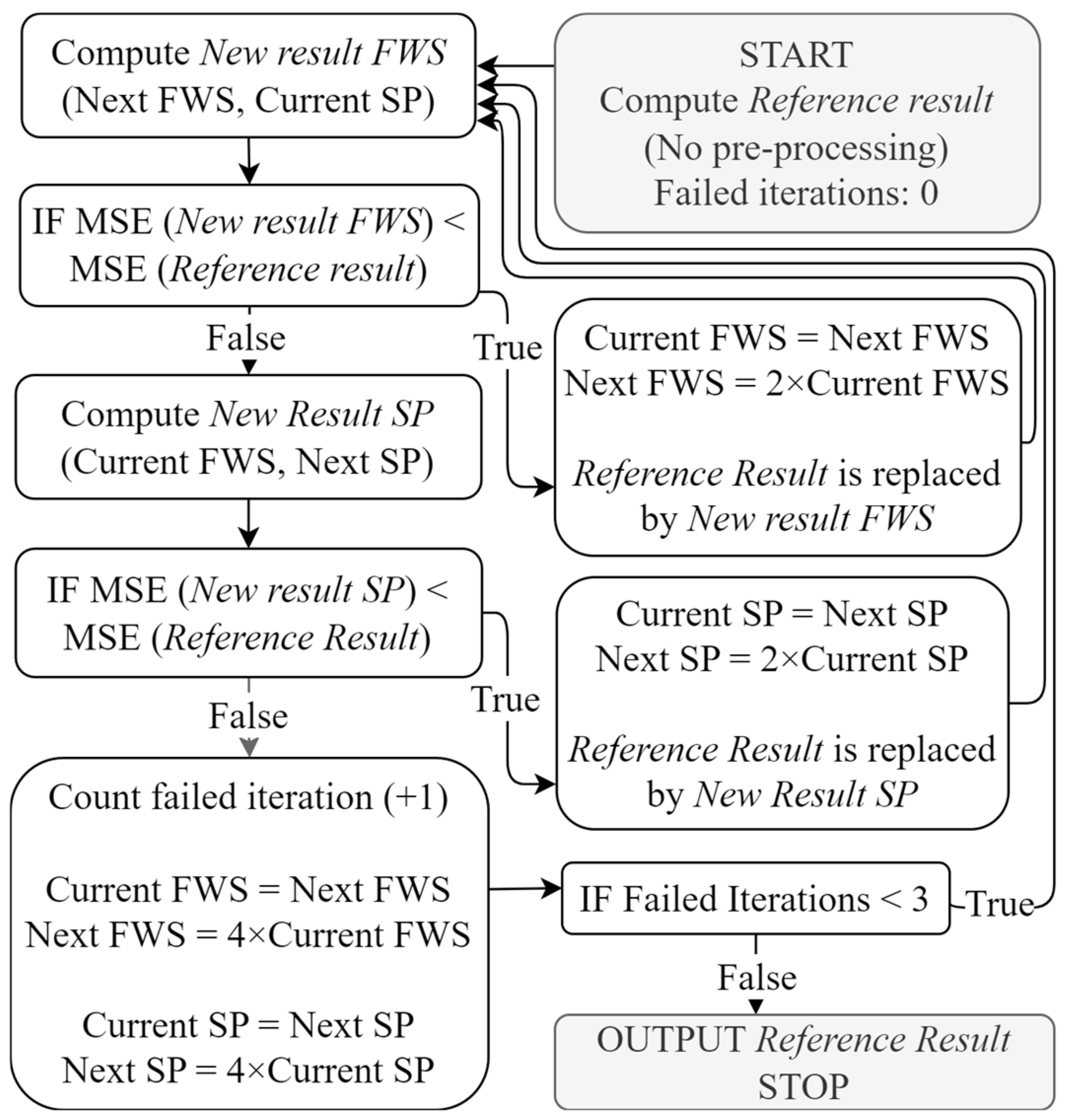
2.2.3. Extraction Based on Differential Evolution (DE-ECM)

For comparison purposes, a third process was set based on global optimization, without any alterations. The selection followed the popularity of this type of process in recent research and its potential to avoid a local minimum result in the absence of additional knowledge regarding the objective function shape. Additional motivation for the selection follows the global optimization-based procedures being considered a good standard for reliability and accuracy. All the parameters proposed for identification are set as variables for optimization and boundary values were required instead of initial values. These were set between 0 and a positive value, 10 for the Open Circuit Voltage, 1 for the resistance values, and 100 and 1000 for the time constants. By contrast with the proposed two methods, which present as deterministic, this process presents stochastic behavior. Consequently, for each sample, 10 separate runs were computed, with their average presented in the results section. The objective function used to drive the process is the same used for the LS-ARX and LS-ECM methods, while the readily available global optimizer was selected from the SciPy 1.5.4 library, namely the differential evolution (DE) algorithm [29]. The main role of this third method is to provide a representative benchmark for global optimization and a reliability standard, while also highlighting the efficiency of the method for applications where the model equations are ignored and not used to inform the parametrization method.

2.3. Experimental

The methods proposed for comparison were subject to assessment using experimental data. While the dataset obtained captures step discharges at SOC from 100% to 5% for 9 different temperatures, the dataset was not designed specifically for this activity, but also for more comprehensive modeling tasks. Also, despite the step response not being representative of any in-vehicle operation conditions, this format represents a very common type of data used for parameter extraction and implicit model parametrization following well-established system identification procedures. For the results presented in this work, a list of 3 short step responses (10 s) and 3 long constant current discharge steps (approximately 334 s) were selected. The resulting set was considered sufficient to demonstrate the working principle as well as compare the accuracy and efficiency of the processes.

The data were obtained from a pristine 3000 mAh NCA Sony VTC6 cell placed in an 18650 cell holder, as illustrated in Figure 4. The complete experimental setup displaying all the connections to the cell is also captured in Figure 5. To avoid imperfect contact between the plates of the holder and the cell, silver conductive was coated on contact surfaces before assembly. The cell was connected to equipment by having one set of wires (green and yellow) soldered to the plates of the holder on the opposite face to the contact surface with the cell to draw current, while wires intended to measure voltage (red/black) were soldered to the plates next to the point of contact with the cell, in an attempt to minimize overlap of the two circuits.

The cell was connected to a programmable electronic load manufactured by EA Elektro-Automatik GmbH & Co. KG, Viersen, Germany, model EA-EL 3080-60 B, to accurately control the discharge current. The second set of wires was connected to two multimeters set in parallel, manufactured by Tektronix, Inc., Beaveron, OR, USA, model Keithley 2110 5 ½; this double voltage measurement setup was selected to avoid data loss in the case of a malfunction. The electronic load was controlled using the manual built-in interface, while the multimeters could feed the measured data directly to a computer. The computer interface for the multimeters was built as a Python 3.9.13 script based on Py-VISA 1.13.0 [30] and developed specifically for this activity. Lastly, a third multimeter was connected to a K-type thermocouple attached to the surface of the cell using thermally conductive adhesive and electrical tape, with the purpose of monitoring and controlling the temperature of the cell as well as recording it. Highly precise control of the sampling rate was not possible with the equipment available, either with the Python script developed or by using the proprietary software available for the multimeters. By considering the penalty in accuracy, the sample rate of the data was at approximately 20 Hz for the voltage measurements, while it was set to approximately 1.6 Hz for temperature. Further details about thermal control and monitoring are not considered relevant in this study as the data used were obtained in ambient conditions considered to be 20 °C.

The structure of one test at one specific temperature point is summarized in Figure 6 and follows charging the cell to 100%, defined as a 20 mA cut-off current at a constant voltage of 4.2 V, defined by the manufacturer in ambient conditions (20 °C). The charging is followed by a relaxation period of 30 min and another constant voltage charging to the same cut-off current value, which is added to avoid false SOC points due to hysteresis. This is followed by another relaxation period of a minimum of 30 min while the cell was conditioned to the correct temperature.

The test is commenced by a 10 s pulse discharge at 1C (−3A) associated with 100% SOC, which is then followed by 15 min of relaxation. The SOC points are then changed by 5% and 10% increments to the following values: 95, 85, 75, 65, 55, 45, 35, 25, 15, 10, and 5, once again using constant current at the same value of 1C. After discharging to the SOC point, a minimum period of 30 min of relaxation is allowed, after which the 10 s pulse is applied again, followed by 15 min of relaxation. After the last SOC point is observed under the pulse, the cell is completely discharged to 0%, defined as a −35 mA cut-off current at a constant voltage of 2.5 V. Through coulomb counting, this complete discharge is used to confirm the SOC breakpoints in the time series. Exemplification of the data employed is presented by the time seriesdisplayed in Figure 7. Segments numbered 1 to 3 (S1 to S3) capture individual segments associated with 10 s pulses, while segments 4 to 6 (S4 to S6) capture 10% SOC discharge steps.

3. Results

The accuracy and efficiency of each method represent the first main observations.

Table 2. Mean squared error (MSE) results.

Sample No.	SOC Range	Discharge Time (s)	LS-ARX	LS-ECM	DE-ECM (Average)
Sample 1	24.6–24.3%	10 s	5.349 × 10−7	5.900 × 10−8	5.890 × 10−8
Sample 2	64.8–64.5%	10 s	4.164 × 10−7	4.661 × 10−8	4.660 × 10−8
Sample 3	95.0–94.7%	10 s	5.971 × 10−7	3.798 × 10−7	3.794 × 10−7
Sample 4	24.3–14.6%	~334 s	1.082 × 10−4	4.825 × 10−6	4.826 × 10−6
Sample 5	64.5–54.8%	~334 s	2.120 × 10−5	8.061 × 10−7	8.058 × 10−7
Sample 6	94.7–84.9%	~334 s	2.391 × 10−5	7.069 × 10−6	7.073 × 10−6

summarizes the mean squared error (MSE) achieved by each of the methods proposed. A comparison of the measured data against the simulated response as well as the profile of the mean absolute error (MAE) have been presented for samples 1 and 4 in Figure 8 and Figure 9 to further illustrate the results of the process, with highlights over regions of interest. The inclusion of only one result for each type of sample followed the similarity of the results across the same type of sample, leading to a lack of additional insight following plots using the same template. The results illustrated confirm a very close match between the results of the LS-ECM and DE-ECM method, which is also further supported by the convergence to highly similar parameter values between the two procedures summarized for sample 6 in

Table 3. Parameter values obtained for sample 6.

Parameter	LS-ARX	LS-ECM	DE-ECM (Average)
$V_{OC,max}$ (V)	4.103	4.108	4.108
$V_{OC,min}$ (V)	4.075	4.076	4.076
$R_0$ (Ω)	2.513 × 10−2	2.666 × 10−2	2.670 × 10−2
$R_1$(Ω)	1.011 × 10−2	1.434 × 10−2	1.437 × 10−2
${\tau }_1$ (s)	3.850	13.788	13.938
$R_2$ (Ω)	2.240 × 10−2	1.668 × 10−2	1.664 × 10−2
${\tau }_2$ (s)	95.961	183.044	184.345

. The same comparisons in Table 2 and Table 3 as well as Figure 8 and Figure 9 also indicate the LS-ARX procedure is substantially less accurate.

Targeting an efficiency perspective, the evolution of all three algorithms is also presented in Figure 10 for sample 1, while

Table 4. Number of objective function evaluations.

Sample No.	LS-ARX (% of DE-ECM)	LS-ECM (% of DE-ECM)	DE-ECM (Average)
Sample 1	19 (0.15%)	311 (2.42%)	12,836 (100%)
Sample 2	25 (0.17%)	161 (1.12%)	14,398 (100%)
Sample 3	20 (0.13%)	223 (1.48%)	15,107 (100%)
Sample 4	9 (0.08%)	121 (1.10%)	10,983 (100%)
Sample 5	7 (0.05%)	163 (1.15%)	14,129 (100%)
Sample 6	18 (0.16%)	77 (0.67%)	11,367 (100%)

summarizes the number of objective function evaluations for all samples. In addition to the absolute value, the number of evaluations was also expressed in percentages relative to the values indicated for the DE-ECM process. The results highlight the LS-ARX as the most effective from the perspective of computational expense due to its lowest MSE during the initial iterations. Nevertheless, the process also presents the lowest amount of improvement, leading to results with the highest final MSE. These attributes recommend the procedure to be more suited for value estimation tasks than highly accurate parameter extraction. This statement is also supported by the fact that the procedure requires no starting values while being able to compute all parameter values with one single computation.

The DE-ECM method can be observed as having the highest computational effort to converge to a satisfactory result. By considering the comparison study presented by Hou et al. [21], the evolution of the DE algorithm is representative of a global solver. Nevertheless, it should also be noted that substantial variations can be caused by the starting values and boundaries as well as the stochastic components in the optimization. The LS-ECM procedure presents the best compromise, with results directly comparable with global optimization, but with only a fraction of the computational cost, endorsing the procedure as highly effective in obtaining accurate results.

The results presented for the DE-ECM process in this section represent the average values obtained across the 10 runs computed for each sample. While the process has consistently converged to the same minimum point for all samples, the number of iterations required varied. Across all runs, the average percentage deviation was 7.942%, while the largest difference was found to be 25.678%, observed for one of the runs computed for sample 6. By contrast, the average percentage deviation for MSE, at 0.044%, was considered almost insignificant. For parameters, using sample 6 for exemplification, the values followed the sensitivity of the voltage response with respect to the type of parameter. As a result, the average for Open Circuit Voltage was found to be 8.173 × 10⁻⁴%, for resistance values the average was 0.532%, while the highest average, at a value of 2.533%, was presented for time constants.

4. Discussion

4.1. Analysis of LS-ARX Procedure

Without any preprocessing in the cases presented, the initial LS-ARX results will be likely biased towards the high-frequency behavior found in the data. Applying a moving average filter has the benefit of not only removing noise from the data but also dampening the high-frequency dynamics captured, consequently making the slow dynamics increasingly more observable. In return, the slow time constants influence a higher percentage of the data and are more effective in reducing the MSE values driving the process. The downsampling process creates a similar transition, however, by adding simplification of the response signal. Accidental aliasing can also potentially benefit the same transition as the selection of the filter window size and the downsampling process is performed iteratively and not analytically. Despite improvement, the LS-ARX method still presents the least accurate results, as the issues identified in Section 2.2.1 are reduced by the optimization-type process, but not completely removed.

The results in

Table 5. Global optimum preprocessing settings.

Sample No.	Default MSE	Best Result MSE	Filter Window Size	DS Factor	Global Minimum MSE
Sample 1	1.611 × 10−6	5.349 × 10−7	2048	2	5.316 × 10−7
Sample 2	2.334 × 10−6	4.164 × 10−7	2048	16	4.043 × 10−7
Sample 3	2.994 × 10−6	5.971 × 10−7	1024	4	5.971 × 10−7
Sample 4	1.085 × 10−4	1.082 × 10−4	1	2	1.082 × 10−4
Sample 5	2.120 × 10−5	2.120 × 10−5	1	1	1.705 × 10−5
Sample 6	3.150 × 10−5	2.391 × 10−5	64	8	2.226 × 10−5

summarizing the values for filter window size and the magnitude of the downsampling (DS) process associated with the lowest error highlight that data segments containing short discharge steps (samples 1 to 3) benefit more from the optimization approach and reach the upper limit for the filter window size. By contrast, the long discharge pulses (samples 4 to 6) gain significantly less from the optimization approach, as only results from sample 6 present a significant improvement. One potential cause for this difference can be traced back to a reduced capability of the model to replicate the data caused by the long data segments containing more complex nonlinear behavior. In the case of LS applied to the ARX format, the margin between the model and data can also be considered to have a similar effect on error propagation. Nevertheless, as the preprocessing is intended to mostly attenuate high-frequency parts of the voltage signal, it will be ineffective in bringing an improvement for this separate cause. Attempting to find parameter values for two RC elements, which may present a significant gap in time scales using the same preprocessing setting, may also have a negative effect set to be reduced by a model decoupling-type approach.

To further investigate the limitations of the process, the results in Table 5 have also been enhanced with the global minimum achievable using the LS-ARX method. The complete mapping of the MSE error for sample 6 is presented in Figure 11. These bring to attention an additional limitation of the search algorithm employed, namely the very rudimentary optimization procedure of the preprocessing settings, which will likely converge to the local minima. Nevertheless, with the exemption of sample 5, the results are still comparable to the global MSE and require substantially fewer evaluations than evaluating all possible combinations.

The variation in MSE relative to the preprocessing settings illustrated in Figure 11 also suggests the procedures employed as potential limiting factors. The selection of moving average filtering and downsampling directly influence the shape of the MSE and may result in a shape with multiple local minima requiring to be found and evaluated. As a result, preprocessing methodologies such as frequency domain filters and decimation should also be considered as alternatives. Their efficiency should be evaluated in relation to LS-ARX using the achievable MSE as well as its shape relative to the parameters controlling them.

4.2. Analysis of LS-ECM Procedure

The second procedure introduced in this study endorses the application of the same LS process directly to the default state-space format of the model. The results present this approach as marginally less accurate in comparison to the one achieved by the DE-ECM procedure considered as a benchmark. The similarity of the results can be attributed to the shared elements between the two methodologies, such as the objective function and the iterative structure cascading information from one cycle to the next. The substantial gap in computation performance summarized by Table 4 also presents the main differentiator that caused the ability of the LS-ECM to include gradient information.

Nevertheless, the integration of a gradient-based approach for the second step of the LS-ECM means the capability of converging correctly is present only in the case of local optimization. The similarity between the results presented by the LS-ECM and DE-ECM for all six samples presents the first suggestion of correct convergence towards the global minima, and implicitly for the optimization problem to only present one local minima. For confirmation, additional examination of the procedure brought further evidence to support this hypothesis and prove the correct application of the process.

Figure 12 illustrates the shape of the objective function in the case of sample 6 during the last iteration, relative to the nonlinear parameters optimized in step 2 of the procedure. Step 1 parameters were not included as they are linear parameters, which will not reveal any risk of local minimum values being present. The shape of the objective function, despite presenting variability caused by the data segment, will consistently feature a main global minimum and a number of additional local minima dependent on the order of the RC model. In the case of the 2RC, only one additional local minima is present. For each set of linear parameters, a global minimum will be present, while a second will result from a potential inversion of the time constant values between them. As a result, the shape will present a degree of symmetry directly linked with the relation between the resistance values associated with the RC element (perfect symmetry will be caused by two equal values). It should be noted also that converging to the local minima instead of the global is not possible since each iteration of the first step in the process will set the resistance values to the global minimum for the current values of the time constants. This will lead to a global minimum occurring in the MSE surface created for step 2 in the proximity of their current values, rather than the mirrored part, supporting the optimization problem being correctly classified as local. It should be noted that an additional requirement for the process to function in the described manner is for the data points to be equidistant in the time axis, as the presence of data spaced unequally will introduce additional local minima points. Such unequal spacing can result from data compression algorithms and should be corrected as a preprocessing step.

The surface illustrated in Figure 12 also highlights a separate limitation, namely the convergence, which is naturally dependent on the gradient of the objective function. This will affect convergence speed and overall robustness since small gradients will reduce significantly the efficiency of the process. In the extreme, gradients that approach zero present the risk of instability caused by insufficient precision in the computation. The potential issue created by gradient should also be accounted for during initialization; in the current study, the lower bound of 0 for the time constant values encouraged initial values relatively close to this value. This increased the likelihood of undervalued time constant parameters effective in lowering MSE quickly as they increase, meaning a sufficiently observable gradient for the computations to be stable.

5. Conclusions

Two new methodologies for the identification of ECM parameters from battery systems data based on least squares linear regression (LS) have been proposed, analyzed and compared against a third indicated by prior research as a benchmark and represented by global optimization, namely differential evolution. Both methods presented satisfactory results as well as a trade-off between the effort and knowledge required to set up, computational effort, and accuracy of results. The best compromise is represented by the LS-ECM process employing the application of the linear solver directly to the state-space discrete equations of the model. The process is enabled by effective linearization for the nonlinear parameters through recursive computation of the total derivative. This procedure presented limited computational effort and knowledge to set up while producing nearly identical results with respect to the global optimization in terms of accuracy. The highest MSE of 3.798 × 10⁻⁷ V² and 7.069 × 10⁻⁶ V² was obtained over short and long pulses of the current part of cell-level data obtained from a Sony VTC6 cell. The match between the results of the process and the results of the global optimization also suggests that the error is caused by the capability of the model to replicate the system (linear response assumption) rather than the parameter identification method employed.

By comparison, the LS-ARX process presented as the fastest, while also extracting parameter values directly from data, without any assumption over the starting values. Nevertheless, the limitations presented by the recursive equations of the model result in penalties in accuracy, making this method recommendable for fast extraction of parameter estimates to be further refined. The DE-ECM process is the most robust and accurate solution, as well as the easiest to set up, but also very computationally expensive, potentially prohibiting the use of the procedure in the case of large datasets.

Future work will target the implementation of the extraction methods to build a complete battery system model, and is set to include the nonlinear behavior associated with temperature, SOC, and current amplitude. Moreover, a more efficient extraction procedure can balance the benefits of the proposed methods by setting the starting point for the LS-ECM by using the LS-ARX. A more comprehensive understanding of the reduction in computational effort may be provided by adding to the comparison a state-of-the-art local optimization, while each procedure also represents the base for further enhancements. In the case of the LS-ARX process, alternative optimization and preprocessing procedures may present interest. For LS-ECM, hybridization with a different optimization structure may focus on accelerated convergence, reducing the gradient-induced issues in relation to starting points and convergence speed. Lastly, the LS-ECM procedure may also present interest as the fundamental element supporting an alternative RLS-type procedure.

References

1. Kalogiannis, T.; Hosen, M.S.; Sokkeh, M.A.; Goutam, S.; Jaguemont, J.; Jin, L.; Qiao, G.; Berecibar, M.; Van Mierlo, J. Comparative Study on Parameter Identification Methods for Dual-Polarization Lithium-Ion Equivalent Circuit Model. Energies 2019, 12, 4031. [Google Scholar] [CrossRef]
2. Li, J.; Peng, Y.; Wang, Q.; Liu, H. Status and Prospects of Research on Lithium-Ion Battery Parameter Identification. Batteries 2024, 10, 194. [Google Scholar] [CrossRef]
3. Ljung, L. System Identification; Webster, J.G., Ed.; Wiley Encyclopedia of Electrical and Electronics Engineering: Hoboken, NJ, USA, 1999. [Google Scholar] [CrossRef]
4. Zhang, T.; Guo, N.; Sun, X.; Fan, J.; Yang, N.; Song, J.; Zou, Y. A Systematic Framework for State of Charge, State of Health and State of Power Co-Estimation of Lithium-Ion Battery in Electric Vehicles. Sustainability 2021, 13, 5166. [Google Scholar] [CrossRef]
5. Huang, C.-S. Online Parameter Identification for Lithium-Ion Batteries: An Adaptive Moving Window Size Design Methodology for Least Square Fitting. IEEE Trans. Veh. Technol. 2023, 72, 5824. [Google Scholar] [CrossRef]
6. Raihan, S.A.; Balasingam, B. Recursive Least Square Estimation Approach to Real-Time Parameter Identification in Li-ion Batteries. In Proceedings of the 2019 IEEE Electrical Power and Energy Conference (EPEC), Montreal, QC, Canada, 16–18 October 2019. [Google Scholar] [CrossRef]
7. Kim, M.; Kim, K.; Han, S. Reliable Online Parameter Identification of Li-Ion Batteries in Battery Management Systems Using the Condition Number of the Error Covariance Matrix. IEEE Access 2020, 8, 189106. [Google Scholar] [CrossRef]
8. Fan, Y.; Shi, H.; Wang, S.; Fernandez, C.; Cao, W.; Huang, J. A Novel Adaptive Function—Dual Kalman Filtering Strategy for Online Battery Model Parameters and State of Charge Co-Estimation. Energies 2021, 14, 2268. [Google Scholar] [CrossRef]
9. Xia, B.; Huang, R.; Lao, Z.; Zhang, R.; Lai, Y.; Zheng, W.; Wang, H.; Wang, W.; Wang, M. Online Parameter Identification of Lithium-Ion Batteries Using a Novel Multiple Forgetting Factor Recursive Least Square Algorithm. Energies 2018, 11, 3180. [Google Scholar] [CrossRef]
10. Sun, X.; Ji, J.; Ren, B.; Xie, C.; Yan, D. Adaptive Forgetting Factor Recursive Least Square Algorithm for Online Identification of Equivalent Circuit Model Parameters of a Lithium-Ion Battery. Energies 2019, 12, 2242. [Google Scholar] [CrossRef]
11. Sun, C.; Lin, H.; Cai, H.; Gao, M.; Zhu, C.; He, Z. Improved parameter identification and state-of-charge estimation for lithium-ion battery with fixed memory recursive least squares and sigma-point Kalman filter. Electrochim. Acta 2021, 387, 138501. [Google Scholar] [CrossRef]
12. Li, C.; Kim, G.-W. Improved State-of-Charge Estimation of Lithium-Ion Battery for Electric Vehicles Using Parameter Estimation and Multi-Innovation Adaptive Robust Unscented Kalman Filter. Energies 2024, 17, 272. [Google Scholar] [CrossRef]
13. Xu, Y.; Chen, X.; Zhang, H.; Yang, F.; Tong, L.; Yang, Y.; Yan, D.; Yang, A.; Yu, M.; Liu, Z.; et al. Online identification of battery model parameters and joint state of charge and state of health estimation using dual particle filter algorithms. Int. J. Energy Res. 2022, 46, 19615–19652. [Google Scholar] [CrossRef]
14. Tian, N.; Wang, Y.; Chen, J.; Fang, H. On parameter identification of an equivalent circuit model for lithium-ion batteries. In Proceedings of the IEEE Conference on Control Technology and Applications (CCTA), Maui, HI, USA, 27–30 August 2017. [Google Scholar] [CrossRef]
15. Tran, M.-K.; DaCosta, A.; Mevawalla, A.; Panchal, S.; Fowler, M. Comparative Study of Equivalent Circuit Models Performance in Four Common Lithium-Ion Batteries: LFP, NMC, LMO, NCA. Batteries 2021, 7, 51. [Google Scholar] [CrossRef]
16. Chen, C. Parameter Determination for the Battery Equivalent Circuit Model Using a Numerical Integro-Differential Method; SAE Technical Paper 2020-01-1179; SAE International: Warrendale, PA, USA, 2020. [Google Scholar] [CrossRef]
17. Al Rafei, T.; Yousfi Steiner, N.; Chrenko, D. Genetic Algorithm and Taguchi Method: An Approach for Better Li-Ion Cell Model Parameter Identification. Batteries 2023, 9, 72. [Google Scholar] [CrossRef]
18. Zhou, S.; Liu, X.; Hua, Y.; Zhou, X.; Yang, S. Adaptive model parameter identification for lithium-ion batteries based on improved coupling hybrid adaptive particle swarm optimization- simulated annealing method. J. Power Sources 2021, 482, 228951. [Google Scholar] [CrossRef]
19. Ghoulam, Y.; Mesbahi, T.; Wilson, P.; Durand, S.; Lewis, A.; Lallement, C.; Vagg, C. Lithium-Ion Battery Parameter Identification for Hybrid and Electric Vehicles Using Drive Cycle Data. Energies 2022, 15, 4005. [Google Scholar] [CrossRef]
20. Cheng, Y.S. Identification of Parameters for Equivalent Circuit Model of Li-Ion Battery Cell with Population Based Optimization Algorithms. Available online: https://ssrn.com/abstract=4229575 (accessed on 14 September 2024).
21. Hou, J.; Wang, X.; Su, Y.; Yang, Y.; Gao, T. Parameter Identification of Lithium Battery Model Based on Chaotic Quantum Sparrow Search Algorithm. Appl. Sci. 2022, 12, 7332. [Google Scholar] [CrossRef]
22. Lee, S.; Lee, D. A Novel Battery State of Charge Estimation Based on Voltage Relaxation Curve. Batteries 2023, 9, 517. [Google Scholar] [CrossRef]
23. Lee, J.; Sun, H.; Liu, Y.; Li, X. A machine learning framework for remaining useful lifetime prediction of li-ion batteries using diverse neural networks. Energy AI 2024, 15, 100319. [Google Scholar] [CrossRef]
24. Cleary, T.; Nozarijouybari, Z.; Wang, D.; Wang, D.; Rahn, C.; Fathy, H.K. An Experimentally Parameterized Equivalent Circuit Model of a Solid-State Lithium-Sulfur Battery. Batteries 2022, 8, 269. [Google Scholar] [CrossRef]
25. Zeigler, B.; Muzy, A.; Kofman, E. Chapter 3—Modeling Formalisms and Their Simulators. In Theory of Modeling and Simulation, 3rd ed.; Zeigler, B., Muzy, A., Kofman, E., Eds.; Academic Press: Cambridge, MA, USA, 2019; pp. 43–91. [Google Scholar]
26. Cheever, E. The Z Transform. 2022. Available online: https://lpsa.swarthmore.edu/ZXform/FwdZXform/FwdZXform.html (accessed on 14 September 2024).
27. Cheever, E. Transformation: Transfer Function ↔ State Space. 2022. Available online: https://lpsa.swarthmore.edu/Representations/SysRepTransformations/TF2SS.html (accessed on 14 September 2024).
28. SciPy. Scipy.optimize.lsq_linear—SciPy v1.10.1 Manual. 2023. Available online: https://docs.scipy.org/doc/scipy/reference/generated/scipy.optimize.lsq_linear.html (accessed on 14 September 2024).
29. SciPy. Scipy.optimize.differential_evolution—SciPy v1.10.1 Manual. 2023. Available online: https://docs.scipy.org/doc/scipy/reference/generated/scipy.optimize.differential_evolution.html (accessed on 14 September 2024).
30. PyVisa Authors. PyVISA—Control Your Instruments with Python, PyVISA. 2023. Available online: https://pyvisa.readthedocs.io/en/latest/index.html (accessed on 14 September 2024).
Figure 1. Double polarization ECM diagram.
Batteries 10 00343 g001
Figure 2. LS-ARX process flow diagram (FWS—filter window size; SP—sampling period).
Batteries 10 00343 g002
Figure 3. LS-ECM process flow diagram.
Batteries 10 00343 g003
Figure 4. Sony VTC6 cell setup.
Batteries 10 00343 g004
Figure 5. Experimental setup diagram.
Batteries 10 00343 g005
Figure 6. Battery cell data acquisition procedure flow diagram.
Batteries 10 00343 g006
Figure 7. Sony VTC6 voltage response data (20 °C).
Batteries 10 00343 g007
Figure 8. Sample 1 results. (a) Measured vs. simulated voltage; (b) voltage absolute error profile.
Batteries 10 00343 g008
Figure 9. Sample 4 results. (a) Measured vs. simulated voltage; (b) voltage absolute error profile.
Batteries 10 00343 g009
Figure 10. MSE evolution results (minimum MSE after each evaluation for sample 1).
Batteries 10 00343 g010
Figure 11. MSE function shape for sample 6—LS-ARX process (MSE limited at 10−5).
Batteries 10 00343 g011
Figure 12. MSE function shape for sample 6—LS-ECM process (step 2; cycle 38).
Batteries 10 00343 g012