A Novel Quick Temperature Prediction Algorithm for Battery Thermal Management Systems Based on a Flat Heat Pipe

Abstract

Predicting the core temperature of a Li-ion battery is crucial for precise state estimation, but it is difficult to directly measure. Existing quick temperature-predicting approaches can hardly consider the thermal mass of complex structure that may cause time delays, particularly under high C-rate dynamic conditions. In this paper, we developed a quick temperature prediction algorithm based on a thermal convolution method (TCM) to calculate the core temperature of a flat heat pipe-based battery thermal management system (FHP-BTMS) under dynamic conditions. The model could predict the core temperature rapidly through convolution of the thermal response map which contains full physical information. Firstly, in order to obtain a high fidelity spatio-temporal temperature distribution, the thermal capacitance-resistance network (TCRN) of the FHP-BTMS is established and validated by constant and dynamic discharging experiments. Then, the response map of the core temperature motivated by various impulse heat sources and heat sinks is obtained. Specifically, the dynamic thermal characteristics of an FHP are discussed to correct the boundary conditions of the TCM. Afterwards, the temperature prediction performances of the TCM and a lumped model under different step operating conditions are compared. The TCM results show a 70–80% accuracy improvement and better dynamic adaptivity than the lumped model. Lastly, a vertical take-off and landing (VTOL) profile is employed. The temperature prediction accuracy results show that the TCM can maintain a relative error below 5% throughout the entire prediction period.

1. Introduction

With the growing demand for decarbonization, pure electric vehicles and electrification of transportation have developed rapidly in recent years [1]. The Lithium-ion battery, benefiting from its high power and energy density, is considered to be one of the most crucial and marketable technologies among electrochemical power sources [2]. A tremendous amount of research works have clarified that temperature critically influences the overall performance of Li-ion batteries, including cycled/calendar life, state of power (SOP), security, etc. [3]. A low temperature under 0 °C causes Lithium precipitation. An exorbitant temperature (above 50 °C) can lead to decomposition of the solid electrolyte interface (SEI). Therefore, an inappropriate operating temperature causes capacity degradation and increases the risk of thermal runaway [4]. Battery thermal management systems (BTMS) play a crucial role in regulating Li-ion battery temperatures within the optimal region.

The structural configurations and control strategies are two main research aspects of BTMSs. There are various types of BTMS. As the primary kinds, air cooling and liquid cooling are widely applied in electric vehicles [5,6]. In order to achieve favorable thermal management performance, the layouts between the coolant flow channel and batteries have been taken into consideration and extensively studied, as well as the optimal BTMS design methods [7,8]. As the safety requirements for battery systems and the demands of high charge/discharge rates both increase, BTMSs based on heat pipes were proposed. Profiting from the principle of latent heat during the phase change process, heat pipes can reach a high equivalent thermal conductivity and low temperature gradient on the evaporation side. Heat pipe-based BTMSs are generally combined with air or liquid cooling on the condensation side as a heat sink [9,10]. For the purpose of maintaining temperature consistency among batteries, phase change materials (PCM) are also applied together with heat pipes [11]. Researchers focused on the thermal performance of such BTMSs through sample experiments and three-dimensional Computational Fluid Dynamics (CFD) simulation. Zhang et al. [12] placed an FHP between battery cells, the temperature of which can be regulated below 32 °C under 4 C condition with an ambient temperature of 25 °C, and the temperature difference is below 5 °C. Jouhara et al. [13] placed the FHP below the battery pack. Liquid cooling was utilized in the condensation part of the FHP. The maximum temperature and temperature difference are regulated to 35 °C and 3 °C, respectively. Liu et al. [14] also applied a fin structure on a cylindrical battery pack, and their experimental results provided a quantitative relationship between cooling flow rate and temperature distribution. Although heat pipe-based BTMSs demonstrated excellent temperature regulation effectiveness, the temperature prediction methods have not developed practically yet. The CFD work costs time, and usually assumes the FHP to be a thermal conductor with constant thermal conductivity [15,16,17], without considering the dynamic thermal effects, which is essential to the accuracy of battery temperature prediction and control under dynamic operating current and variable boundary conditions.

As for control strategies, the existing research works mainly focus on systematic air-cooled and liquid-cooled BTMSs. The control targets would generally take temperature, temperature difference, calendar/cycled life-span and the energy consumption of the BTMS into consideration. Cen et al. [18] studied the influence of proportional, integral and differential (PID) parameters on control precision by combining automotive air-conditioning and battery systems. When the expected control target temperature is set to 25 °C, the temperature differences of batteries are within 2 °C at 0.5 C and 2.5 °C at 1.5 C. Min et al. [19] proposed a fuzzy control strategy based on a battery-lifetime extension method which reduces battery-lifetime loss by the peak shifting and valley filling effect. It can reduce the loss of battery life during the heating-up process under low-temperature conditions without affecting the state of temperature (SOT). Gao et al. [20] compared the dynamic performance and precision of temperature control between the fuzzy logic method and PID for an air-cooled array battery system. In the above research, temperature is the most crucial index and target for controller and strategy design. The adaptable temperature model is mostly a lumped model, which expresses battery temperature as the volume-average one. Moreover, the operating charge/discharge rate of the working condition is low as a conventional system. Due to the rolling and multi-layer structure of anode/cathode pole pieces and separators inside the battery, the normal thermal conductivity of the diaphragm is much smaller than in the other direction. Thermal inertia will lead to delays between the internal and surface temperatures. With the gradual enlargement of battery volumes and high C-rate operating conditions, this effect will be highlighted. Lee et al. [21] found that the temperature difference between inside and outside under 3 C working conditions can reach 8 °C through home-made thermocouples inserted into a pouch battery. The response delay turns out to be around 45–90 s. Hence, merely detecting the surface temperature and considering the average temperature of the battery are not enough to predict SOT precisely.

Considerable number of researches have already noticed the defects of the lumped thermal model and the inadequacy of measuring surface temperature only. Kalman filters (KF), finite element methods (FEM) and data-driven methods are the usual approaches to estimate and predict the SOT of the battery. In terms of KF methods, the internal temperature can be estimated and corrected in real time based on sensor data and a thermo-electrical model [22]. Then, extended Kalman filter (EKF), dual-KF and joint estimation were widely used to achieve higher precision [23,24,25]. However, KF-based methods essentially involve online solving and correction of thermal models. The lack of feedback will lead to inadequate accuracy during temperature prediction. As for FEM, they can accurately reconstruct the temperature field but suffer from long computation times while solving the implicit equations. Some studies have explored dimensionality reduction methods that include high-dimensional temperature information. Hu [26,27] generated a temperature–time matrix based on CFD simulation results and performed singular value decomposition to obtain temperature field snapshots. This reduced-order method significantly improves the calculation speed of obtaining a 3D temperature field, yet it essentially represents a repetitive process under the same conditions and struggles to adapt to dynamically variable boundary conditions and different initial conditions. Data-driven methods have also received attention to predict SOT in recent years. Kleiner developed a recurrent neural network, which makes the results of the previous time step temperature prediction memorable and performs with higher precision and robustness dynamically than traditional feedforward artificial neural networks [28]. Wang proposed a physical informed neural network (PINN) to achieve self-learning of the battery electoral-thermal model during aging [29]. However, such machine learning models are black-box and rely on a high-fidelity training dataset which is difficult and time-consuming to obtain [30]. Additionally, thermal network methods were widely applied for their reasonable simplification of FEM and interpretability [31], but the calculation speed cannot meet the real-time requirements when the structure of the BTMS becomes more complex. Therefore, a temperature-prediction algorithm that can reflect physical mechanisms and enable fast computation at the same time is still lacking.

In order to fill the aforementioned research gaps, this paper developed a quick temperature-prediction algorithm based on the thermal convolution method (TCM) for an FHP-based BTMS. Compared to the existing studies, three contributions are achieved. The first contribution is the theoretical modeling of dynamic heat transfer effects between the FHP and prismatic batteries, with the consideration of the phase change heat transfer mechanism. We integrate it into a thermal capacitance-resistance network (TCRN) to simulate temperature distribution. Experiments under constant and dynamic current profiles were carried out and the accuracy of the TCRN was verified. The second contribution is to propose a paradigm for temperature prediction based on the thermal convolution method. The temperature responses of the inner node of the battery to multiple heat sources are collected, and hence the inner temperature of the battery can be predicted precisely through a temporal convolutional integral so long as the boundary conditions are provided. The third contribution is the research on the influences of cooling and heating condition variation on the characteristic time of the FHP, which confirms the quick temperature prediction algorithm as a correction of the heat sink source term in the thermal convolution method. The algorithm performs on a similar time scale of calculation as the lumped model, but with much more accuracy. Afterwards, the temperature prediction performances of the TCM and the lumped model under various specific dynamic operating conditions were compared and discussed. The proposed temperature prediction method in this paper can serve as a foundation for controller and strategy design, and can be further extended to other forms of BTMS to accurately estimate and predict battery temperatures.

2. FHP-Based BTMS Electro-Thermal Coupled Model

2.1. FHP-Based BTMS

A prismatic Li-ion battery module combined with FHP-based thermal management system is presented in Figure 1. Twelve battery cells are closely aligned along the thickness direction, and a flexible heat-conduction pad made of silica gel is sandwiched between each two cells. The FHP is placed underneath the cells. The part of the FHP surface attached to the cells is coated with silicone grease to reduce contact thermal resistance and reinforce heat transfer. The other part of the FHP provides heat dissipation measures, and consists of a fin and an axial fan. The operating principle of the FHP-based BTMS is also shown in Figure 1. An FHP can be divided into the shell, a porous capillary wick and a vapor chamber [32].

For the above configuration of an FHP-based BTMS, the heat transfer process of the whole system includes three important aspects: (1) Operating conditions and heat generation rates of the battery module. (2) Heat transfer performance of the FHP. (3) The cooling capacity of the condensation section. According to references [33,34], the heat transfer performance of the FHP is mainly affected by heat source conditions and structural parameters. The heat transfer capacity of the FHP directly affects the temperature uniformity and cooling/heating rate of the battery module. For the fin structure and fluid channel at the condensation section of the FHP, shown in Figure 1, the cooling method can be direct air cooling or liquid cooling. In the present study, air cooling was adopted.

As indicated above, the temperature of batteries is mainly determined by both heat generation and heat dissipation. In the current section, the heat generation model of batteries and the heat transfer model of the FHP are established, respectively. Then, the coupling method of the models is introduced, and the battery parameters are calibrated by experiments.

In the current study, a module consisting of twelve prismatic battery cells is used for the analysis, and the parameters of the cells are presented in

Table 1. Technical parameters of the Prismatic Battery Cell (L148N50A).

Parameters	Value
Dimensions	148 mm × 26.7 mm × 98 mm
Nominal capacity	50 Ah
Energy	182.5 Wh
Nominal voltage	3.65 V
Anode material	NCM
Electrolyte material	LiPF6
Cathode material	Graphite
Mass	895 g

.

The FHP is produced with a shell made of aluminum, and the phase change medium is acetone, for its adaptability to the operating temperature range of the battery. The specific details of the FHP-BTMS are introduced in

Table 2. Details specification of the FHP-BTMS.

Parameters	Value
Shell Material of FHP	Aluminum
Wick Material of FHP	(Porous sintered) Aluminum particles
Working Fluid of FHP	Acetone
Evaporator length (each cell)	0.026 m
Condenser length of FHP	0.1 m
FHP width	0.148 m
FHP length	0.44 m
Total thickness of FHP	0.005 m
Thickness of shell	0.001 m
Thickness of wick	0.0015 m
Thickness of vapor channel	0.0015 m
Space of fin	0.01 m
Width of fin	0.08 m
Thickness of fin	0.0005 m
Wick porosity	0.48
Module overall size	440 mm × 150 mm × 103 mm
Cooling method	Axial fan
Fan size	120 mm × 120 mm × 50 mm
Max airflow rate	0.12 kg/m3

.

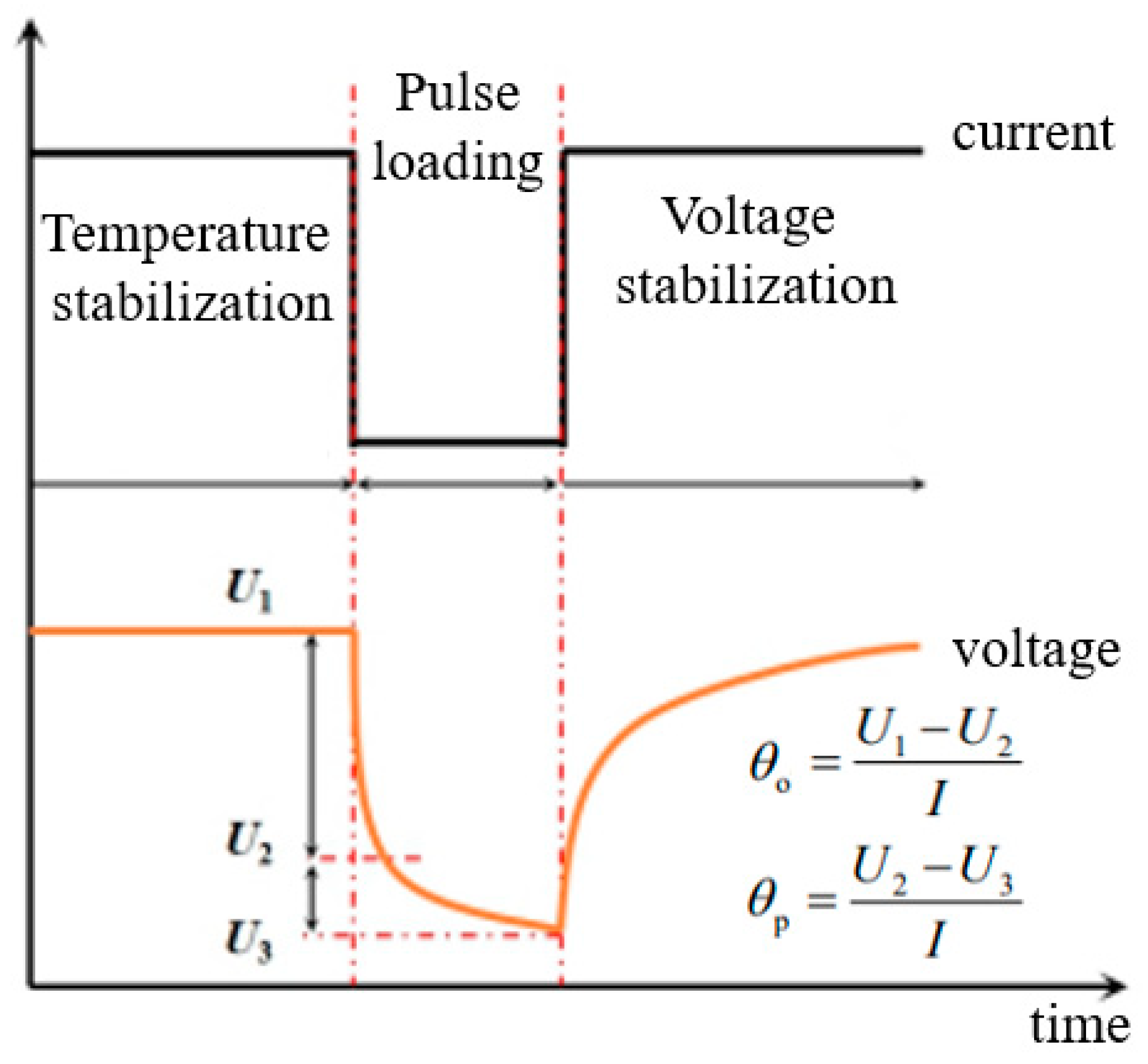
2.2. Battery Heat Generation Model

According to Newman et al. [35], the total heat generation rate inside a battery cell is composed of two parts (right side of Equation (1)): the first term refers to the irreversible heat generated during the charging-discharging process, the second term refers to the reversible heat which is produced by the electrochemical reactions.

$$Q=I(U-U_{\mathrm{ocv}})+IT\frac{\mathrm{d}{U}_{\mathrm{ocv}}}{\mathrm{d}T}$$

(1)

where I is the charging/discharging current through the battery, T is the battery temperature, U and U_ocv are the terminal voltage and open-circuit voltage of the battery, respectively. Since U_ocv is related to State of Charge (SOC), battery temperature and entropy change, a resistance-based heat generation model could be adopted to calculate the irreversible heat in order to simplify calculations. Thus, Equation (1) could be changed into:

$$Q=I^2\left({\theta }_{\mathrm{p}}\left(T,\mathrm{SOC},I\right)+{\theta }_{\mathrm{o}}\left(T,\mathrm{SOC},I\right)\right)+IT\frac{\mathrm{d}{U}_{\mathrm{ocv}}}{\mathrm{d}T}$$

(2)

where θ_p and θ_o are, respectively, the polarization resistance and ohmic resistance.

For different batteries, experiments should be carried out to obtain resistances and open circuit voltages (OCV) under different conditions, and thus the dynamic heat generation rate in a battery could be described. Hybrid pulse power characteristic (HPPC) experiments are conducted with the conditions of 10 °C, 20 °C, 30 °C and 40 °C environmental temperature, 0.5 C, 1 C, 1.5 C, 2 C charge and discharge current, respectively. As shown in Figure 2, after a certain period of pulse current (10 s in this paper), the voltage response of the battery will be excited, firstly jumping down from U₁ to U₂, and then slowly decreasing to U₃. After the end of pulse loading, the voltage starts with a jump rebound and then slowly increases. Correspondingly, the sudden change of voltage from U₁ to U₂ and the decrease from U₂ to U₃ are caused by θ_o and θ_p, respectively. According to ohmic law, the θ_o and θ_p under the tested conditions can be obtained, and the total resistance (θ_o + θ_p) of the battery can be obtained. Then, the polynomial fitting relationship of (θ_p + θ_o) and dU_ocv/dT with respect to temperature, SOC, I based on experimental results is shown in Equations (3) and (4).

$${\theta }_p+{\theta }_o=\{\begin{array}{l}{\displaystyle \sum _{i=1}^3{A}_i{\mathrm{SOC}}^i}+{\displaystyle \sum _{i=1}^3{B}_i{T}^i}++{\displaystyle \sum _{i=1}^3{C}_i{I}^i}+\\ D_1\mathrm{SOC}\cdot {T+D}_{2}T\cdot {I+D}_3\mathrm{SOC}\cdot I+E& \mathrm{SOC}>0.3\\ {\displaystyle \sum _{i=1}^2{F}_i{\mathrm{SOC}}^i}+{\displaystyle \sum _{i=1}^2{G}_i{T}^i}++{\displaystyle \sum _{i=1}^2{H}_i{I}^i}+\\ M_1\mathrm{SOC}\cdot {T+M}_{2}T\cdot {I+M}_3\mathrm{SOC}\cdot I+N& \mathrm{SOC}\le 0.3\end{array}$$

(3)

where:

$$\left[\begin{array}{lll}{A}_1& A_2& A_3\\ B_1& B_2& B_3\\ C_1& C_2& C_3\\ D_1& D_2& D_3\end{array}\right]=\left[\begin{array}{lll}-5.022& 8.767& -4.728\\ -0.085& 8.69\times {10}^{-4}& 5.51\times {10}^{-6}\\ 0.024& -4.78\times {10}^{-4}& 3.79\times {10}^{-6}\\ 7.6\times {10}^{-3}& -1.11\times {10}^{-4}& -0.00141\end{array}\right], E = 3.325$$

$$F=\left[\begin{array}{ll}{F}_1& F_2\\ G_1& G_2\\ H_1& H_2\end{array}\right]=\left[\begin{array}{ll}2.069& -16.24\\ -0.142& 1.66\times {10}^{-3}\\ 1.022\times {10}^{-2}& 8.5\times {10}^{-5}\end{array}\right]$$

$$M=\left[M_1 M_2 M_3\right]=\left[0.082 -7.33\times {10}^{-6} 0.012\right], N = 4.069$$

$$\frac{\mathrm{d}{U}_{\mathrm{ocv}}}{\mathrm{d}T}={\displaystyle \sum _{i=1}^7{A}_i{\mathrm{SOC}}^{i-1}}$$

(4)

where:

$$A=[-69.12, 214.40, -248.0, 131.55, -32.07, 3.77,-0.27]$$

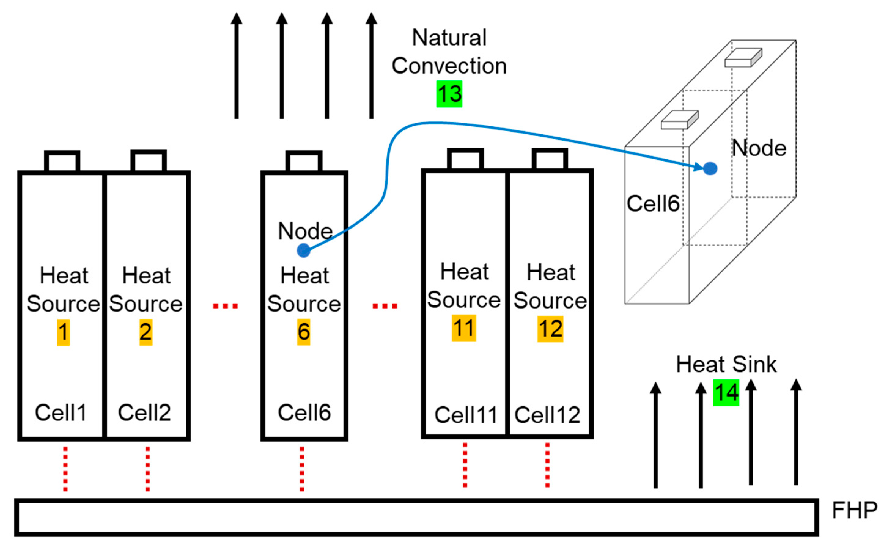
2.3. Dynamic Heat Transfer Model

The TCRN based on thermal resistance models can comparatively simplify the heat transfer analysis from complex three-dimensional CFD simulations, and is easily comprehensible; it has physical meaning and could describe the heat transfer process inside the battery module and FHP. Therefore, it is reasonable to study the regularity of battery inner temperature based on the thermal network model. In the present study, a planar multi-heat source TCRN is adopted to analyze the performance of the FHP-based BTMS. The heat transfer process along the width direction of the FHP is neglected, as it can be well considered as the thermal mass of the control volume. As shown in Figure 3, the FHP-based BTMS thermal network is subdivided into a limited number of control volumes, which refer to the nodes connected by thermal resistances. The expressions of different thermal resistance types are presented in

Table 3. Expressions of different thermal resistance types.

Type	Symbol	Expression
Conduction thermal resistance	Rc	$R_i=\frac{t_i}{{\lambda }_i{A}_i}$	(5)
	Rw
	Rs
Convection thermal resistance	Rec	$R_{eci}=\frac{1}{h_{\mathrm{si}}{A}_i}$	(6)
Phase change thermal resistance	Rpc	$R_{\mathrm{pc}i}=\frac{2-\sigma }{2\sigma }\frac{{\left(2\pi R_{\mathrm{gas}}{T}_{\mathrm{v}i}\right)}^{0.5}{R}_{\mathrm{gas}}{T}_{\mathrm{v}i}^2}{A_{\mathrm{e}i}{p}_{\mathrm{v}i}{h}_{\mathrm{fg}i}^2}$	(7)
Vapor flow thermal resistance	Rv	$R_{\mathrm{vi}}=\frac{R_{\mathrm{gas}}{T}_{\mathrm{v}i}^2}{p_{\mathrm{v}i}{h}_{\mathrm{fg}i}}\frac{12{\mu }_{\mathrm{v}i}}{t_{\mathrm{v}}^3{\rho }_{\mathrm{v}i}{w}_{\mathrm{FHP}}{h}_{\mathrm{fg}i}}{l}_{\mathrm{e}i}$	(8)

.

The thermal network structure of a single battery cell is considered firstly, and shown at the left of Figure 3, where R_cxi and R_cyi are the thermal resistance of cell structure in the x and y axis directions, respectively, and R_ei is the external thermal resistance due to natural convection or physical contact. The heat transfer process occurs in the following steps. The heat generated by two inner nodes enters the peripheral nodes through thermal conduction, then the heat is divided into four directions with three modes: (1) dissipates to the environment, (2) moves into other cells and (3) moves into the FHP. The last mode is the main basis for battery thermal management. After heat transfers through the solid shell and porous wick structure of the FHP, it enters the vapor chamber after the phase change of acetone, and finally is carried away at the condensation section.

As the state indicators of each battery cell are different, the heat generation rate must be considered mutually independent. Hence, as shown in Figure 3, there are multiple battery cells with heat sources q_c configured and the heat is transferred into the vapor chamber by the phase change process. For the proposed FHP, the corresponding thermal network model is also described in Figure 3, where R_si and R_wi, respectively, represent the thermal resistances of the shell and the wick structure, R_pci is the phase change thermal resistance and R_vi is the resistance generated due to the pressure drop along the vapor chamber.

As shown in Table 3, Equation (5) represents the thermal resistance due to solid thermal conduction. Both inter-cell and intra-cell thermal resistances in the battery module are categorized under this type. In the equation, t represents the thickness controlling the direction of heat conduction, A denotes the cross-sectional area for heat conduction and λ represents the solid thermal conductivity. Additionally, the heat transfer processes in the shell and the wick of the FHP are also considered to be based on solid thermal conduction. The thermal conductivity of the wick λ_w is obtained based on the assumption of a porous sintered material filled with liquid medium, as shown in the following equation [36]:

$${\lambda }_{\mathrm{w}}={\lambda }_{\mathrm{s}}\frac{2+{\lambda }_{\mathrm{l}}/{\lambda }_{\mathrm{s}}-2\phi \left(1-{\lambda }_{\mathrm{l}}/{\lambda }_{\mathrm{s}}\right)}{2+{\lambda }_{\mathrm{l}}/{\lambda }_{\mathrm{s}}+\phi \left(1-{\lambda }_{\mathrm{l}}/{\lambda }_{\mathrm{s}}\right)}$$

(9)

where λ_l represents the thermal conductivity of the liquid-phase working fluid, λ_s represents the thermal conductivity of the solid-phase material and φ denotes the porosity of the porous wick.

Equation (6) represents the convective thermal resistance, which includes the forced convection between the FHP fins and the cooling air, as well as the natural convection between the battery and the ambient environment. The equivalent convective heat transfer coefficient of the fins on condensing section of the FHP is calculated by following Equation (10) [37]:

$$h_{\mathrm{fin}}=0.134\frac{{\lambda }_{\mathrm{f}}}{d_{\mathrm{e}}}{\mathrm{Re}}_{\mathrm{f}}^{0.681}{\mathrm{Pr}}_{\mathrm{f}}^{1/3}{\left(\frac{s_{\mathrm{fin}}}{w_{\mathrm{fin}}}\right)}^{0.2}{\left(\frac{s_{\mathrm{fin}}}{t_{\mathrm{fin}}}\right)}^{0.1134}$$

(10)

where λ_f represents the thermal conductivity of the cooling fluid. d_e represents the hydraulic diameter of the flow channel. Re_f and Pr_f, respectively, represent the Reynolds number and Prandtl number of the cooling fluid. s_fin, w_fin and t_fin are, respectively, the space, width and thickness structure parameters of the fin, whose values have been shown in Table 2.

As the contact surface between the battery module and the FHP is only the bottom of the cells, the impact of natural convection with air on other surrounding surfaces needs to be considered. The heat transfer coefficient is calculated using the following equation [38]:

$$h_{\mathrm{air}}=\frac{\mathrm{Nu}{\lambda }_{\mathrm{air}}}{l}=0.664{\left(\frac{{\rho }_{\mathrm{air}}{v}_{\mathrm{air}}l}{{\mu }_{\mathrm{air}}}\right)}^{\frac{1}{2}}{\left(\frac{{\mu }_{\mathrm{air}}{c}_{p,\mathrm{air}}}{{\lambda }_{\mathrm{air}}}\right)}^{\frac{1}{3}}\frac{{\lambda }_{\mathrm{air}}}{l}$$

(11)

where Nu represents the Nusselt number of the cooling fluid. l represents the characteristic length of the cooling flow. The middle two terms, respectively, calculate the Reynolds number and Prandtl number based on the physical parameters of air.

Equation (7) represents the phase-change thermal resistance between the control volume of the wick and the vapor chamber. In this study, it is assumed that the heating heat flux in the evaporation section has not caused the working fluid within the wick to reach the boiling stage. Evaporation only occurs at the gas–liquid interface, and the evaporation rate is considered to be averaged within a control volume. In the equation, σ is the adjustment factor, with a value of 0.03 [39]. P_v and T_v represent the pressure and temperature at the evaporation interface, respectively. R_gas is the gas constant, and h_fgi represents the phase change latent heat of the working fluid.

Equation (8) represents the thermal resistance of steam flow between the vapor chamber control volumes. The following assumptions were made. Regarding the gas flow within the vapor chamber, assumptions of laminar and incompressible flow were made, as well as one-dimensional flow. In the equation, l_FHP represents the total length of the flat heat pipe along the heat transfer direction. Μ denotes the dynamic viscosity of the vapor, and t_v represents the thickness of the vapor chamber in the FHP.

The node temperature of the TCRN can be calculated based on the thermal balance equation:

$$c_i{\rho }_i{V}_i\frac{d{T}_i}{dt}=\frac{T_{\mathrm{E}}-T_i}{R_{\mathrm{E}}}+\frac{T_{\mathrm{W}}-T_i}{R_{\mathrm{W}}}+\frac{T_{\mathrm{S}}-T_i}{R_{\mathrm{S}}}+\frac{T_{\mathrm{N}}-T_i}{R_{\mathrm{N}}}+q_i$$

(12)

where E (east), W (west), S (south), N (north) are the directions of the surrounding control volumes of volume i. The left side of the above equation represents the heat increase of the discrete volume unit, and ρ, c and R are the density, specific heat and thermal resistances of the control volume. The thermophysical properties of battery cells and FHP are shown in

Table 4. Thermophysical properties of an FHP-based BTMS [32,40].

	Battery Cell	FHP Shell	FHP Wick	Sources
# Density(kg/m3)	2.519 × 103	2.7 × 103	1.520 × 103	[32,40]
# Thermal Capacity(J/kg·K)	1.023 × 103	920.9	1.059 × 103	[32,40]
Thermal Conductivity (W·m–1·K–1)	& x axis: 1.096	200	9.965	[32,40]
	& y axis: 22.446

^# Based on mass average method: $\rho ={\displaystyle \sum _i{\rho }_i{m}_i}/{\displaystyle \sum _i{m}_i}, c_{\mathrm{p}}={\displaystyle \sum _i{c}_{\mathrm{p}i}{m}_i}/{\displaystyle \sum _i{m}_i}$. ^& Based on linear average method: $\lambda ={\displaystyle \sum _i{l}_i{\lambda }_i}/{\displaystyle \sum _i{l}_i}$.

[32,40].

During the simulation, the heat generation rate of each battery is calculated by Equation (2) every time step. The temperature values of battery cells are then solved by Equation (3), and the obtained temperature values are used to calculate the heat generation rate for the next time step. Through the above iterative calculation process, the temperature of each battery at different time steps could be obtained.

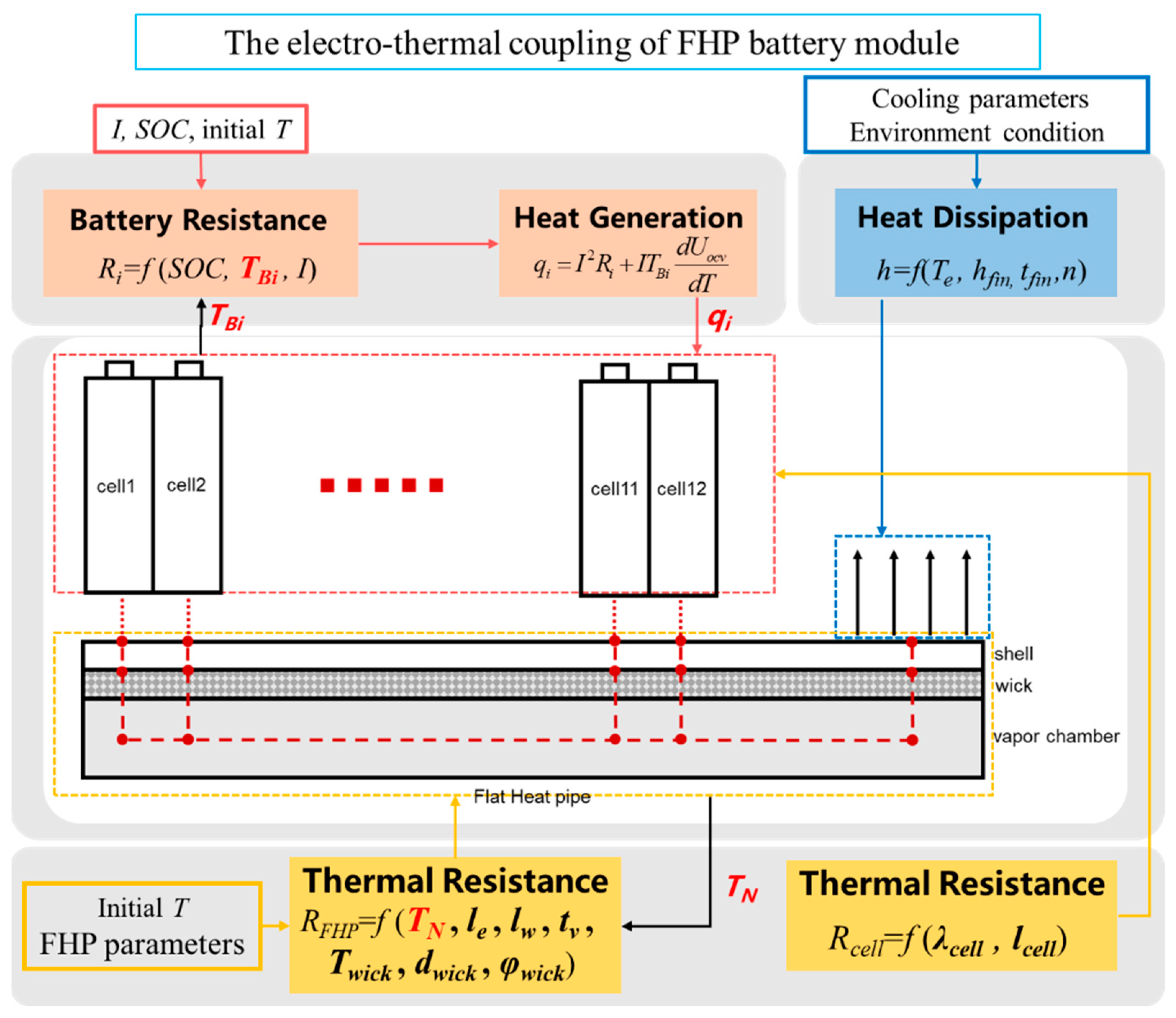
2.4. Electro-Thermal Coupled Modeling Approach

In an FHP-based BTMS, the time-varying heat generation rate is transferred into the FHP by heat conduction. After a series of heat transfer processes, the heat eventually dissipates by the cooling medium at the cooling end of the FHP. Therefore, the temperature value of each contact surface between the battery cells and the FHP can be solved through mathematical calculations. The temperature was defined as the boundary condition of batteries. The specific calculation process is presented in Figure 4. At each time step, the heat generation rate of each battery was calculated by the heat generation model and was transferred into the FHP model as the input condition. The temperature of each node was obtained by solving the energy equation for each control volume. In the meanwhile, the FHP thermal resistance, which varies with temperature, could be obtained at each time step. Through the coupling calculation mentioned above, the thermal characteristics of the BTMS could be obtained.

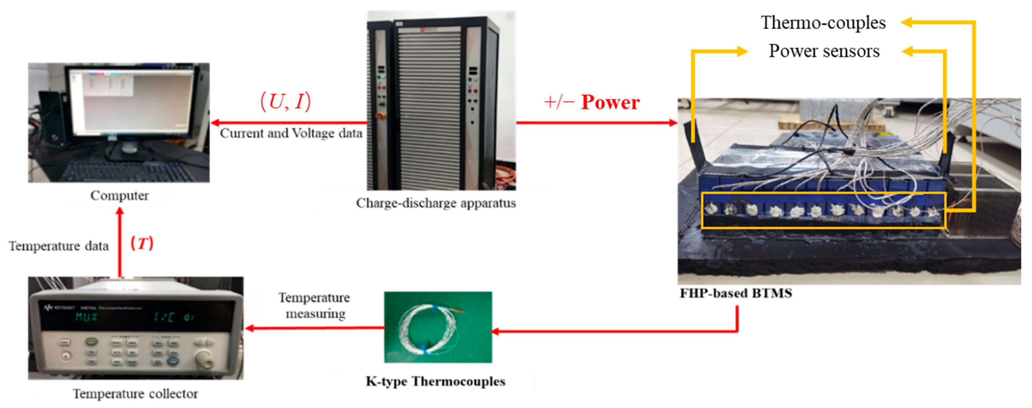
2.5. Verification of FHP-Based BTMS Thermo-Electric Coupled Model

The experimental setup is shown in Figure 5. It is mainly composed of an FHP-based BTMS, charge-discharge apparatus, a temperature collector, an industrial Personal Computer (IPC) and 24 K-type thermocouples. The BTMS includes 12 prismatic batteries and an FHP, just as in the configuration introduced in Section 2.1. The charge-discharge apparatus (Digatron EVT300-0600, Digatron, Aachen, Germany) provides operating loads and electric source. The charging and discharging procedures of the battery module are controlled by the IPC. The IPC also plays the role of electrical signal measurement and collection, whose relative uncertainty is below 0.1%. The temperature data of the batteries are collected by the data collector (Agilent 34972A, Agilent, Beijing, China) through K-type thermocouples, which have an accuracy of 0.15 + 0.002|T| °C and set the transmit frequency as 1 Hz. The thermocouples are placed at the center position on both sides of the battery, as shown in Figure 5.

The simulation results and experimental data under constant discharging current of 0.5 C, 1 C and 1.5 C are compared first. The temperature of the sixth thermocouple in Figure 6 is chosen as a representative, and the node at the same position is selected in our model. In the constant discharging case, an air-cooling velocity of 0 m·s^–1 (natural convection) and 5 m·s^–1 are adopted, and the results are shown in Figure 6a and Figure 6b, respectively. The discharging capacity is set to 80% SOC, so that the experimental times are 6400 s, 2880 s and 1920 s for 0.5 C, 1 C and 1.5 C. After every discharging process, 2–4 h is applied to the battery for relaxation. When the measuring temperature has dropped to be equal to the environment, the charging process is started up. The upper and lower cut-off voltages are set to 4.2 V and 2.7 V per cell, in case over-charging/discharging occur. Due to the random variation of the environmental temperature in different cases, temperature rise is utilized as the comparison indicator. All experiments are started with the environmental temperature around 20 °C; thus, the initial temperature of the simulation is also set to 20 °C.

From Figure 6, it can be observed that the battery temperature rise is significantly reduced when the fan is turned on. Under different discharge rates, there is good agreement between the simulations and experiments both for natural convection and forced-air cooling. The relative root mean square error (RSME) between the simulated and experimentally measured temperatures is calculated by Equation (13), and the results are shown in

Table 5. Relative RSMEs of FHP-based BTMS thermo-electric coupled model compared to experiments.

Operating Condition	0.5 C		1 C		1.5 C		WLTC
Relative RSMEs	Fan off 8.14%	Fan on 8.74%	Fan off 3.10%	Fan on 1.82%	Fan off 2.93%	Fan on 1.98%	12.38%

. It is evident that there is a relatively large discrepancy at 0.5 C. This is because during the experimental process the ambient temperature fluctuates, and at lower discharge rates the temperature is more influenced by the ambient temperature, while the simulation can only assume a constant ambient temperature.

$$\mathrm{Relative} \mathrm{RSME}=\frac{1}{N}\sqrt{{\displaystyle \sum _{i=1}^N{(\frac{T_{S,i}-T_{E,i}}{\Delta T})}^2}}$$

(13)

Then, the temperature results of the model and the experiment were compared under a cycle of the Worldwide harmonized Light vehicles Test Cycle (WLTC) condition [41]. The standard current profile for one cycle of the WLTC condition is shown in Figure 7. In this case, the ambient temperature was set to 10 °C, and the fan speed was set to 0 (natural convection) to better observe the battery temperature rise. The experimental duration was set to 1800 s, which corresponds to one WLTC cycle. Figure 8 presents the comparison of results, and the relative error between the simulation and experiment is also shown in Table 5. This indicates that the model proposed in this paper can also adapt well to dynamic current conditions.

3. Implementation of Thermal Convolution Method

Battery temperature is one of the most significant characteristics estimated by BMS algorithm. Nevertheless, the temperature information can only obtain by limited number of thermocouples in battery pack in practical. The existing control-oriented thermal models are lumped-parameter in most cases, and hardly reflect transient thermal behavior when large gradient mutation of operating current occur.

It can be observed from Equation (12) that energy conservation equation of each node in battery thermal resistance network manifests linear characteristics. Therefore, the relationship between the driving of distributed heat/cold sources and the nodes’ temperature responses can be described as a linear system. The TCRN model can be simplified by a 0-D reduced order model based on linear combination and temporal convolution of temperature response.

3.1. Temperature Response of a Particular Node inside a Battery Cell to Impulse Excitation

According to the superposability of linear systems, any input signal can be decomposed into the permutation and combination of basic signals. Using the response of the original system to these basic signals, the response to any signal can be obtained by using linear combination. For any discrete-time signal, it can be decomposed into a linear combination of weighted and temporal shifted unit impulse signals δ(t). The mathematical expression of the unit impulse signal is the Dirac function. When generating a unit impulse signal in practice, it will be more like a rectangular wave, as shown in Equation (14).

$$\delta (t)=\{\begin{array}{l}\frac{1}{h} ,0\le t\le h\\ 0 , t<0|t>h\end{array}$$

(14)

Then, we used h(n) and h(t) to represent the response of a linear system to the unit impulse signal δ(n) and δ(t) under continuous and discrete conditions, respectively. Its response to any signal is a combination of h(n) after weighting and translation, which means the system response y(n) to a discrete time signal u(n) can be expressed through linear combination of a series of delayed unit impulse responses by Equation (15). When it involves continuous time systems, y(t) can be rewritten into the integral form as shown in Equation (16), which is very similar to the formation of convolution.

Then, h(t) is used to represent the temperature response of a particular node inside No. 6 battery cell to the unit impulse heat source signal, and the temperature response to any signal is a combination of h(t) after weighting and translation. The node temperature response y(t) at time t to the heat source signal u(t) during past times can be expressed by a combination of series-delayed unit pulse responses, which is very similar to the formation of convolution.

$$\mathbf{y}(n)={\displaystyle \sum _{i=1}^n\mathbf{u}(i)\mathbf{h}(n-i)}$$

(15)

$$y(t)={\displaystyle {\int }_{-\infty }^{t}u}(\tau )h(t-\tau )d\tau$$

(16)

Hence it is reasonable to reconstruct the temperature of a particular node, which is located inside battery cell no. 6 in this paper, by means of combining different responses to various heat/cold sources. As shown in Figure 9, the FHP battery module is divided into 14 heat/cold sources. Sources 1–12 correspond to the heat generation of Cell 1-Cell 12, respectively, and can be obtained by Equation (2). Source 13 represents the natural convection between the air and the battery top surface. Source 14 is the heat sink, which represents the heat conducted from the battery bottom surface and then dissipated through convection between the fin and the forced airflow at the condensation part of the FHP. Equation (17) presents the formula of u_i(t).

$$\{\begin{array}{l}{u}_{13}(\tau )=h_{\mathrm{air}}{A}_b(T(\tau )-T_{\mathrm{air}}(\tau ))\\ u_{14}(\tau )=h_{\mathrm{fin}}{A}_f(T(\tau )-\frac{q_{FHP}{R}_{cy}}{12}-T_{cool}(\tau ))\\ u_i(\tau )=Q_i,i=\mathrm{1...12}\end{array}$$

(17)

Figure 10 shows the temperature responses of the node inside cell no. 6 to 14 sources, which are all given a rectangular pulse wave with an amplitude of 50 W and duration of 0.02 s, as an approximation of pulse excitation. What can be obviously obtained from the results is that the thermal pulse from cell no. 6 itself causes the fastest response and the highest temperature amplitude peak of the node. The thermal pulses of Cell 5 and Cell 7, which are adjacent to cell no. 6, cause the same response of overshoot but with a much smaller magnitude than cell no. 6. The thermal pulses activated by the remaining cells induce temperature responses without overshoot, due to their distant position relative to cell no. 6. As for thermal pulses from natural convection and the heat sink, the responses to these possess a similar curve but a much smaller amplitude. This is because both thermal impulses are divided equally between each cell almost at the same moment.

Finally, the temperature responses eventually tend to a state approaching thermal equilibrium. The same heat balance temperature is represented in Figure 10, which is in accord with the result of steady-state energy conservation. It can be further observed from the figure that the temperature responses of the node to thermal pulses generally take close to 600 s before reaching equilibrium, due to the heat transfer architecture of the battery module and the combined thermal mass. Meanwhile, each battery cell is affected by its own and external thermal excitation at every moment, which means a cell itself could not reach a state of thermal balance throughout its working period. In this case, the potential temperature overshoot cannot be identified by a steady-state method assuming thermal equilibrium. When the instantaneous discharge C-rate increases/decreases suddenly, predictably, the temperature prediction based on the lumped control model may exhibit poor tracking behavior and cause more risk. The relevant research work will be introduced in the next section.

Before that, it is necessary to make corrections to the heat dissipation of the FHP-BTMS in order to improve the accuracy of the estimated q14 in the thermal convolution method. Therefore, the thermal convolution method for a given node is as follows in Equation (18): the current temperature of the node can be obtained using past thermal/cold source boundary conditions and the pulse response characteristics. To achieve a prediction, Equation (18) needs to be extended in the time domain, as shown in Equation (19), by adding future K-time operating condition inputs to determine the future effects of heat sources and cold sources on the node.

$$T(t)={\displaystyle {\sum }_{i=1}^N{\displaystyle {\int }_{-\infty }^t{u}_i}(\tau )h_i(t-\tau )d\tau }$$

(18)

$$T(t+K)={\displaystyle {\sum }_{i=1}^N{\displaystyle {\int }_{-\infty }^{t+K}{u}_i}(\tau )h_i(t-\tau )d\tau }$$

(19)

3.2. Correction of the Heat Flux throughout the FHP

Unlike traditional air-cooled and liquid-cooled BTMSs, the dissipation heat flow throughout a FHP-based BTMS is closely related to the dynamic heat transfer characteristics of the flat heat pipe.

As the temperatures of the evaporator and condenser sections change, the mass flow rate of the liquid working fluid from the wick evaporating into the vapor chamber also changes. This can be intuitively expressed as the heat dissipation of the FHP to the battery module dynamically changing when the battery module or cooling conditions vary. Therefore, it is necessary to modify the q_FHP term in Equation (17) to account for the dynamic thermal characteristics of the FHP. Mathematical models for the heating and cooling dynamic processes of flat plate heat pipes have been established in the literature and experimentally validated [42,43].

For the FHP described in this paper, based on a digital prototype, the multi-heat source TCRN model has been validated. The dynamic characteristics of the heat-up and cool-down processes have been investigated under different evaporator input power and condenser heat dissipation airflow, and the applicability of the model has been verified under various operating conditions such as continuous loading and unloading.

A dynamic model for the flat plate heat pipe has been established, and its formula is expressed as follows:

$$X(t)=X_{ss}(1-e^{(t_0-t)/{\tau }_h})$$

(20)

$$X(t)=X_{ss}{e}^{(t_0-t)/{\tau }_h}$$

(21)

$$\tau =\left|X_{ss}/[{(\mathrm{d}X/\mathrm{d}t)}_{t=t_0}]\right|$$

(22)

where X represents the state parameters such as heat flux and τ represents the characteristic time.

The characteristic times corresponding to different operating conditions are shown in Figure 11 below. From Figure 11a, we can observe that as the input heat power increases, both the heat-up time constants and the cool-down time constants decrease to a certain extent, but they remain within a small range, and the cool-down time constants are slightly greater than the heat-up time constants. As shown in Figure 11b, with the increasing of heat dissipation airflow rates, the time constants shows a pattern of rapid decrease followed by a tendency to level off, and there is no significant difference between the cool-down time constants and the heat-up time constants.

Based on the previous results, the interpolation model between the characteristic time constants and the cooling airflow and input heat power have been obtained. Furthermore, a dynamic model for the FHP under continuous dynamic operating conditions has been developed. Here is the expression for the flat heat pipe dynamic model (FHP-DM):

$$X^{(t)}=X^{(t-1)}\cdot (1-e^{-1/\tau (t)})+{\displaystyle \sum _{i=1}^t{X}_i}{e}^{(i-t)/{\tau }_i}$$

(23)

Figure 12 demonstrates the comparison between the dynamic model and the TCRN of the FHP for different input heat power levels. It appears that the flat plate heat pipe requires a certain time to reach its maximum heat transfer rate. The fit between the dynamic model and the TCRN indicates that the dynamic model based on thermal time constants can effectively reflect the dynamic thermal characteristics of the flat plate heat pipe during startup and shutdown processes.

Furthermore, Figure 13 illustrates the comparison between the dynamic model and the TCRN of the FHP under dynamic validation conditions, such as 200 s with a power change from 12 W to 8 W and 50 s with a power change from 12 W to 0 W. The almost identical results suggest that the dynamic model of the FHP can adequately reflect the heat transfer performance of the flat plate heat pipe under continuous loading and non-steady operating conditions.

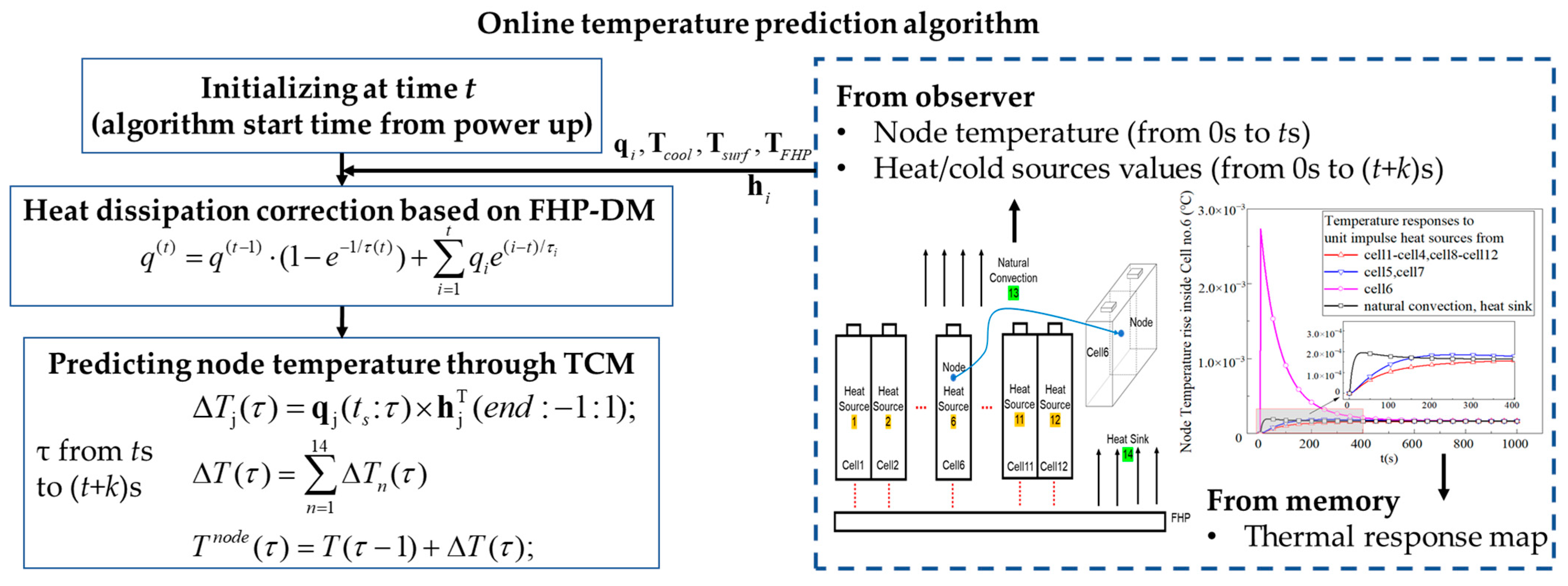
3.3. Implementation Procedure of Online Temperature Prediction Based on the TCM

The quick temperature prediction algorithm based on the thermal convolution method is summarized in the following flow chart, shown in Figure 14.

The first step is program initialization at time t, which is calculated from the beginning of the discharge process. As the experiments are based on a virtual prototype, we can obtain the current temperature of the node TCRN by utilizing an observer. The battery’s heat generation rates, q1–q12, can be determined based on the present operating current. Through the observer, we can acquire the temperatures at the condensation section of the FHP and on the battery surface, as well as the ambient temperature and cooling air temperature. Plugging these values into Equations (10) and (11) enables us to calculate the current heat transfer through natural convection and the instantaneous heat dissipation of the FHP, which are represented as q13 and q14. In order to reduce the computational cost and space occupation of the algorithm, 600 s (600 time steps) is adopted as the memory limit for thermal excitation, since it can be assumed that the temperature will not change after 600 s according to Figure 10. Consequently, the thermal response map can be reduced in row count, resulting in decreased computational load.

The second step is storing the heat source information obtained at time t in the heat source memory. Additionally, we adjust the heat dissipation of the FHP based on the operational corrections outlined in Section 3.2.

In the third step, the temperature trend of the nodes for the next k seconds is predicted. This involves the implementation of two nested loops. The outer loop iterates from the current time to the prediction termination time, while the inner loop performs matrix operations for the 14 heat sources. Referring to the explanation in Section 3.1, the product of the heat source q and the inverse response function h in the time domain yields the temperature rise at the current time step. By summing the results obtained from the inner loop, the temperature at the current time can be determined. Once the outer loop concludes, the temperature variations of the nodes from time t to t + k can be obtained.

To evaluate the computational speed and memory usage of the temperature prediction algorithm, comparative analysis on a computer with an R7-4800H CPU was conducted. We compared the performance of the lumped model, the TCRN and the algorithm based on the TCM with a temperature-predicting period of 600 s. The results, as presented in

Table 6. CPU-time comparison between the TCM, the lumped model and the TCRN.

	TCM	Lumped Model	TCRN
CPU-time	47 ms	5 ms	26.81 s

, indicate that while the TCM exhibits higher computational speed and memory consumption compared to the lumped model, it still can meet the requirements of making real-time predictions.

4. Results and Discussion

In this section, specific examples are presented to compare and analyze the temperature prediction precision, operational adaptability and stability of the TCM and the lumped model. Figure 15a–e illustrates dynamic scenarios where the battery is discharged continuously from 1 C to 5 C for 120 s at an initial temperature of 20 °C and suddenly terminated. The condensation section fan of the FHP remains off, allowing for natural cooling. Apart from the numerical values of temperature rise, the five figures exhibit good consistency in terms of patterns. It is observed that the surface temperature of the battery responds to changes in operational conditions with a delay of approximately 30 s compared to the internal temperature of the battery. The temperature prediction algorithm based on the TCM can consistently track the dynamic temperature changes during the entire period in response to varying operational conditions. On the other hand, although the lumped model can provide timely responses to dynamic operational changes, it struggles to reflect the current temperature distribution within the battery. As the discharge rate increases, the absolute deviation of temperature predicted by the lumped model becomes larger. The relative errors and maximum absolute temperature deviations in temperature prediction by the TCM and the lumped model under different shutdown conditions are shown in

Table 7. Relative error (RE) and maximum absolute error (MAE) of the TCM and the lumped model under different dynamic conditions.

		TCM		Lumped Model
		RE	MAE	RE	MAE
Dynamic current	1 C	2.20%	0.01 °C	12.70%	0.07 °C
	2 C	2.20%	0.06 °C	12.69%	0.28 °C
	3 C	2.19%	0.12 °C	12.67%	0.62 °C
	4 C	2.18%	0.21 °C	12.64%	1.04 °C
	5 C	2.18%	0.31 °C	12.61%	1.55 °C
	Step	6.24%	1.27 °C	45.06%	10.39 °C
Dynamic air velocity	1 C	26.12%	0.13 °C	141.45%	0.84 °C
	2 C	7.37%	0.33 °C	92.29%	1.50 °C
	3 C	6.54%	0.60 °C	25.02%	2.32 °C
	4 C	6.23%	0.98 °C	23.39%	3.46 °C
	5 C	6.10%	1.43 °C	22.64%	4.80 °C
Dynamic air temperature	1 C	34.24%	0.14 °C	175.90%	0.83 °C
	2 C	7.66%	0.31 °C	28.04%	1.37 °C
	3 C	6.40%	0.61 °C	22.56%	2.19 °C
	4 C	6.02%	0.99 °C	20.82%	3.23 °C
	5 C	5.85%	1.44 °C	20.02%	4.46 °C

. The TCM achieves an overall accuracy improvement of 83% compared to the lumped model.

Figure 16 presents a comparison between the TCM and the lumped model under a step change scenario, with a discharge rate ranging from 1 C to 5 C. It is evident that the appearance of inflection points in surface temperature consistently lags behind the operational changes. Moreover, as time progresses, the relative errors in temperature prediction increase. The TCM manages to maintain a relative error of 6.24% even under such continuously changing operational conditions.

Next, comparisons of the accuracy and adaptability of the TCM and the lumped model are conducted under dynamic cooling conditions with sudden changes in operational scenarios. Figure 17a–e represents a constant current ranging from 1 C to 5 C. In these scenarios, the fan located at the condensation section of the FHP remains off for the first 120 s and then switches on at 120 s with a flow rate of 0.098 kg/s, corresponding to an airflow velocity of 10 m/s. The cooling air temperature is set to 10 °C. It can be observed that in the 1 C and 2 C scenarios, inflection points in surface temperature and internal temperature change lines can be obviously detected. Due to the dynamic response characteristics of the FHP and battery module, there is a delay before the internal temperature begins to decrease after the surface temperature starts to decline. For discharge currents of 3 C and above, the inflection points caused by sudden cooling condition changes are less noticeable. This is due to the limited heat transfer coefficient of the air cooling, resulting in insufficient cooling capacity of the FHP. This phenomenon also indicates that the heat transfer capacity of the heat pipe, when applied to a BTMS, is actually limited by the cooling capacity at the cold end. Sometimes, there can be a situation where the heat transfer capacity of the heat pipe far exceeds the cooling capacity at the cold end, resulting in poor heat dissipation. The TCM demonstrates better performance in following the internal temperature under different discharge rates compared to the lumped model. Since the lumped model does not consider the dynamic heat transfer performance of the FHP, it leads to significant errors in estimating the cooling capacity of the battery module after sudden changes in cooling conditions. This is also the reason behind the rapid temperature drop observed in the lumped model after operational changes. Figure 17a–e represents constant current scenarios from 1 C to 5 C, with the FHP condensation section fan continuously operating at a fixed airflow velocity of 10 m/s. However, at 120 s, the cooling air temperature suddenly changes from 20 °C to 10 °C. The patterns observed in these figures are similar to those in Figure 18.

Table 7 provides the average prediction accuracy and absolute prediction deviation of the TCM and the lumped model under different conditions. The TCM consistently outperforms the lumped model by 70–80% in terms of accuracy.

The high discharge rate dynamic current profile is derived from the research on VTOL flight missions of flying cars, as mentioned in reference [43]. In this case, the current profile, cooling airflow velocity and temperature are provided to compare the temperature prediction performance of the lumped model and the TCM. The results and relative errors are shown in Figure 19 and Figure 20, respectively. It can be observed that the TCM consistently exhibits higher temperature accuracy than the lumped model throughout the entire prediction time domain. The temperature prediction error of the TCM remains within 5%. On the other hand, the temperature prediction accuracy of the lumped model decreases over time, possibly due to accumulated errors. Considering the previous studies, the TCM can be considered as an effective approach for online battery temperature prediction in a BTMS. When combined with corresponding prediction controllers, it enables more accurate and convenient achievement of control objectives such as thermal management energy optimization and battery temperature regulation.

5. Conclusions

This paper focuses on the challenge of accurately predicting the temperature variation of batteries for a FHP-BTMS under dynamic operating and boundary conditions. A quick temperature prediction algorithm based on the TCM, considering the dynamic thermal characteristics of FHP-BTMSs, is developed. By comparing with the simulation platform based on a TCRN, the temperature prediction accuracy and adaptability of the lumped model and the TCM under different dynamic conditions are analyzed. The main conclusions are as follows:

(1) The relative RSMEs between the TCRN of an FHP-based BTMS and experimental data under constant C-rates and the WLTC profile validates the thermo-electrical modeling and the accuracy of the simulation platform;

(2) With a prediction time domain of 600 s, the temperature-predicting algorithm based on the TCM has a runtime of 47 ms. Although longer than the lumped model, it still can meet the computational requirements and limitations for fast calculation for real-time prediction;

(3) In the study of dynamic current, for sudden shutdown scenarios, the TCM achieves a relative error of 2.2% for discharge rates ranging from 1 C to 5 C. For long-duration step-type current scenarios, the error is still only 6.24%. In dynamic cooling conditions, the TCM can effectively track the temperature variations of nodes with changes in cooling airflow velocity or cooling airflow temperature. With the benefit of heat dissipation rate correction, it exhibits significantly higher temperature prediction accuracy and 70–80% improvement compared to the lumped model, with an absolute temperature error of 1.5 °C. Under the VTOL mission profile, the TCM maintains its superior dynamic tracking performance and achieves a prediction accuracy of within 5% throughout the 870 s prediction time domain.

The key focus of the TCM lies in obtaining the temperature response map of nodes under different thermal excitations. In this paper, the map was obtained from a validated digital prototype. However, these temperature response curves can also be obtained from real experimental tests and then calibrated. Therefore, this method has good practicality and applicability, with broad prospects for applications in BMS temperature prediction and global optimal control strategy design.

References

1. Sharmili, N.; Nagi, R.; Wang, P. A review of research in the Li-ion battery production and reverse supply chains. J. Energy Storage 2023, 68, 107622. [Google Scholar] [CrossRef]
2. Zhou, H.; Zhou, F.; Xu, L.; Kong, J.; Yang, Q. Thermal performance of cylindrical Lithium-ion battery thermal management system based on air distribution pipe. Int. J. Heat Mass Transf. 2018, 131, 984–998. [Google Scholar] [CrossRef]
3. Das, D.; Manna, S.; Puravankara, S. Electrolytes, Additives and Binders for NMC Cathodes in Li-Ion Batteries—A Review. Batteries 2023, 9, 193. [Google Scholar] [CrossRef]
4. Wu, S.; Wang, C.; Luan, W.; Zhang, Y.; Chen, Y.; Chen, H. Thermal runaway behaviors of Li-ion batteries after low temperature aging: Experimental study and predictive modeling. J. Energy Storage 2023, 66, 107451. [Google Scholar] [CrossRef]
5. Shahjalal, M.; Shams, T.; Islam, E.; Alam, W.; Modak, M.; Bin Hossain, S.; Ramadesigan, V.; Ahmed, R.; Ahmed, H.; Iqbal, A. A review of thermal management for Li-ion batteries: Prospects, challenges, and issues. J. Energy Storage 2021, 39, 102518. [Google Scholar] [CrossRef]
6. Kumar, R.; Goel, V. A study on thermal management system of lithium-ion batteries for electrical vehicles: A critical review. J. Energy Storage 2023, 71, 108025. [Google Scholar] [CrossRef]
7. Li, W.; Garg, A.; Xiao, M.; Gao, L. Optimization for Liquid Cooling Cylindrical Battery Thermal Management System Based on Gaussian Process Model. J. Therm. Sci. Eng. Appl. 2021, 13, 1–19. [Google Scholar] [CrossRef]
8. He, F.; Ma, L. Thermal management of batteries employing active temperature control and reciprocating cooling flow. Int. J. Heat Mass Transf. 2015, 83, 164–172. [Google Scholar] [CrossRef]
9. Behi, H.; Karimi, D.; Behi, M.; Jaguemont, J.; Ghanbarpour, M.; Behnia, M.; Berecibar, M.; Van Mierlo, J. Thermal management analysis using heat pipe in the high current discharging of lithium-ion battery in electric vehicles. J. Energy Storage 2020, 32, 101893. [Google Scholar] [CrossRef]
10. Smith, J.; Singh, R.; Hinterberger, M.; Mochizuki, M. Battery thermal management system for electric vehicle using heat pipes. Int. J. Therm. Sci. 2018, 134, 517–529. [Google Scholar] [CrossRef]
11. Yu, Z.; Zhang, J.; Pan, W. A review of battery thermal management systems about heat pipe and phase change materials. J. Energy Storage 2023, 62, 106827. [Google Scholar] [CrossRef]
12. Zhang, Z.; Wei, K. Experimental and numerical study of a passive thermal management system using flat heat pipes for lithium-ion batteries. Appl. Therm. Eng. 2020, 166, 114660. [Google Scholar] [CrossRef]
13. Jouhara, H.; Serey, N.; Khordehgah, N.; Bennett, R.; Almahmoud, S.; Lester, S.P. Investigation, development and experimental analyses of a heat pipe based battery thermal management system. Int. J. Thermofluids 2019, 1, 100004. [Google Scholar] [CrossRef]
14. Liu, W.; Jia, Z.; Luo, Y.; Xie, W.; Deng, T. Experimental investigation on thermal management of cylindrical Li-ion battery pack based on vapor chamber combined with fin structure. Appl. Therm. Eng. 2020, 162, 114272. [Google Scholar] [CrossRef]
15. Mei, N.; Xu, X.; Li, R. Heat Dissipation Analysis on the Liquid Cooling System Coupled with a Flat Heat Pipe of a Lithium-Ion Battery. ACS Omega 2020, 5, 17431–17441. [Google Scholar] [CrossRef]
16. Mo, X.; Hu, X.; Tang, J.; Tian, H. A comprehensive investigation on thermal management of large-capacity pouch cell using micro heat pipe array. Int. J. Energy Res. 2019, 43, 7444–7458. [Google Scholar] [CrossRef]
17. Gan, Y.; He, L.; Liang, J.; Tan, M.; Xiong, T.; Li, Y. A numerical study on the performance of a thermal management system for a battery pack with cylindrical cells based on heat pipes. Appl. Therm. Eng. 2020, 179, 115740. [Google Scholar] [CrossRef]
18. Cen, J.; Jiang, F. Li-ion power battery temperature control by a battery thermal management and vehicle cabin air conditioning integrated system. Energy Sustain. Dev. 2020, 57, 141–148. [Google Scholar] [CrossRef]
19. Min, H.; Zhang, Z.; Sun, W.; Min, Z.; Yu, Y.; Wang, B. A thermal management system control strategy for electric vehicles under low-temperature driving conditions considering battery lifetime. Appl. Therm. Eng. 2020, 181, 115944. [Google Scholar] [CrossRef]
20. Gao, X.; Ma, Y.; Chen, H. Active Thermal Control of a Battery Pack Under Elevated Temperatures. IFAC PapersOnLine 2018, 51, 262–267. [Google Scholar] [CrossRef]
21. Lee, S.-J.; Lee, C.-Y.; Chung, M.-Y.; Chen, Y.-H.; Han, K.-C.; Liu, C.-K.; Yu, W.-C.; Chang, Y.-M. Lithium-ion Battery Module Temperature Monitoring by Using Planer Home-Made Micro Thermocouples. Int. J. Electrochem. Sci. 2013, 8, 4131–4141. [Google Scholar] [CrossRef]
22. Sun, J.; Wei, G.; Pei, L.; Lu, R.; Song, K.; Wu, C.; Zhu, C. Online Internal Temperature Estimation for Lithium-Ion Batteries Based on Kalman Filter. Energies 2015, 8, 4400–4415. [Google Scholar] [CrossRef]
23. Zhang, C.; Li, K.; Deng, J. Real-time estimation of battery internal temperature based on a simplified thermoelectric model. J. Power Sources 2016, 302, 146–154. [Google Scholar] [CrossRef]
24. Kim, Y.; Mohan, S.; Siegel, J.B.; Stefanopoulou, A.G.; Ding, Y. The Estimation of Temperature Distribution in Cylindrical Battery Cells Under Unknown Cooling Conditions. IEEE Trans. Control. Syst. Technol. 2014, 22, 2277–2286. [Google Scholar] [CrossRef]
25. Li, W.; Xie, Y.; Hu, X.; Zhang, Y.; Li, H.; Lin, X. An Online SOC-SOTD Joint Estimation Algorithm for Pouch Li-Ion Batteries Based on Spatio-Temporal Coupling Correction Method. IEEE Trans. Power Electron. 2021, 37, 7370–7386. [Google Scholar] [CrossRef]
26. Hu, X.; Asgari, S.; Yavuz, I.; Stanton, S.; Hsu, C.-C.; Shi, Z.; Wang, B.; Chu, H.-K. A Transient Reduced Order Model for Battery Thermal Management Based on Singular Value Decomposition. In Proceedings of the 2014 IEEE Energy Conversion Congress and Exposition (ECCE), Pittsburgh, PA, USA, 14–18 September 2014; pp. 3971–3976. [Google Scholar]
27. Asgari, S.; Hu, X.; Tsuk, M.; Kaushik, S. Application of POD plus LTI ROM to Battery Thermal Modeling: SISO Case. SAE Int. J. Commer. Veh. 2014, 7, 278–285. [Google Scholar] [CrossRef]
28. Kleiner, J.; Stuckenberger, M.; Komsiyska, L.; Endisch, C. Real-time core temperature prediction of prismatic automotive lithium-ion battery cells based on artificial neural networks. J. Energy Storage 2021, 39, 102588. [Google Scholar] [CrossRef]
29. Wang, Y.; Xiong, C.; Wang, Y.; Xu, P.; Ju, C.; Shi, J.; Yang, G.; Chu, J. Temperature state prediction for lithium-ion batteries based on improved physics informed neural networks. J. Energy Storage 2023, 73, 108863. [Google Scholar] [CrossRef]
30. Al Miaari, A.; Ali, H.M. Batteries temperature prediction and thermal management using machine learning: An overview. Energy Rep. 2023, 10, 2277–2305. [Google Scholar] [CrossRef]
31. Zhang, W.; Wan, W.; Wu, W.; Zhang, Z.; Qi, X. Internal temperature prediction model of the cylindrical lithium-ion battery under different cooling modes. Appl. Therm. Eng. 2022, 212, 118562. [Google Scholar] [CrossRef]
32. Dan, D.; Li, W.; Zhang, Y.; Xie, Y. A quasi-dynamic model and thermal analysis for vapor chambers with multiple heat sources based on thermal resistance network model. Case Stud. Therm. Eng. 2022, 35, 102110. [Google Scholar] [CrossRef]
33. Jiang, Y.; Carbajal, G.; Sobhan, C.B.; Li, J. 3D Heat Transfer Analysis of a Miniature Copper-Water Vapor Chamber with Wicked Pillars Array. ISRN Mech. Eng. 2013, 2013, 194908. [Google Scholar] [CrossRef]
34. Patankar, G.; Weibel, J.A.; Garimella, S.V. On the transient thermal response of thin vapor chamber heat spreaders: Optimized design and fluid selection. Int. J. Heat Mass Transf. 2020, 148, 119106. [Google Scholar] [CrossRef]
35. Thomas, K.E.; Newman, J. Thermal Modeling of Porous Insertion Electrodes. J. Electrochem. Soc. 2003, 150, A176–A192. [Google Scholar] [CrossRef]
36. Singh, R.; Akbarzadeh, A.; Mochizuki, M. Effect of Wick Characteristics on the Thermal Performance of the Miniature Loop Heat Pipe. J. Heat Transf. 2009, 131, 082601. [Google Scholar] [CrossRef]
37. Liu, F.; Lan, F.; Chen, J. Dynamic thermal characteristics of heat pipe via segmented thermal resistance model for electric vehicle battery cooling. J. Power Sources 2016, 321, 57–70. [Google Scholar] [CrossRef]
38. Bergman, T.L.; Lavine, A.S.; Incropera, F.P.; DeWitt, D.P. Fundamentals of Heat and Mass Transfer; John Wiley & Sons: New York, NY, USA, 2015; Volume 13. [Google Scholar]
39. Ranjan, R.; Murthy, J.Y.; Garimella, S.V.; Vadakkan, U. A numerical model for transport in flat heat pipes considering wick microstructure effects. Int. J. Heat Mass Transf. 2011, 54, 153–168. [Google Scholar] [CrossRef]
40. Tutuianu, M.; Bonnel, P.; Ciuffo, B.; Haniu, T.; Ichikawa, N.; Marotta, A.; Pavlovic, J.; Steven, H. Development of the World-wide harmonized Light duty Test Cycle (WLTC) and a possible pathway for its introduction in the European legislation. Transp. Res. Part D Transp. Environ. 2015, 40, 61–75. [Google Scholar] [CrossRef]
41. El-Genk, M.S.; Lianmin, H. An experimental investigation of the transient response of a water heat pipe. Int. J. Heat Mass Transf. 1993, 36, 3823–3830. [Google Scholar] [CrossRef]
42. Chang, W.S.; Colwell, G.T. Mathematical Modeling of The Transient Operating Characteristics of a Low-Temperature Heat Pipe. Numer. Heat Transf. 1985, 8, 169–186. [Google Scholar] [CrossRef]
43. Luo, Y.; Qian, Y.; Zeng, Z.; Zhang, Y. Simulation and analysis of operating characteristics of power battery for flying car utilization. eTransportation 2021, 8, 100111. [Google Scholar] [CrossRef]
Figure 1. Schematic of an FHP-based BTMS of 12 cells and working principle of the FHP [32].
Batteries 10 00019 g001
Figure 2. HPPC internal resistance testing process.
Batteries 10 00019 g002
Figure 3. Thermal network topology of the FHP-based BTMS.
Batteries 10 00019 g003
Figure 4. The electro-thermal coupling model of the FHP battery module.
Batteries 10 00019 g004
Figure 5. Schematic representation of the experimental system devices.
Batteries 10 00019 g005
Figure 6. Comparison of experiments and simulation under constant discharging current: (a) FHP with natural convection, (b) FHP with air cooling.
Batteries 10 00019 g006
Figure 7. WLTC Discharging Current Profile.
Batteries 10 00019 g007
Figure 8. Comparison of experiments and simulation under the WLTC profile.
Batteries 10 00019 g008
Figure 9. The location of 14 variable heat/cold sources.
Batteries 10 00019 g009
Figure 10. Temperature response hi(t) of node inside cell no. 6 to different unit pulse heat sources.
Batteries 10 00019 g010
Figure 11. Heat-up and cool-down time constants variation with (a) power input and (b) airflow rate.
Batteries 10 00019 g011
Figure 12. Comparison between the TCRN and the FHP-DM under different heat input and shut-down conditions.
Batteries 10 00019 g012
Figure 13. Comparison between the FHP-TCRN model and the FHP-DM. (a) Continuous power input 12 W(200 s)–8 W, (b) Continuous power input 12 W(50 s)–0 W.
Batteries 10 00019 g013
Figure 14. Flow chart of quick temperature prediction algorithm based on the thermal convolution method.
Batteries 10 00019 g014
Figure 15. Results comparison of the lumped model, the TCM, battery surface temperature, battery core temperature: (a) 1 C-break condition; (b) 2 C-break condition; (c) 3 C-break condition; (d) 4 C-break condition; (e) 5 C-break condition.
Batteries 10 00019 g015
Figure 16. Step-loading condition.
Batteries 10 00019 g016
Figure 17. Temperature prediction comparison between the lumped model and the TCM under (a) 1C, (b) 2C, (c) 3C, (d) 4C, (e) 5C conditions, when the fan starts at 120 s and the temperature of cooling air is set to 10 °C.
Batteries 10 00019 g017
Figure 18. Temperature prediction comparison between the lumped model and the TCM under (a) 1C, (b) 2C, (c) 3C, (d) 4C, (e) 5C condition, when the temperature of cooling air changes from 20 °C to 10 °C at 120 s.
Batteries 10 00019 g018
Figure 19. Results of the lumped model, the TCM, battery surface temperature and core temperature (under VTOL mission profile).
Batteries 10 00019 g019
Figure 20. Relative error of the lumped model, the TCM and battery surface temperature.
Batteries 10 00019 g020