Abstract
The effect of structural relaxations on the magnetocrystalline anisotropy energy (MAE) was investigated by using density functional theory (DFT). The theory of the impact of magnetostructural coupling on the MAE was discussed, including the effects on attempt frequency. The MAE for ferromagnetic FePt (3.45 meV/formula unit) and antiferromagnetic PtMn (0.41 meV/formula unit) were calculated within the local density approximation (LDA). The effects of the structural relaxation were calculated and found to give a <0.5% reduction to the MAE for the ferromagnet and ∼20% for the antiferromagnet.
1. Introduction
The modern world has been transformed since the advent of the computer due to ever-improving data storage, enabling more complex devices and programmes to be manufactured and written. Huge advances have been made possible due to the development of and improvements in magnetic data storage from the primitive core-rope memory (∼4 Kb) of the Apollo era [1], to modern multi-Tb storage drives [2]. This progress has depended upon the construction of an ever-greater areal bit density (number of data storage "sites" per unit area) [2] and higher performance bits.
For high performance (high clock speed) memory, such as is found in modern random access memory (RAM), the storage must typically be electric rather than magnetic, because conventional magnetic storage techniques take too long to write a bit. This causes the memory to be volatile [3], and has a sizable effect on the power consumption of that memory, because constant refreshing of the bits is required. One potential way around this is antiferromagnetic magnetoelectric RAM (AFM-MERAM) [4], which makes use of the high-switching speeds of antiferromagnetic (AFM) materials to create memory that offers equivalent performance to standard charge-based RAM while still having the low energy requirements and nonvolatility of magnetic storage.
Now, considering the areal bit density, the greatest current limit is the requirement that the memory itself is thermally stable [5]; it is not much use if a warm day causes the data to be erased due to random bits flipping. Therefore, it is necessary to have a high barrier against bit-flipping, such that the probability of a random flip caused by thermal fluctuations is very small, even over long timescales (there must be a high activation energy for the bit flipping at for typical operational temperatures).
In modern memory-storage devices that rely upon the magnetisation orientation of a magnetic material, this barrier to bit flipping is controlled by the energy required to reorient all of the spin moments within the bit. This barrier is therefore extrinsic, and increases with the size of the device. Any increase of the areal bit density, however, requires shrinking the size of a bit, and therefore to maintain a constant barrier to flipping needs a higher intrinsic barrier to flipping.
This intrinsic barrier to the flipping of individual bits is the magnetocrystalline anisotropy. This property, typically evaluated as a magnetocrystalline anisotropy energy (MAE), is a relativistic effect induced by spin-orbit coupling linking together orbital and spin angular momenta. One way of thinking about this effect is that, in the absence of relativity, spins exist in a spherical orbital. This may then be convolved with an electronic orbital to produce the standard “spin-orbitals” of, for example, Hartree–Fock theory, without affecting the spins. In the relativistic limit, however, l and s are no longer acceptable quantum numbers, and therefore we cannot neglect the effect of the convolution on the spin-like degrees of freedom. Because the original electronic orbitals are both directionally dependent and oriented with respect to the crystal lattice (due to the crystal field effect), this means that the effect of spin-orbit coupling is to make the spins experience an environment which is directionally dependent — magnetocrystalline anisotropy.
Much effort has gone into evaluating MAE over the years, both in ferromagnetic (FM) and antiferromagnetic (AFM) materials through both experimental [6,7] and theoretical [8,9,10] approaches based on ab initio calculation. For antiferromagnetic materials in particular, this is made especially difficult by their lack of apparent response to an applied field, and therefore the MAE of AFM materials tends to be inferred rather than directly measured [7].
Reliable simulation techniques have huge potential within the field of materials discovery because they enable a cheap initial search of likely candidate materials and novel structures [11,12], which may then be synthesised to confirm the findings of the simulations. For AFM materials in particular, in which the MAE is not directly accessible, this ability to directly access a magnetic property through a simulation is a potentially important avenue for materials discovery. Current simulation methods, however, typically significantly overestimate the anisotropy value compared with experiment [8,9].
One reason for this discrepancy between theory and experiment may be that the theoretical simulations do not calculate precisely the same observable that is measured experimentally, such as different timescales of experiment and theory. This sort of error cannot be corrected by using more sophisticated treatments of the electronic structure — such as additional treatments of strong correlations, or better exchange-correlation functionals — because these better methods for electronic structure would still be applied toward more accurately calculating the wrong number. Additionally, by finding a more experimentally relevant description it is possible to gain greater insight into the underlying physical processes, thereby both enhancing understanding and potentially opening up new routes for device optimisation and material parameters tuning.
A potential cause of the overestimation of MAE may be that these techniques typically rely on optimising the ground-state structure and then either sampling different constrained spin orientations [13] or calculating the spin-torque and using that to evaluate the anisotropy [14]. These methods, however, do not typically allow for a relaxation of the crystal structure in response to the changing spin orientation. In this paper, we propose a new strategy to evaluate the magnetic anisotropy which also includes the magnetostructural coupling and apply these to ferromagnetic FePt and antiferromagnetic PtMn.
2. Theory
2.1. Magnetic Transition State Searching
Rather than the narrow definition of MAE as the difference in energy between orientation of the spins along the magnetic easy and hard axes, it is possible to extend the definition to a higher dimensional case (i.e., also considering structural relaxations) by instead defining it as the maximum energy of the minimum energy pathway — the energy of the transition state — between the magnetic ground state and its symmetrically identical reversed state (for example turning all "up" spins into "down" spins and vice versa). When we only consider magnetic relaxations, this definition yields the same MAE as before. However, when simultaneous structural and magnetic relaxations are considered (as must be the case in a real experiment) the extra degrees of freedom make further, potentially lower, energy routes valid.
Transition state searching within chemistry, which considers only the movement of atoms, is a well-established field with many techniques for evaluating the energy barrier for transition between two local minima within a wider energy landscape (in chemical contexts, these are the reactant and product of a reaction step). Much work has been done on developing procedures for these, such as the nudged elastic band method [15,16]. However, an older, and more computationally efficient, method — known as linear synchronous transit/quadratic synchronous transit [17] (LST/QST) — may be sufficient for accurate magnetic transition state searching, and so it is used here.
In LST/QST, a linear pathway between the two minima is constructed by interpolation, and the maximum along this pathway is found through a bisection search as a first approximation to the transition state (this is the LST component). Because this state has no obligation to be a saddle point — which all transition states must be [18] — a further optimisation in directions orthogonal to the original search direction is performed until a minimum is found (the QST component). By identifying a maximum in the direction between minima which is a minimum in all other directions, the saddle point associated with the transition between local minima will have been identified.
For magnetic systems, we may consider the spin orientation of the system to be an orthogonal search direction to the structural configuration of the system (see Figure 1), because any spin configuration and any structural configuration may coexist (even if with a significant energy penalty). This suggests that performing an LST search in spin space, followed by a structural optimisation under the constraint of fixed spin orientations (in the manner of the QST component of the search) would lead to an improved estimation of the transition state. This QST style search also has benefits over standard structural-only LST/QST in that the QST relaxation is guaranteed as the constrained spin orientation cannot be altered by the change of atomic positions or lattice vectors. It is this QST-like optimisation of the crystal structure that we propose as a necessary minimum correction to evaluate the true transition state between two magnetic configurations (a more sophisticated evaluation of the transition state would require a more sophisticated technique).
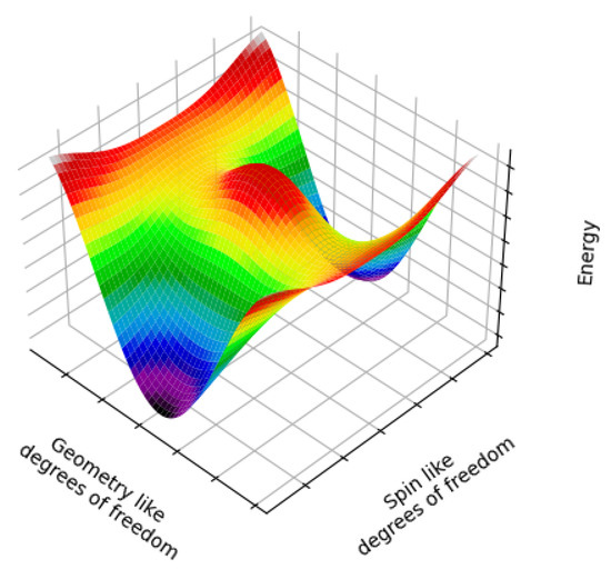
Figure 1.
A cartoon schematic of the energy landscape for inverting the magnetic ordering in a domain. Note that the lowest energy route passes through a saddle-point which has a different geometry to the ground state of the magnetic easy axis. Note that all magnetic degrees of freedom are compressed into a single axis, and all geometric degrees of freedom are compressed into another.
Furthermore, considering only the spin-like directions, we know that our initial and final states are identical by symmetry (a naïve rotation of the crystal by 180 maps one to the other — and this does not affect the internal energy of the system). Through Hammond’s postulate [19], we find the result that for degenerate minima the transition state lies halfway along the reaction coordinate (which for our case ranges from to ) — thereby explaining why the easy and hard axes are perpendicular for a simple collinear magnet. This relationship is unaffected by structural relaxations due to the orthogonality of the spin and structural dimensions.
Finally, we note that the highest quality transition state search estimations of the barrier height also include a correction for the zero-point energy of the phonon mode [20,21] associated with the transition (see Figure 2). These zero-point energy corrections are typically on the order of meV, and may be safely neglected for chemical barriers (which are on the order of eV) but must be considered for these magnetic barriers, which are on the order of meV themselves.
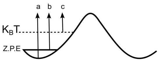
Figure 2.
The effect of zero-point energy and temperature on the MAE of an arbitrary barrier. The energy of the electronic state of the system is increased such that the bottom of the potential well is no longer accessible, leading to a decrease in the effective barrier, which change the MAE from being represented by arrow a to arrow b. Increasing the temperature will lead to arrow c.
2.2. Quasiparticle Picture of Magnetic Anisotropy
The standard picture of magnetic anisotropy — that of an external field "pushing" spins from one configuration to another — is somewhat troubling when one considers the linear magnetic field alignment in experimental measures of anisotropy [7], as this cannot produce an angular rotation of spins. This is because there is never a component of the applied field perpendicular to the spins. It may then be preferable to consider a quasiparticle picture of the anisotropy, in an analogous way to considering soft phonons to model phase transitions [22]. This does not change the underlying physics but simply uses different language to describe it, which makes the physical processes more apparent.
In this picture, any arbitrary magnetic structure can be written as a sum of the ground-state magnetic structure and a collection of symmetry-appropriate magnons. For the rotation of the ground state to its symmetric partner (exchanging up and down labels), this corresponds to a long-wavelength acoustic magnon.
This gives rise to the current strategy for evaluating MAE; calculate (or measure) the creation energy of this particular excitation to the spin structure with a static structure. However, if the minimum energy (transition) pathway (MEP) follows a route that requires a structural relaxation, then a quasiparticle responsible for this (a phonon) must be generated simultaneously to the magnon. This scenario is shown in Figure 3.
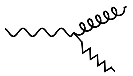
Figure 3.
A schematic Feynmann diagram for the calculation of MAE. An incoming photon enables the creation of a magnon (and a phonon if magnetostuctural coupling provides the MEP), thereby driving the magnetic transition.
In terms of quasiparticles, the experimentally measured MAE is the energy loss due to the generation of either the magnon directly or the magnon–phonon pair (for the bound pair where they act as a single quasiparticle rather than as two coexisting quasiparticles, we use the term “magnetophonon”). Simulating the MAE then requires one to evaluate the creation energy of all of these pathways. The authors note that further expansions in terms of additional interactions are possible, such as multiple phonon and multiple magnon excitations; however the contribution of these higher order terms to the expansion are smaller, and therefore are neglected here.
One final subtlety of note is that magnons and phonons are Majorana particles — that is, they are their own antiparticles [23] — and accordingly, one can read the Feynman diagram in Figure 3 in multiple ways. The most obvious are the two solutions that come from considering the phonon as an emitted (see Equation (1)) or absorbed particle (Equation (3)). Additionally, one may consider the case where no phonon interactions are involved (Equation (2)). We have
This makes the experimentally measured MAE an expectation value of the multiple pathways with appropriate weighting with the final experimentally measured barrier given as
where are the Arrhenius factors for each route and may be expressed as
where is the Arrhenius prefactor for route i. This gives an explicit temperature dependence for the MAE and means that when , the lowest energy route will dominate the kinetics. In order to evaluate the MAE at any arbitrary temperature (that is, below the critical temperature for the relevant magnetic phase), all that is required is to evaluate the energy of the individual routes and the Arrhenius prefactor. This prefactor may be thought of as the rate at which a system may attempt to overcome the transition barrier.
We also note that although a continuum of pathways for the spin flip exists, because the energy landscape is continuous, we only consider the routes that are lowest in energy for any given conditions. An experiment will average over all possible pathways, with those that are lower in energy dominating due to the exponential factor within Equation (5) (the Arrhenius equation).
2.3. Attempt Frequency
It is well known that a further important property when interpreting experimental data relating to the anisotropy is the attempt frequency [24,25]. This is typically stated to be a constant characteristic frequency for spin-flipping events (and therefore corresponds to the Arrhenius prefactor). It is notable that the attempt frequency for antiferromagnetic materials (10 Hz) [25] is three orders of magnitude higher than for ferromagnetic materials (10 Hz) [26] and also that these are of the same order of magnitude as the reciprocal phonon–phonon lifetimes for acoustic and optical phonons, respectively [27].
A possible explanation for this is outlined in schematic form in Figure 4. In this scenario, the specific magnon mode commensurate with a spin-transition and its commensurate phonon (which must have the appropriate symmetry to couple strongly with this magnon mode) are abstracted from two general baths of magnons and phonons respectively, and specific transition rates between all four (and internal conversions for the bath) are considered. In the strong magnon–phonon coupling limit (), these two modes form a single magnetophonon and may be considered as a single quasiparticle, which may be scattered by either magnons or phonons. By considering rate equations and requiring the system to be in a dynamic equilibrium, we may determine rates of conversion between and the populations of all levels.
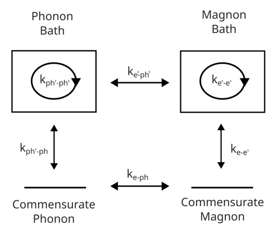
Figure 4.
Schematic of the possible interactions between the magnon associated with the selected spin transition, its commensurate phonon, and the baths of available phonon and magnon states.
First, we define an attempt as the creation of a magnon-like quasiparticle (either a magnon or magnetophonon) that is commensurate with changing the state of the electronic system to the barrier in spin-space between up and down configurations. Because these quasiparticles are bosonic, there is no limit to the amount of population of a single mode, so accordingly there are no density-of-states considerations in the transition rates, only requirements for conservation of energy and momentum which then yield selection rules.
By the principle of detailed balance, for a system in equilibrium (or near to equilibrium in the adiabatic limit) the rates of creation and annihilation of the magnon/magnetophonon mode must be equal (otherwise the population of the mode will change and the system is not in equilibrium). This suggests that the attempt frequency is the lifetime of the magnon/magnetophonon, which for the case of the magnetophonon may be calculated from the magnon and phonon scattering rates by using Matthiessen’s rule,
where is the lifetime of the respective quasiparticle. The lifetime of the magnon seems unlikely to change significantly for different spin structures, as the magnon will remain acoustic (an optical mode corresponds to an FM-AFM transition). The magnon and phonon lifetimes will be dominated by scattering into their respective baths, and therefore the lifetime of the magnetophonon will be lower than the shorter of the phonon and magnon lifetimes. This magnetophonon picture (rather than the bare-magnon) explains the finding that AFM materials have a higher attempt frequency; they couple to optical phonons with a shorter lifetime, thereby increasing the attempt frequency, which may be represented as .
2.3.1. Symmetry Considerations
There are symmetry considerations with regard to the selection of which magnon and phonon modes couple together to form the magnetophonon associated with the MAE. For the magnon modes, the magnon drives the reorientation of the spins with respect to the crystal axes, and the lowest energy magnon mode is an acoustic mode in the long wavelength limit (). This mode rotates all spins across all space uniformly.
Any phonon mode coupled to this must affect all of space in the same way as the magnon (), but whether it is an acoustic or an optical mode depends on whether the system is ferromagnetic (in which case it will be acoustic) or antiferromagnetic (in which case the opposite responses of the different sublattices will lead to an optical phonon).
One result of this is that applying a magnetic field to a ferromagnetic system will also generate an acoustic phonon, leading to a volume change (magnetostriction). Conversely, applying a magnetic field to an antiferromagnetic system will generate an optical phonon (which conserves the volume) and so there will not be any magnetostriction. This behaviour is in agreement with previous studies on other magnetic systems [28].
It is also worth noting that the energy of a acoustic phonon is vanishingly small, which suggests that the overall effect on the MAE of the magnon–phonon coupling will also be very small. However, this is not true for an optical phonon, and therefore the effect should be significantly larger in AFM materials than in FM materials.
2.3.2. Conservation of Energy
The energy for the creation of the magnon (or magnetophonon) that drives the transition cannot come from the applied magnetic field. The total energy of a 1 T magnetic field, as typically used in experiments, in a volume of free space equal to the size of a crystallographic unit cell is ∼0.3 meV — and the energy per photon in this region will be even smaller. Hence, the external field only serves to couple different electronic states together, thereby enabling the stimulated rather than spontaneous generation of our commensurate magnon (magnetophonon). The energy to drive the transition, therefore, comes not from the external applied field but rather from internal sources of energy (and therefore, indirectly, the environment), namely the magnon heat bath and the phonon heat bath. Hence, this is a case of photon-assisted magnon–phonon conversion (in contrast to [29], which use phonons under illumination to generate magnons). The applied field enables the transition between different electronic states of the system to occur, whereas the energy comes from internal conversion due to scattering from phonon and magnon modes that have been thermally populated.
Considering that these two heat baths are connected [30,31] and the material is at a constant temperature (in thermal equilibrium), the magnon and phonon bath may be expected to have an equal distribution of energy, under the principle of equipartition. This suggests that there are two types of routes leading to the creation of the acoustic magnon that corresponds to the MAE. The first of these routes is the “standard” route, which is purely magnonic, and involves no structural relaxations (except as a subsequent potential decay path for the commensurate magnon). The second type of route is the phononic routes identified in Section 2.2 ( or ). These routes involve scattering within the phonon bath to populate a mode that obeys the same symmetries as the commensurate magnon (or in the magnetophonon case, is the same quasiparticle).
These two phononic routes differ in that the route treats the magnon and phonon as a single quasiparticle, whereas the route treats them as two independent quasiparticles. Which of these regimes dominates (and therefore controls the “fastest switching pathway” MAE for an AFM material) depends on the coupling strength between the magnon associated with the MAE and its associated phonon [31]. For magnons and phonons, the low momentum leads to a large uncertainty in the position of both quasiparticles and therefore, within the relaxation time approximation, the coupling should be extremely large (), leading to being the dominant route. In this strong coupling limit (), it does not make sense to consider magnons and phonons separately, but rather as a single magnetophonon [32].
2.4. Recap
- The MAE is the minimum energy barrier to transition between two magnetic states which correspond to easy axis alignment.
- This corresponds to the creation of a magnon mode, which may or may not be simultaneously coupled to a phonon mode (a magnetophonon).
- For FM materials, this phonon mode is a long-wavelength acoustic mode and consequently should only give a small correction to the MAE, but will generate magnetostriction.
- For AFM materials, this phonon mode is a long-wavelength optical mode, and consequently will provide a more significant change to the MAE due to the higher energy of the optical mode, and no magnetostriction.
- When the magnon–phonon coupling between these modes is strong, the MAE is represented by a magnetophonon that has a different energy to either the magnon or phonon when they are considered separately.
- Coupling to an optical rather than an acoustic mode has a three-orders of magnitude effect on the attempt frequency due to the difference in phonon lifetimes, leading to faster switching speeds for AFM-based devices.
3. Methodology
3.1. Density Functional Theory Parameters
The plane-wave DFT [33,34] code CASTEP [35] was used to simulate the MAE by evaluating the total energy of a conventional unit cell as the orientation of the spin moments on the non-Pt (Fe or Mn) ions—where the majority of the spin in the system is located—were rotated by applying spin constraints. Fully relativistic pseudopotentials from the CASTEP SOC19 pseudopotential library were used with vector spin-modelling and spin-orbit coupling in order to capture this effect. Because both FePt and PtMn are metals, the Perdew–Zunger formulation [36] of the local density approximation (LDA) was used and may be expected to perform acceptably well.
Although more sophisticated treatments of exchange-correlation are available for the collinear limit, many do not yet have explicit noncollinear reformulations [37]. However, the methodological improvements suggested in this paper are independent of the choice of exchange-correlation functional, and therefore it is sufficient to demonstrate these benefits for the LDA, despite the fact that other choices might improve other aspects of the physical model.
Numerical convergence of the plane wave basis set was performed to ensure total energy convergence of 0.01 meV/atom (2100 eV plane wave cutoff), and the same tolerance was used to converge the k-space sampling (a Monkhorst-Pack grid [38] for PtMn and for FePt).
Applied Constraints
In order to sample the potential energy surface away from the global minimum, spin constraints were applied to ensure that the desired spin configuration was achieved through a method of Lagrangian minimization [39]. To this end, a constraint that vanishes at the desired spin-configuration but was positive (destabilising) elsewhere was applied. This ensured that the correct value of the potential energy landscape was sampled for the constraint configuration, but also that this was an artificial minimum in the energy landscape such that the minimisation of the total energy could identify this as the appropriate ground state of the system. This technique is conceptually similar to metadynamics [40], and ensures that both the true potential energy surface as well as non-ground-state spin configurations can be sampled.
3.2. Geometry Optimisation Parameters
The structures were relaxed by using BFGS minimisation until stresses were lower than GPa and forces were less than eV/Å, and a finite basis correction was used to ensure constant basis quality.
During the geometry optimisation, spatial symmetry operations were not enforced. This is because the magnetic ordering lowers the symmetry of the crystal structure (always for the AFM, and for the FM whenever the spins are not aligned along the c-axis), and it was necessary to remove any potential "false symmetries" that may be present which could lead to force cancellation by symmetry.
Additionally, a collinear LDA+U relaxation of the structures was performed, with an effective U correction of 4.5 eV applied to the Mn 3d orbitals and 3.5 eV to the Fe 3d orbitals. The MAE for this LDA+U relaxed structure was then evaluated by using the previous method with no Hubbard correction applied.
4. Results and Discussion
4.1. Materials
FePt is an exemplar high-anisotropy ferromagnetic material which has an L0 structure (see Figure 5a). PtMn is the AFM equivalent of FePt, with the only differences emerging from substituting Fe for Mn (see Figure 5b). This substitution yields significant differences to the magnetic structure (which changes from collinear FM to collinear C-type AFM) but not the crystal structure or the magnitude of the spin-orbit coupling introduced by the “heavy metal ion” Pt, which is constant between both.
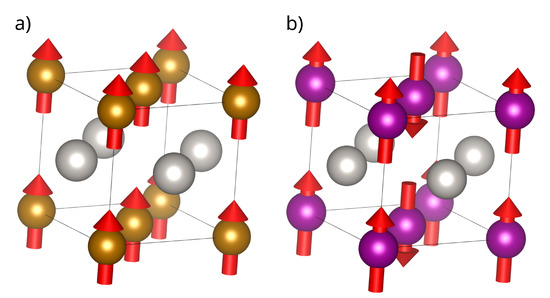
Figure 5.
(a) The ground-state magnetic and geometric structure of FePt. (b) The ground-state magnetic and geometric structure of PtMn. Brown atoms are Fe, purple atoms are Mn and silver are Pt. Note that the major difference between these structures is in the magnetic coupling between the Fe atoms and the Mn atoms.
4.2. Magnetic-Only Transition State
In order to perform the magnetic-only (LST-like) transition search—corresponding to the standard method with clamped ions—a series of “sweeps” were performed by varying the spin orientation from (+) to (). These sweeps varied by their orientation (angle to ) in order to ensure a good coverage of the magnetic phase space. Due to the symmetry of the crystals, the variation is periodic with a period of 90 degrees. It is also a minor variation compared with the variation in , and accordingly in the interest of clarity only the sweeps at 0 and 45 degrees have been reported.
4.2.1. FePt
For FePt, the sweeps are shown in Figure 6. We observe the expected behaviour (including higher order terms, as expected from an ab initio model). Additionally, the dependence is observed to be very weak, although with a very slightly softer axis, which is the minimum energy pathway through magnetic space only for the LDA unit cell. Nevertheless, this -variation is so weak that FePt may be said to exhibit uniaxial anisotropy with a hard plane.
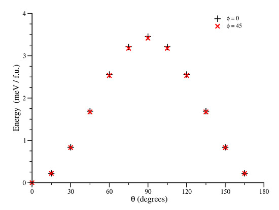
Figure 6.
Variation of total energy (in meV / f.u.) with angle from the easy axis, , for two values of the azimuthal angle, and for FePt. is expected to be the dominant term under the uniaxial approximation.
The MAE from these results (3.45 meV/f.u., see Figure 6) were found to agree with certain literature results [41] but to be in relatively poorer agreement with others [8]. This was driven by the choice of lattice parameters — in this work we have used the relaxed LDA geometry with no Hubbard-U correction, but other works [8] have used values nearer the bulk experimental lattice parameters (the relaxed LSDA+U geometry). Using the same lattice parameters as these other works (, ) yielded the same values as they reported (2.68 meV/f.u. using our method compared with 2.68 meV/f.u. for the calculation on the same cell [8]). Thus, the choice of geometry clearly has an effect on the evaluated MAE; the overbinding of LDA leads to shorter “bonds” and therefore increased effective spin-orbit interactions for the Fe orbitals (which have hybridised with Pt orbitals), and also a higher crystal field splitting of the orbitals—thereby increasing the calculated anisotropy. Nevertheless, in order to avoid mixing different approximations to the exchange-correlation functional, we have chosen to evaluate all of our MAEs at the bulk LDA lattice parameters with no Hubbard-U corrections.
In addition, we calculated the variation of the MAE with applied biaxial strain (keeping the lattice vector fixed and measuring the value of the MAE at several values) as shown in Figure 7. This clearly demonstrates that the MAE is dependent upon the strain of the system. Although not perfectly linear, there is a clear linear trend, which may be indicative of decreasing effective spin-orbit coupling for electrons predominantly centred on Fe atoms as the overlap between Fe and Pt d-orbitals decreases.
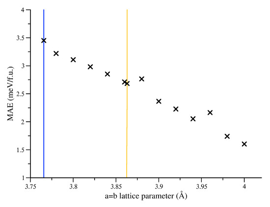
Figure 7.
Change of energy difference between - and -aligned spin structures with strain for FePt. This figure includes both the LDA (blue line) and LDA+U (yellow line) structures at their exact in-plane lattice parameter.
4.2.2. PtMn
The angular sweeps for PtMn are shown in Figure 8. The predicted anisotropy per formula unit is lower than for FePt (as expected), and shows the same behaviour with strongly uniaxial behaviour. In this case, the orientation provides a fractionally lower energy pathway; however, this is not resolvable in Figure 8. We also note that the energy per formula unit is not the same as the energy for the unit cell, although a conventional unit cell is required to model the magnetic structure the formula unit is explicitly 1 Pt and 1 Mn.
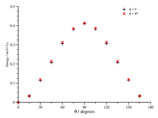
Figure 8.
Variation of total energy (in meV) with angle from the easy axis, , for two values of the azimuthal angle, and .
In addition to the full angular sweep shown in Figure 8, the MAE was evaluated for various systems with biaxial strain (along and axes) applied in order to mimic the effects of growth seed layer choice upon the MAE. These results are shown in Figure 9. The total range of strains evaluated, of the order of , is large, but not unreasonable in the thin film limit typically used to grow samples. As for FePt, the MAE was evaluated for all systems (including the LDA + U geometry) without applied Hubbard-U. This does not, however, capture the direct effects of the applied-U to the MAE beyond the effects induced by the change in lattice parameters.
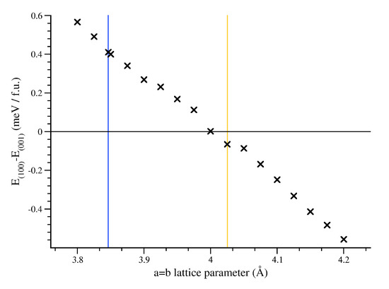
Figure 9.
Change of energy difference between - and -aligned spin structures with strain. Note that the MAE is the absolute value of this number, and the sign change indicates a strain-induced alteration of the easy and hard magnetic axes. The blue line represents the LDA lattice parameter, and the yellow line indicates the LDA + U lattice parameter.
The change of MAE with strain shown in Figure 9 indicates a strong dependence of the MAE on the underlying geometry. These are large changes—and so the underlying assumptions of the phonon-based model of small amplitude oscillations are not applicable—and accordingly a large change in anisotropy is seen. In addition to the obvious ability this gives to engineer thin-film anisotropy based upon a careful choice of seed layer, it should also be able to create electrical control of the MAE by coupling a PtMn layer with a piezoelectric layer.
We also note that these results are in qualitative agreement with other recent theoretical efforts which considered varying both the and lattice parameters [42]. On the other hand, it seems likely that this change is driven by the changing crystal field splitting at the Mn sites driven by the change of interatomic distances rather than the ratio per se.
4.3. Magnetostructural Transition State
Following the identification of the peak of the magnetic anisotropy (the hard axis), the structure was relaxed in order to perform the QST-like search throughout the orthogonal structure space (as opposed to the spin space). For a maximum, such as the magnetic-only transition state, there are formally no forces, because it is a stationary point. Accordingly, several small initial perturbations were applied to this structure before the relaxation was performed. This is to ensure that the symmetry of the system is broken to enable the unit cell to relax (as the forces are zero at a maximum).
4.3.1. FePt
The relaxed geometry of L0 FePt was found for both the easy and hard magnetic configurations through geometry optimisation of the lattice parameters with the magnetic configuration constrained to the easy and hard axes respectively. The ions remained at high symmetry points. The lattice parameters given by these relaxation are given in Table 1.

Table 1.
Lattice parameters for relaxed PtMn dependant upon the different spin configurations. LDA + U and experimental lattice parameters are also provided for comparison.
These relaxations show a small (0.02 ) increase in total cell volume and a breaking of the symmetry of the unit cell for the hard magnetic configuration. This is in agreement with the previous arguments about magnetostriction in FM materials.
Following relaxation, the total energy of the system for all combinations of these spin and geometry configurations were evaluated (results shown in Table 2).
Table 2.
Relative energies (in meV/formula unit) for the various configurations of spin and geometry in FePt. The easy geometry is the ground-state geometry of the system, and the hard geometry is the relaxed geometry of the system under the constraint that the system is aligned along the magnetic hard axis.
It is clear that the structural relaxation is a small effect (∼0.5% )—in line with the ∼0.1% lattice parameter change. However, this is per formula unit; for a macroscopic layer of FePt, this effect is multiplied up until these apparently small energy barriers become significant—with even the small difference between easy and hard geometries for the easy spin configuration becoming a barrier larger than when 200 conventional unit cells are present.
Finally, it is worth noting that in addition to the thermodynamic arguments here, there are also dynamical considerations. As discussed in Section 2.2 and Section 2.3, there are three possible routes from the magnetic easy to the magnetic hard axis: , corresponding to a fixed easy axis geometry; corresponding to a direct change from the easy geometry to the hard geometry; and corresponding to a fixed hard axis geometry. The attempt frequency for these different routes varies significantly and therefore, in a short time period such as in a data read or write process, the route with the highest attempt rate that is thermally accessible is likely to dominate. In a data-storage scenario, however, the long time period means that the lowest energy route is likely to be favoured.
For FePt these considerations are small. The difference in the barrier between and —the routes with the largest difference in energy—is less than 1%, making the choice of protocol a smaller effect than other errors associated with the choice of functional or geometry used. This is in accord with the very low energy of the acoustic phonon mode. For AFM materials, however, the relatively large energy of the optical phonon mode must be considered.
4.3.2. PtMn
The same procedure was carried out for antiferromagnetic L1 PtMn, and the structural changes are shown in Table 3. As anticipated, the observed magnetostriction was small (<2 mÅ) and may be attributed to remnant FM couplings between the component of the spins, which are canted by the Dzyaloshinskii–Moriya interaction (DMI). The magnitude of DMI is expected to be small because it leads to the presence of a spin-spiral ground state when it is strong [44]. The largest effect on the structure is a very small movement of the Pt ion in , which corresponds to the 22 meV transverse optical (TO) mode of the system. At first it may seem surprising that the Pt ions should move in response to the reorientation of the spins at the Mn sites, but this may be explained by considering that the movement of the Pt ions affects both the strength and symmetry of the crystal field experienced at the Mn sites. This perturbation changes the energy of individual bands, thereby leading to a reduction in energy of the system when the spins are aligned along the hard axis.
Table 3.
Lattice parameters and atomic positions for relaxed PtMn dependant upon the different spin configurations.
The key change in the structure is the perturbation of the Pt atoms (unlike the FePt case in which they remained stationary at the high symmetry positions). This change, corresponding to a TO phonon mode of 22 meV, is in agreement with previously reported values of 18 meV (4.3 THz) [42]. DFT LDA calculations (as used here) overbind and hence give higher phonon frequencies, whereas PBE (as used in ref [42]) underbinds and hence gives slightly lower phonon frequencies.
With PtMn, unlike FePt, the energy of the system with spin aligned along the hard axis does not significantly change when the geometry is relaxed (in agreement with the fact that antiferromagnetic systems do not respond strongly to applied fields). However, when the hard-axis relaxed geometry is measured in the easy-axis configuration, a significant increase in the energy is observed, as shown in Table 4.
Table 4.
Relative energies (in meV/f.u.) for the various configurations of spin and geometry in PtMn. The easy geometry is the ground-state geometry of the system, and the hard geometry is the geometry of the system having been relaxed under the constraint that the system is aligned along the magnetic hard axis.
Now, the displacement that leads to this increase in energy is very small (≈2.9 mÅ). This is actually smaller than the zero-point amplitude of the phonon mode associated with (≈18.7 mÅ). The fact that this displacement is smaller than the zero-point motion—which is an effective permanent population of the relevant phonon mode—means that this lower energy route, , is always achievable. Also unlike FePt, the effect of this small displacement is to significantly reduce the MAE from 0.41 meV/f.u. to 0.32 meV/f.u., which is an ∼20% reduction in the size of the theoretical barrier.
Although the absolute magnitude of these effects will vary with the level of theory used in DFT for the system under investigation—for example, the use of a GGA or Hubbard-U correction might be expected to remove the overbinding of LDA and make the model of the system more accurate—the effect of the magnetostructural coupling on the MAE will remain. Although it is a negligible effect in ferromagnetic systems, this work shows that it is a significant effect for antiferromagnetic systems. Hence, it should be included in all calculations of MAE in AFMs, even with higher levels of theory, if the MAE is to be accurately modelled and not systematically overestimated.
5. Conclusions
The MAE was evaluated for ferromagnetic FePt and antiferromagnetic PtMn and found to be 3.45 meV/f.u. and 0.41 meV/f.u., respectively, for the LDA approximation in the static-ion limit. The choice of lattice parameters (for example LDA vs LDA+U geometries) was found to provide a significant change in the calculated MAE, up to an exchange of the easy and hard axes of the system. Relaxing the systems to find the magnetostructural rather than just the magnetic transition states yielded a ∼1% reduction in the barrier height of FePt (to 3.44 meV/f.u.), and a ∼20% reduction for PtMn (to 0.32 meV/f.u.) when the lowest energy pathway was considered. This difference is attributed to the difference in coupling between the magnon responsible for the transition and either an acoustic or optical phonon (for FePt and PtMn respectively). This shows the importance of considering magnetostructural effects when evaluating the MAE of systems in which the magnetic structure cannot be adequately expressed in the same primitive unit cell as the geometric structure, such as an antiferromagnet.
Author Contributions
Conceptualization and investigation, R.A.L.; writing—original draft preparation, R.A.L.; writing—review and editing, S.J.D.; visualization, R.A.L. and S.J.D.; supervision, resources, project administration and funding acquisition, M.I.J.P. All authors have read and agreed to the published version of the manuscript.
Funding
Computational support was provided by the UK national high performance computing service, ARCHER2, for which access was obtained via the UKCP consortium and funded by EPSRC grant ref EP/P022561/1. The authors also acknowledge EPSRC grant EP/V047779/1 for financial support.
Institutional Review Board Statement
Not applicable.
Informed Consent Statement
Not applicable.
Data Availability Statement
The data presented in this study are openly available in the York Research Database at doi:10.15124/b1ec96de-4796-45a6-89f9-dc0c34d0f431.
Acknowledgments
The authors would like to thank Jerome Jackson, Kevin O’Grady and Gonzalo Vallejo Fernandez for their kind comments and valuable conversations in preparing this work.
Conflicts of Interest
The authors declare no conflict of interest.
References
- Mattioli, M. The Apollo Guidance Computer. IEEE Micro 2021, 41, 179–182. [Google Scholar] [CrossRef]
- Nordrum, A. The fight for the future of the disk drive. IEEE Spectr. 2019, 56, 44–47. [Google Scholar] [CrossRef]
- Wang, K.L.; Alzate, J.G.; Amiri, P.K. Low-power non-volatile spintronic memory: STT-RAM and beyond. J. Phys. D: Appl. Phys. 2013, 46, 074003. [Google Scholar] [CrossRef]
- Kosub, T.; Kopte, M.; Hühne, R.; Appel, P.; Shields, B.; Maletinsky, P.; Hübner, R.; Liedke, M.O.; Fassbender, J.; Schmidt, O.G.; et al. Purely antiferromagnetic magnetoelectric random access memory. Nat. Commun. 2017, 8, 13985. [Google Scholar] [CrossRef]
- Charap, S.; Lu, P.L.; He, Y. Thermal stability of recorded information at high densities. IEEE Trans. Magn. 1997, 33, 978–983. [Google Scholar] [CrossRef]
- Martins, A.; Trippe, S.; Santos, A.; Pelegrini, F. Spin-wave resonance and magnetic anisotropy in FePt thin films. J. Magn. Magn. Mater. 2007, 308, 120–125. [Google Scholar] [CrossRef]
- O’Grady, K.; Fernandez-Outon, L.; Vallejo-Fernandez, G. A new paradigm for exchange bias in polycrystalline thin films. J. Magn. Magn. Mater. 2010, 322, 883–899. [Google Scholar] [CrossRef]
- Shick, A.B.; Mryasov, O.N. Coulomb correlations and magnetic anisotropy in ordered L10 CoPt and FePt alloys. Phys. Rev. B 2003, 67, 172407. [Google Scholar] [CrossRef]
- Khan, S.A.; Blaha, P.; Ebert, H.; Minár, J.; Šipr, O. Magnetocrystalline anisotropy of FePt: A detailed view. Phys. Rev. B 2016, 94, 144436. [Google Scholar] [CrossRef]
- Nauman, M.; Kiem, D.H.; Lee, S.; Son, S.; Park, J.G.; Kang, W.; Han, M.J.; Jo, Y. Complete mapping of magnetic anisotropy for prototype Ising van der Waals FePS3. 2D Mater. 2021, 8, 035011. [Google Scholar] [CrossRef]
- Higgins, E.J.; Hasnip, P.J.; Probert, M.I. Simultaneous Prediction of the Magnetic and Crystal Structure of Materials Using a Genetic Algorithm. Crystals 2019, 9, 439. [Google Scholar] [CrossRef]
- Zhu, B.; Lu, Z.; Pickard, C.J.; Scanlon, D.O. Accelerating cathode material discovery through ab initio random structure searching. APL Mater. 2021, 9, 121111. [Google Scholar] [CrossRef]
- Burkert, T.; Eriksson, O.; Simak, S.I.; Ruban, A.V.; Sanyal, B.; Nordström, L.; Wills, J.M. Magnetic anisotropy of L10 FePt and Fe1-xMnxPt. Phys. Rev. B 2005, 71, 134411. [Google Scholar] [CrossRef]
- Shick, A.B.; Máca, F.; Lichtenstein, A.I. Magnetic anisotropy of single 3d spins on a CuN surface. Phys. Rev. B 2009, 79, 172409. [Google Scholar] [CrossRef]
- Jónsson, H.; Mills, G.; Jacobsen, K.W. Nudged elastic band method for finding minimum energy paths of transitions. In Classical and Quantum Dynamics in Condensed Phase Simulations: Proceedings of the International School of Physics, Lerici, Villa Marigola, 7–18 July 1997; Berne, B., Ciccoti, G., Coker, D.F., Eds.; World Scientific: Singapore, 1998. [Google Scholar] [CrossRef]
- Henkelman, G.; Uberuaga, B.P.; Jónsson, H. A climbing image nudged elastic band method for finding saddle points and minimum energy paths. J. Chem. Phys. 2000, 113, 9901–9904. [Google Scholar] [CrossRef]
- Halgren, T.A.; Lipscomb, W.N. The synchronous-transit method for determining reaction pathways and locating molecular transition states. Chem. Phys. Lett. 1977, 49, 225–232. [Google Scholar] [CrossRef]
- Peterson, A.A. Acceleration of saddle-point searches with machine learning. J. Chem. Phys. 2016, 145, 074106. [Google Scholar] [CrossRef] [PubMed]
- Hammond, G.S. A Correlation of Reaction Rates. J. Am. Chem. Soc. 1955, 77, 334–338. [Google Scholar] [CrossRef]
- Zhu, Y.A.; Dai, Y.C.; Chen, D.; Yuan, W.K. First-principles calculations of CH4 dissociation on Ni(100) surface along different reaction pathways. J. Mol. Catal. A: Chem. 2007, 264, 299–308. [Google Scholar] [CrossRef]
- Lechner, B.A.J.; Hedgeland, H.; Ellis, J.; Allison, W.; Sacchi, M.; Jenkins, S.J.; Hinch, B.J. Quantum Influences in the Diffusive Motion of Pyrrole on Cu(111). Angew. Chem. Int. Ed. 2013, 52, 5085–5088. [Google Scholar] [CrossRef]
- Rudin, S.P. Generalization of soft phonon modes. Phys. Rev. B 2018, 97, 134114. [Google Scholar] [CrossRef]
- Wilczek, F. Majorana returns. Nat. Phys. 2009, 5, 614–618. [Google Scholar] [CrossRef]
- Vallejo-Fernandez, G.; Aley, N.P.; Chapman, J.N.; O’Grady, K. Measurement of the attempt frequency in antiferromagnets. Appl. Phys. Lett. 2010, 97, 222505. [Google Scholar] [CrossRef]
- Roca, A.G.; Vallejo-Fernández, G.; O’Grady, K. An Analysis of Minor Hysteresis Loops of Nanoparticles for Hyperthermia. IEEE Trans. Magn. 2011, 47, 2878–2881. [Google Scholar] [CrossRef]
- Sharma, S.; Shallcross, S.; Elliott, P.; Dewhurst, J.K. Making a case for femto-phono-magnetism with FePt. Sci. Adv. 2022, 8. [Google Scholar] [CrossRef] [PubMed]
- Maldonado, P.; Carva, K.; Flammer, M.; Oppeneer, P.M. Theory of out-of-equilibrium ultrafast relaxation dynamics in metals. Phys. Rev. B 2017, 96, 174439. [Google Scholar] [CrossRef]
- Liu, S.; del Águila, A.G.; Bhowmick, D.; Gan, C.K.; Do, T.T.H.; Prosnikov, M.; Sedmidubský, D.; Sofer, Z.; Christianen, P.C.; Sengupta, P.; et al. Direct Observation of Magnon-Phonon Strong Coupling in Two-Dimensional Antiferromagnet at High Magnetic Fields. Phys. Rev. Lett. 2021, 127, 097401. [Google Scholar] [CrossRef]
- fan Qi, S.; Jing, J. Magnon-assisted photon-phonon conversion in the presence of structured environments. Phys. Rev. A 2021, 103, 043704. [Google Scholar] [CrossRef]
- Aguilar, R.V.; Sushkov, A.B.; Zhang, C.L.; Choi, Y.J.; Cheong, S.W.; Drew, H.D. Colossal magnon-phonon coupling in multiferroic Eu0.75Y0.25MnO3. Phys. Rev. B 2007, 76, 060404. [Google Scholar] [CrossRef]
- Man, H.; Shi, Z.; Xu, G.; Xu, Y.; Chen, X.; Sullivan, S.; Zhou, J.; Xia, K.; Shi, J.; Dai, P. Direct observation of magnon-phonon coupling in yttrium iron garnet. Phys. Rev. B 2017, 96, 100406. [Google Scholar] [CrossRef]
- Shen, P.; Kim, S.K. Magnetic field control of topological magnon-polaron bands in two-dimensional ferromagnets. Phys. Rev. B 2020, 101, 125111. [Google Scholar] [CrossRef]
- Hohenberg, P.; Kohn, W. Inhomogeneous electron gas. Phys. Rev. 1964, 136, B864–B871. [Google Scholar] [CrossRef]
- Kohn, W.; Sham, L.J. Self-consistent equations including exchange and correlation effects. Phys. Rev. 1965, 140, A1133–A1138. [Google Scholar] [CrossRef]
- Clark, S.J.; Segall, M.D.; Pickard, C.J.; Hasnip, P.J.; Probert, M.J.; Refson, K.; Payne, M. First principles methods using CASTEP. Z. Kristall. 2005, 220, 567–570. [Google Scholar] [CrossRef]
- Perdew, J.P.; Zunger, A. Self-interaction correction to density-functional approximations for many-electron systems. Phys. Rev. B 1981, 23, 5048–5079. [Google Scholar] [CrossRef]
- Scalmani, G.; Frisch, M.J. A New Approach to Noncollinear Spin Density Functional Theory beyond the Local Density Approximation. J. Chem. Theory Comput. 2012, 8, 2193–2196. [Google Scholar] [CrossRef]
- Monkhorst, H.J.; Pack, J.D. Special points for Brillouin-zone integrations. Phys. Rev. B 1976, 13, 5188–5192. [Google Scholar] [CrossRef]
- Cuadrado, R.; Pruneda, M.; García, A.; Ordejón, P. Implementation of non-collinear spin-constrained DFT calculations in SIESTA with a fully relativistic Hamiltonian. J. Phys. Mater. 2018, 1, 015010. [Google Scholar] [CrossRef]
- Laio, A.; Parrinello, M. Escaping free-energy minima. Proc. Natl. Acad. Sci. USA 2002, 99, 12562–12566. [Google Scholar] [CrossRef]
- Barreteau, C.; Spanjaard, D. Magnetic and electronic properties of bulk and clusters of FePt L10. J. Phys. Condens. Matter 2012, 24, 406004. [Google Scholar] [CrossRef]
- Aissat, D.; Baadji, N.; Mazouz, H.; Boussendel, A. Connection between lattice parameters and magnetocrystalline anisotropy in the case of L10 ordered antiferromagnetic MnPt. J. Magn. Magn. Mater. 2022, 563, 170013. [Google Scholar] [CrossRef]
- Klemmer, T.J.; Shukla, N.; Liu, C.; Wu, X.W.; Svedberg, E.B.; Mryasov, O.; Chantrell, R.W.; Weller, D.; Tanase, M.; Laughlin, D.E. Structural studies of L10 FePt nanoparticles. Appl. Phys. Lett. 2002, 81, 2220–2222. [Google Scholar] [CrossRef]
- Hervé, M.; Dupé, B.; Lopes, R.; Böttcher, M.; Martins, M.D.; Balashov, T.; Gerhard, L.; Sinova, J.; Wulfhekel, W. Stabilizing spin spirals and isolated skyrmions at low magnetic field exploiting vanishing magnetic anisotropy. Nat. Commun. 2018, 9, 1015. [Google Scholar] [CrossRef]
- Mao, S.; Gao, Z. Characterization of magnetic and thermal stability of PtMn spin valves. IEEE Trans. Magn. 2000, 36, 2860–2862. [Google Scholar] [CrossRef]
Disclaimer/Publisher’s Note: The statements, opinions and data contained in all publications are solely those of the individual author(s) and contributor(s) and not of MDPI and/or the editor(s). MDPI and/or the editor(s) disclaim responsibility for any injury to people or property resulting from any ideas, methods, instructions or products referred to in the content. |
© 2023 by the authors. Licensee MDPI, Basel, Switzerland. This article is an open access article distributed under the terms and conditions of the Creative Commons Attribution (CC BY) license (https://creativecommons.org/licenses/by/4.0/).