Estimation of Radiation Damping Rates Using ¹³³Cs, ⁷Li and ³¹P Solution NMR Spectroscopy and a Theoretical NMR RASER Model

Abstract

Radio amplification using stimulated emission of radiation (RASER) effects in the NMR can increase NMR signals over time due to a feedback loop between the sample magnetization and the probe coil coupled with radiation damping (RD). Previously, RD rates had been directly observed only for the ¹H, ³He, ¹⁷O and ¹²⁹Xe nuclei. We report that experimental direct measurements of an NMR RASER to determine RD time constants for the three heteronuclei (¹³³Cs (I = 7/2), ⁷Li (I = 3/2) and ³¹P (I = 1/2)) in a highly concentrated solution from the NMR RASER emissions using a conventional NMR probe. Under conditions where the RD rate exceeds the transverse relaxation rate (i.e., the NMR RASER condition is fulfilled), we recorded both the transverse NMR RASER response to imperfect inversion and the recovery of longitudinal magnetization. The data were directly evaluated based on the well-known Bloom model as estimated RD rate constants of 8.0, 1.8 and 25 Hz for ¹³³Cs, ⁷Li and ³¹P, respectively. The proposed method can be applied to observe RD rate constants for the other nuclei as well.

1. Introduction

NMR radio frequency amplification using stimulated emission of radiation (RASER) is a phenomenon that leads to an increase in NMR signals with time through a feedback loop between the probe coil and longitudinal magnetization, when starting from (partially) inverted magnetization. NMR RASERs have only been observed in the ¹H [1,2,3,4,5,6,7,8,9,10,11], ³He [12,13], ²⁷Al [14,15], ¹³C [16], ¹⁷O [17] and ¹²⁹Xe nuclei [13,18,19]. From the inverted magnetization state, a small amount of transverse magnetization, which may be generated by random fluctuations (such as spin noise or circuit noise [20]), a small rf-pulse, or imperfect inversion, is required to trigger a transient (non-sustainable) NMR RASER [2].

A sustainable NMR RASER normally requires a feedback electrical circuit [4,5], and a continuous source of inverted hyperpolarization, i.e., a dynamic nuclear polarization (DNP) device [1,3,6,9,12,13,14,15,17,18,19], para-hydrogen generator [7,16,21], or optical LASER polarization [22,23]. Here, we focus on the single transient NMR RASER [2], which bursts only once, and which can be observed with a normal NMR probe. Similar effects have been described in the context of radiation damping (RD) phenomena.

The effect known as radiation damping (RD) [24,25,26,27,28] affects the quality of NMR spectra. It distorts NMR peak shapes unpredictably and is thus unfavorable for standard NMR measurements. For the NMR RASER, however, it is the essential for the mechanism to amplify an NMR signal. The RD further links the spin physics of RASER and spin noise as it determines the coupling in the feedback loop through the so-called RD rate constant [24] introduced by Bloembergen in the NMR research field.

Much of the RD feedback mechanism can be understood with a classical electromagnetism view. In a spin ensemble with almost perfectly inverted magnetization, a tiny residual initial transverse component precesses in the static magnetic field. The rotating magnetic moment causes a fluctuating magnetic flux in the probe coil, which induces a current with the electromotive force. The tuned resonant LC circuit in the probe picks up the alternating current, which is the free induction decay (FID) that is usually recorded. It also causes a weak magnetic field to affect the spins in the sample. Depending on the magnitude of the current and the coupling between the coil and sample (which is characterized by the RD constant), the magnetization in the sample is tilted away from the z-axis. The usual Bloch view ignores this tilt effect, which is at the root of RD and related phenomena. This tilted magnetization adds to the existing transverse magnetization, which in turn changes the magnetic flux in the detection coil, thus completing the feedback loop, and giving rise to both the NMR RASER and nuclear spin noise effects [6,29,30].

The tilt rotates a fraction of the longitudinal magnetization to the transverse plane (also vice versa; however, that is negligible), and if the initial spin polarization is negative, the FID signal increases until the longitudinal magnetization is reduced to zero. Once the longitudinal magnetization is positive, the effect rapidly decreases the magnitude of the FID signal following the same feedback tilt mechanism. The term “radiation damping” originates from this rapid decay of magnetic resonance signals; however, this name may be inappropriate in a broader context.

A large RD rate means that a large current will be induced in the resonant circuit, and, as such, the large current will rapidly tilt magnetization. A relatively simple model for RD was proposed by Bloom [31]. Later rigorous solutions of approximated Bloom models [31,32,33] combined classical electromagnetism models between Bloch and the electric circuit theory [24,29,34], and quantum mechanics models [35] were proposed. The Bloom model in which the effect of RD is expressed by a rate constant has been regarded as a basic first-order approximation model for RD phenomena.

RD rate constants depend on the nucleus, sample properties and properties of the spectrometer, and thus experimentally exhibit a broad range of values. These have been directly observed only in the nuclei, ¹H, ³He, ¹⁷O, and ¹²⁹Xe, although an RD rate constant can otherwise be roughly calculated with a theoretical formula [24] with limited accuracy. The methods for experimentally estimating RD rate constants can be assigned to four categories. The first one uses the difference in the line widths of spectral peaks between tuned and detuned conditions. Some published RD rates of ¹H are 2.8 Hz for benzene [4], approx. 1 Hz for tetramethylsilane [36] and 91 Hz [37] and 37 Hz [5] for water. However, one should be aware that these rates mostly reflect the different rf-circuit properties. A value as low as 0.04 Hz was reported for ³He gas, where transverse magnetization exhibited extremely slow decays [12]. The second category of RD rate estimation methods uses line widths obtained with small flip angle excitation under different magnitudes of longitudinal magnetization. With this approach, ¹H RD rates were determined as 3.2 Hz for water [38], 3.6 to 9.8 Hz for 1-hexanol [39], 36 to 57 Hz for methyl chloroacetate [8] and 0.00025 Hz for dissolved ¹²⁹Xe [19]. In the third category, experimental data are analyzed based on their fit to a theoretical mathematical model of RD or stimulated emission. Essentially, the solution can be viewed as an approximation of the Bloom model solution. The RD rates of ¹H are 25 to 40 Hz [25] for water; 76 and 130 Hz for 90% H₂O/10% D₂O and 50% H₂O/50% D₂O water, respectively [40]; 110 to 560 Hz for water with probes of different diameters [28]; and 23, 63 and 5.6 Hz for dimethyl sulfoxide [6], pyridine and acetonitrile [7], respectively. The RD rate of ¹⁷O was estimated as 0.19 Hz for cerium oxide using MAS equipment [17]. The fourth category is based on NMR spin noise spectra [38,41,42]. Those for ¹H were 19 [20], 31, 23 and 24 Hz [43] for water, water, acetone and isopropanol, respectively. A few different methods exist [44,45].

Here, we report the experimentally direct estimations of the radiation damping constants observed with a normal NMR probe for the three heteronuclei (¹³³Cs (I = 7/2), ⁷Li (I = 3/2) and ³¹P (I = 1/2)) dissolved in water, which had not been observed so far in the forms of an NMR RASER. The method is based on an explicit utilization of the well-known Bloom model without approximation under the on-resonance condition.

2. Theory

A basic mathematical framework of the NMR RASER model can be derived, although there have been multiple proposed theories that differ from one another. This has led to the development of a variety of sustainable NMR RASER-specific devices such as the DNP. It needs additions of the corresponding parts of each device. We have extracted the core mathematics in the on-resonance condition from the past 14 references describing NMR RASER theories [4,5,6,7,9,12,13,14,15,18,19,46,47,48] from the point of view of an RD, which is one of the essential mechanisms of an NMR RASER. As a result, an NMR RASER can be represented by the following equations:

$$\left\{\begin{array}{c}\frac{d\left|M_t\right|}{dt}=-\frac{{|M}_t|}{T_2^{\ast }}-a{M}_z\left|M_t\right|\\ \frac{d{M}_z}{dt}=-\frac{M_z-M_0}{T_1}+a{\left|M_t\right|}^2\end{array}\right..$$

(1)

where $M_t=M_x+i{M}_y$ is the transverse magnetization; $\left|M_t\right|$ is its magnitude; $M_z$ is the longitudinal magnetization; $M_0$ is the equilibrium magnetization; and $T_1$ and $T_2^{\ast }$ is the longitudinal and apparent transverse relaxation time constants, respectively. These equations are included in all the 14 references, and other researchers in the field of RDs and NMR RASERs have used similar equations, either as-is or with modifications. We could confirm that Equation (1) is equivalent to the Bloom model [31], the most basic theoretical RD model, in on-resonance conditions. Therefore, it is interpreted that the on-resonance NMR RASER is represented by an RD mechanism. We assumed on-resonance NMR measurements in this study. In Equation (1), supposing SI units, we have

$$\left|M_t\right|=\sqrt{M_x^2+M_y^2} ,$$

(2)

$$a=\frac{{\mu }_0}{2}\left|\gamma \right|\eta Q ,$$

(3)

where ${\mu }_0$ is the permeability of vacuum, $\gamma$ is the gyromagnetic ratio, $\eta$ is the filling factor, $Q$ is the quality factor. The RD rate constant [24,25] is

$$R_{rd}=\frac{1}{T_{rd}}=a{M}_0 .$$

(4)

Using Equations (1) and (4), the condition of the NMR RASER [2] can be derived as

$$R_{rd}>R_2^{\ast }.$$

(5)

One additional comment on the Bloom model is that it also seems to describe the NMR RASER under off-resonance conditions. However, this hypothesis has not been investigated in the 14 references [4,5,6,7,9,12,13,14,15,18,19,46,47,48], which we analyzed in this study because we assumed on-resonance measurements. Therefore, further investigation may be needed to confirm the validity of the Bloom model for the off-resonance NMR RASER.

Equation (1) can be transformed as follows:

$$Y=-\frac{1}{T_2^{\ast }}-R_{rd}X ,$$

(6)

$$Z=\frac{1}{T_1}-\frac{1}{T_1}X ,$$

(7)

where

$$X=\frac{M_z}{M_0} ,$$

(8)

$$Y=\frac{1}{{|M}_t|}\frac{d\left|M_t\right|}{dt}~\frac{1}{{|M}_t|}\frac{\Delta \left|M_t\right|}{\Delta t} ,$$

(9)

$$Z=\frac{1}{M_0}\frac{d{M}_z}{dt}-R_{rd}{\left(\frac{\left|M_t\right|}{M_0}\right)}^2~\frac{1}{M_0}\frac{\Delta M_z}{\Delta t}-R_{rd}{\left(\frac{\left|M_t\right|}{M_0}\right)}^2 .$$

(10)

We can therefore estimate an RD rate constant by calculating a slope with Equation (6) after sampling a set of coordinates $(X,Y)$ with Equations (8) and (9). The sampling should be performed on experimentally measured $M_z\left(t\right)$ and $\left|M_t\right|\left(t\right)$. In principle, Equations (6)–(10) can be used to estimate $T_2^{\ast }$ and $T_1$ in a similar manner.

3. Materials and Methods

Three NMR samples, that of highly dense 8.2 M Cs₂CO₃, 11 M LiCl and 5.6 M K₂HPO₄ solution, were prepared by dissolving Cs₂CO₃ (TCI), LiCl (Merck) and K₂HPO₄ (Fisher Scientific, Waltham, MA, USA) in 90% H₂O and 10% D₂O, which were used as lock solvents. Each sample was transferred to a 5 mm NMR sample tube.

All NMR measurements were carried out on an Avance III 500 MHz NMR spectrometer equipped with a BBO probe (Bruker, Billerica, CA, USA). The measuring method of this study was based on the NMR RASER in a triggered pulse manner. It easily facilitated the generation of an NMR RASER signal by adding a very small pulse width to a length of 180-degree inversion. This resulted in a continuous and imperfect 180 inversion pulse since the small pulse was just an addition to a 180-degree pulse.

A 2D mode inversion recovery pulse sequence with a field gradient [37] was used for measuring the longitudinal magnetization of a sample along time. This performed an inversion pulse in the triggered manner to achieve a negative magnetization after a recovery delay; waited for a t1 (Bruker program indirect dimension variable) period in which the longitudinal magnetization was recovered and a transverse magnetization amplified; eliminated the amplified transverse magnetization with a field gradient of 27.9 G/cm for 1 ms; waited 0.2 ms for gradient recovery; and finally generated an FID signal with a 90-degree pulse, which was recorded. The number of scans was one for each indirect point t1. The recovery delays were 60, 60 and 30 s for ¹³³Cs, ⁷Li and ³¹P measurements, respectively.

We used the Bruker variable delay list system for adopting a t1 value from the variable delay list at every indirect point. The list values were 25 points (e.g., 0.0 s, 0.0467 s, 0.0934 s, 0.1401 s, 0.1868 s, 0.2335 s, 0.2802 s, 0.3269 s, 0.3736 s, 0.4203 s, 0.467 s, 0.5137 s, 0.5604 s, 0.6071 s, 0.6538 s, 0.7005 s, 0.7472 s, 0.7939 s, 0.8406 s, 0.8873 s, 0.934 s, 1.7468 s, 2.5596 s, 3.3724 s, 4.1852 s) and were determined from each of the corresponding transverse magnetization (NMR RASER FID). The 25 values were composed of the first equally spaced 20 values, which sampled time points in a main signal region, and the second equally spaced 5 points, which sampled time points in the rest of the signal region.

A triggered inversion pulse with a preceding 1.2 ms duration for adjusting to the corresponding longitudinal measurement was used for measuring the transverse magnetization of a sample along time, which was acquired as an NMR RASER FID. The number of scans was one. Three experiments were performed for each of the ¹³³Cs, ⁷Li and ³¹P sample tubes (n = 3). The acquisition durations were 4.998, 5.269 and 1.625 s for ¹³³Cs, ⁷Li and ³¹P measurements, respectively. The number of spectral points was 65536. Spectral widths and recovery delays were 100, 32 and 100 ppm and 10, 10 and 8 s for ¹³³Cs, ⁷Li and ³¹P measurements, respectively.

Both 180- and 90-degree pulses were manually optimized with popt commands for each pair of transverse and longitudinal magnetization measurements. This procedure was applied to each of all the experiments. The 180-degree pulses for the three experiments were 34.0, 33.6 and 33.7 μs for ¹³³Cs; 22.1, 21.9 and 22.0 μs for ⁷Li; and 25.0, 24.8 and 25.0 μs for ³¹P. The 90-degree pulses for the three experiments were 17.0, 17.0 and 17.0 μs for ¹³³Cs; 13.0, 12.5 and 12.2 μs for ⁷Li; and 12.5, 12.5 and 12.3 μs for ³¹P. A sample spinning rate of 20 Hz was used for transverse magnetization measurements while longitudinal ones were performed without sample spinning to align FID signals during the Bruker variable delay list system mentioned above.

After inserting an NMR tube into the magnet, we tuned precisely with the atmm command to each nucleus and then performed shimming and pulse length optimization in a laborious manner as follows. First, we loaded the 3D-optimized data for a general purpose based on the Bruker TopShim system, and then performed the 1D topshim command without optimization. Second, we repeatedly and manually optimized a trigger pulse duration, which was added to the 180-degree pulse; by checking NMR RASER FID signals until the largest difference between initial and maximum signal, magnitudes on each of the signals was obtained, which we regarded as a better NMR RASER FID signal. The obtained trigger durations for the three experiments were 0.0, 0.8 and 0.3 μs for ¹³³Cs; 0.4, 0.5 and 0.7 μs for ⁷Li; and 0.2, 0.4 and 0.5 μs for ³¹P. Third, by using the triggered inversion pulse, we repeatedly optimized Z3 and Z4 shim currents of the Bruker BSMS system until the shape of the NMR RASER signal became a better symmetric shape resembling a hyperbolic secant shape. We found that these shim optimizations of Z3 and Z4 slightly affect the quality of 90-degree spectra but largely affect the 180-degree spectra. The shapes of the NMR RASER FID signals were affected drastically on Z3 and Z4 shimming; therefore, this manual procedure for Z3 and Z4 was important for this study. Magnitudes of transverse magnetization were obtained using the Bruker ft, ift and mc commands. Longitudinal magnetization values were obtained using the Bruker xf2 command after adjusting the phases on the spectra of the last indirect point. Both the transverse and longitudinal data were then exported to text format files with the totxt command.

The exported longitudinal and transverse magnetization data were analyzed with MS Excel. The longitudinal 2D data were reduced to the 1D longitudinal magnetization data by extracting a row that included the maximum value in the 2D matrix data. The longitudinal magnetization data $M_z$ had 25 points of values along time of an indirect dimension and thus the corresponding 25 points of the transverse magnetization data $\left|M_t\right|$ were linearly interpolated with 65536 points of the corresponding transverse FID. A set of 25 coordinates of ($M_z$, $\left|M_t\right|$) for each of the three experiments for a nucleus was used as the basic data for the RD rate analysis. The RD rate, $T_2^{\ast }$ and $T_1$, were computed with only 13 points from a 5th to 17th position of 25 points to focus on the most intense signal region. The RD rate and $T_2^{\ast }$ were calculated with the slope and intercept function in MS Excel, respectively, based on Equation (6). $T_1$ was calculated with an average of $-1\times$ slope and intercept based on Equation (7), in which $\Delta$ was calculated with a weighted average of the forward and backward differences. Standard deviations were calculated using the stdev function in MS Excel.

4. Results

For the three samples (

Table 1. Solution samples.

Nucleus	I	$\mathit{\gamma }\times 11.74 \mathbf{T}/2\mathit{\pi }$ (MHz)	Sample	Compound Concentration (mol/L)
133Cs	7/2	66	Cs2CO3/H2O/D2O	8.2
7Li	3/2	194	LiCl/H2O/D2O	11
31P	1/2	202	K2HPO4/H2O/D2O	5.6

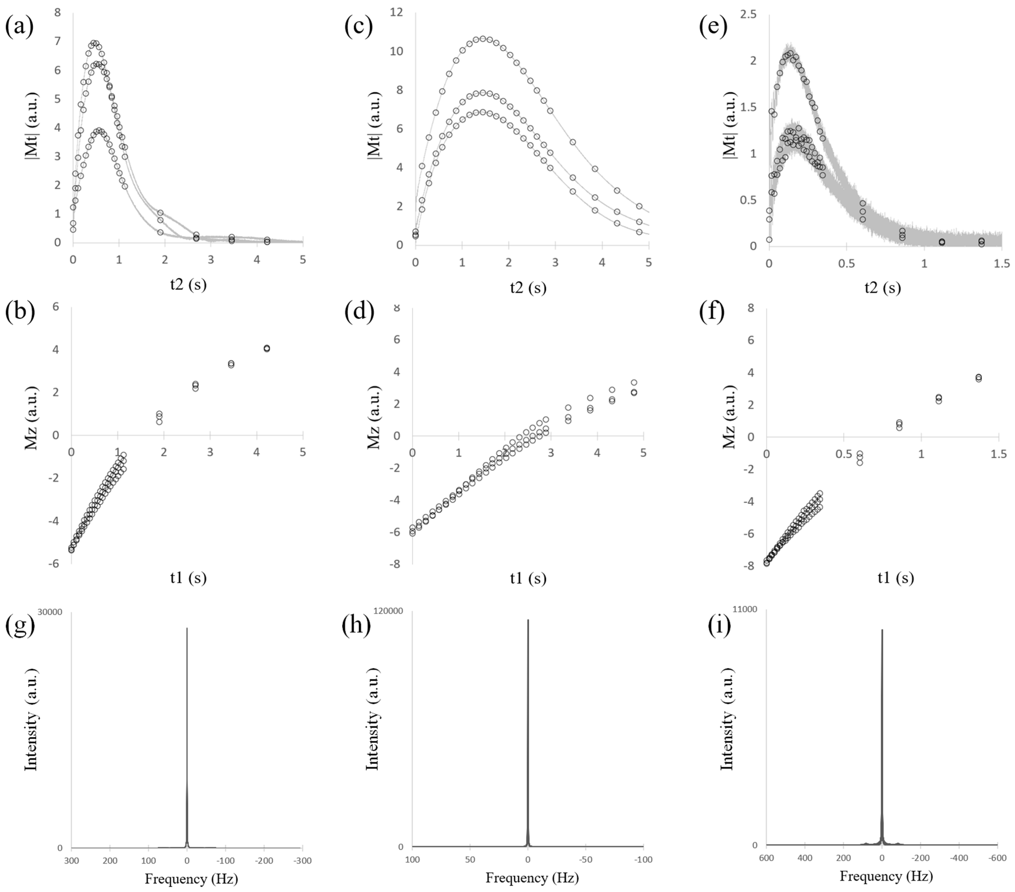
) including the ¹³³Cs, ⁷Li and ³¹P nuclei, we could observe NMR RASER signals on 500 MHz NMR equipment without any special devices. Figure 1 shows measurement results of magnitudes of transverse, $\left|M_t\right|$, and longitudinal, $M_z$, signals planes with respect to time. $\left|M_t\right|$ was not dependent on the phase and $M_z$ was extracted from an inversion recovery experiment. These experimentally measured dynamics with respect to time correspond to $\left|M_t\right|$ and $M_z$ in the theoretical NMR RASER model (Equation (1)). The time variable for transverse magnetization results (Figure 1a,c,e) is labeled as t2, which came from a direct dimension, whereas the time variable for the longitudinal magnetization results (Figure 1b,d,f) is labeled as t1, which came from an indirect dimension. Two pulse sequences for transverse and longitudinal planes were adjusted as they have the same meaning: an elapsed time from an initial state.

Three different experiments for the same ¹³³Cs sample tube exhibited that the magnitudes of transverse magnetization ¹³³Cs were signals of a typical NMR RASER in which signals first increased to its maximum and then decreased toward zero (Figure 1a). All the signals achieved their maximum around 0.6 s and indicated similar dynamics qualitatively. Quantitatively, one signal was observed to be approximately half the magnitude of the other signals due to different shim values. The longitudinal magnetization exhibited recovery to positive magnetization starting from the initial negative states (Figure 1b). For three experiments of the ⁷Li sample, the durations achieving their maximum of transverse magnetization signals were longer and around 1.5 s (Figure 1c). Those of ³¹P were shorter and around 0.15 s (Figure 1e). Similar to the ¹³³Cs results, the dynamics for ⁷Li and ³¹P were qualitatively similar and had approximately twice the maximum magnitude quantitatively. Longitudinal magnetization recovered slower (Figure 1d) and faster (Figure 1f) for ⁷Li and ³¹P, respectively. The transverse magnetization signals for ³¹P had worse signal to noise ratios (Figure 1e). Magnitude spectra for the three samples are shown in Figure 1g–i.

All these results had the following different points of view from that of the NMR RASER results from the ¹H NMR transient RASER [2] experiments. One was that each of our longitudinal magnetization results did not seem to exhibit a hyperbolic tangent signal [31,37] that was found in a normal transient ¹H NMR RASER, but rather seemed to exhibit normal recovery of longitudinal magnetization. Another was that the method for obtaining the NMR RASER (transverse signal) was slightly different. We tried to observe NMR RASER signals with a field gradient method for the elimination of residual transverse magnetization after a 180-degree inversion pulse. The method, however, exhibited lesser signal qualities of the NMR RASER for all of the three samples. Therefore, we did not use the field gradient method; instead, we used a simple inversion pulse improved with an addition of an optimized very short duration, which we called a trigger in this paper, to the length of a 180-degree pulse. This resulted in a continuous and imperfect 180-degree inversion pulse since the trigger was just an addition to the 180-degree pulse. The optimization of trigger lengths was performed on each NMR measurement (see Materials and Methods section). The RASER observed using this method is sometimes quoted as the triggered NMR RASER in the following section of this paper.

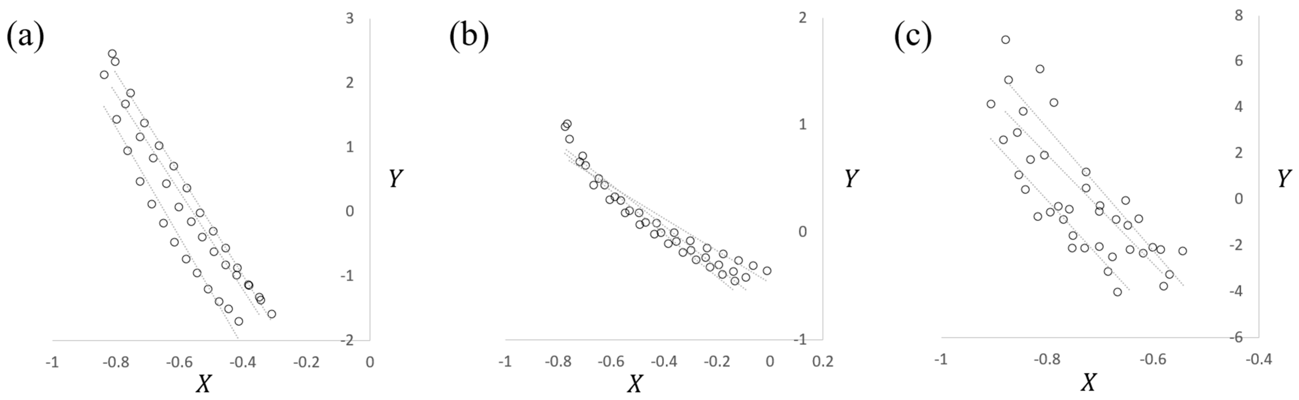
We could conclude that estimations of RD rates for the three heteronuclei, ¹³³Cs, ⁷Li and ³¹P, based on the Bloom model were totally supported (Figure 2). Figure 2 shows the Y vs. X plots in Equation (6) for estimating $R_{rd}$ from the experimental data in Figure 1. The plot shows the rate of transverse magnetization along the Y axis and a fraction of longitudinal magnetization recovery along the X axis. It indicates linearity if experimental observations match the Bloom model. Only a few studies have been published for experimental measurements of RD rates for the heteronuclei.

The result for ¹³³Cs indicated the best linearity among the three heteronuclei (Figure 2a). This slope is an RD rate and is estimated to be 8.0 Hz (

Table 2. Radiation damping rates.

Nucleus	Rrd (Hz)	T2* (s)	T1 (s)
133Cs	8.0 ± 0.5	0.22 ± 0.03	3.3 ± 1.2
7Li	1.8 ± 0.3	1.6 ± 0.5	4.9 ± 0.2
31P	25 ± 1	0.054 ± 0.005	1.3 ± 0.2

). It is affected by different shim currents, and slight shifts in the intercepts, which correspond to $-1/T_2^{\ast }$, among the three experiments were seen. Thus, it is safe to regard estimations as references of $T_2^{\ast }$ in specific shim current conditions, although deviations from the average apparent transverse relaxation time, 0.22 s, were relatively small (Table 2). The apparent transverse relaxation rate of $R_2^{\ast }=1/T_2^{\ast }$ was computed as 4.5 Hz and was smaller than $R_{rd}=$ 8.0 Hz. This was the reason why the net rate of transverse magnetization magnitude at the initial stage was positive, estimated to be 3.5 Hz and why it was increasing. This satisfied the condition of the NMR RASER, where $R_{rd}>R_2^{\ast }$.

The result for ⁷Li indicated that the linearity was limited compared to ¹³³Cs; however, deviations were small among the three experiments (Figure 2b). In the figure, the plots are curved upward, which means that the increase rates of transverse magnetization are slightly faster in the initial stage. This indicated that there was a small discrepancy from the Bloom model between the initial and middle stages of the NMR RASER. The discrepancy was not severe; therefore, we could say that the Bloom model was approximately supported. The $R_{rd}$ was estimated as 1.8 Hz (Table 2). The $R_2^{\ast }$ was computed as 0.63 Hz and it was smaller than the $R_{rd}$ and the difference between them was 1.2 Hz. It was smaller than that of ¹³³Cs, which was the reason why the curves were broad (Figure 1c).

The result for ³¹P indicated that deviations for the three experiments were a large cause of the larger noise in transverse magnetization compared to the other nuclei (Figure 2c). However, the estimated $R_{rd}$ had the smallest relative deviation, 1 Hz ($1/25$ of 25 Hz), compared to the other nuclei (Table 2). Thus, we could say that the Bloom model was also approximately supported. The $R_{rd}$ was estimated as 25 Hz, which was the largest among the three nuclei. The $R_2^{\ast }$ was computed as 19 Hz and the difference of 6 Hz was also the largest among the nuclei.

Using the RD rate constants in Table 2, Equation (4) and the RASER condition in Equation (5), it can be expected that the RASER phenomenon can be observed when the concentrations of ¹³³Cs, ⁷Li and ³¹P are above 4.7, 3.8 and 4.1 mol/L, respectively. We additionally analyzed $T_1$ based on the Bloom model Equation (7). Shortly, linearity and weak linearity for ⁷Li and ¹³³Cs, respectively, were observed, whereas difficulty of analysis caused by noise was found for ³¹P (data not shown). We concluded that estimations of $T_1$ had inaccuracy and thus we only report $T_1$ as the reference estimated values specific for this study (Table 2).

In summary, we concluded that the method in this study that assumed linearity between experimentally measured data based on the Bloom model was adequate for directly estimating $R_{rd}$ from experimentally measured transverse and longitudinal magnetization for all the three nuclei. Estimations of $T_2^{\ast }$ and $T_1$ should be regarded as example reference values specific for individual studies because of their sensitivity to shim currents and due to the strong nonlinearity observed between them, respectively. However, the estimated values of $T_2^{\ast }$ and $T_1$ in this study had relatively small deviations (Table 2); thus, these values must be used as approximations for comparing observed relaxation phenomena for the three nuclei.

5. Discussion

Experimental direct estimations of RD rate constants for the three heteronuclei, ¹³³Cs (spin number I = 7/2), ⁷Li (I = 3/2) and ³¹P (I = 1/2), and observations of (triggered) NMR RASER signals were first achieved. These results are meaningful for further extensions of heteronuclear NMR RASER and spin noise studies. There are only a few studies on the experimental estimation of RD rate constants for the heteronuclei. There are also a small number of studies on the NMR RASER and spin noise, in which RD rates are important, for the heteronuclei. An experimentally direct estimation of RD rate constants for the heteronuclei has ever only been achieved for ³He [12], ¹⁷O [17] and ¹²⁹Xe [19]. The indirect estimation has been achieved for ¹³C [29] and ²⁷Al [14,15]. Heteronuclear NMR RASER signals have been observed for ³He [12,13], ¹³C [16], ¹⁷O [17], ²⁷Al [14,15] and ¹²⁹Xe [13,18,19]. Heteronuclear NMR spin noise signals have been observed only for ¹³C [29]. NMR RASER and spin noise methods have also been extended to MRI methods [49,50,51] for ¹H. Similar MRI methods for the heteronuclei will be possible under experimental conditions in higher values of RD constants.

The method in this study based on the Bloom model was adequate for directly estimating RD rates for all three nuclei samples. These values were not available in the past literature and thus could not be compared. RD rate constants have been published for water ¹H. Our method exhibited RD rate constants for water ¹H in the three 90% H₂O samples used in this study, which were 21, 17 and 19 Hz for the ¹³³Cs, ⁷Li and ³¹P samples, respectively, even though each solution was regarded as a different physicochemical state since the concentration was highly dense. RD rates for water ¹H have been measured in various field strength, samples or estimation methods. Typical examples were 3.2 Hz [38], 19 Hz [20], 25 Hz [25], 31 Hz [43], 37 Hz [5], 40 Hz [25], 50 Hz [28], 76 Hz [40], 91 Hz [37], 130 Hz [40] and 560 Hz [28]. The values obtained using our method for the three samples were within this range. However, we note that the Bloom model is a simple approximated model for the NMR RASER, assuming that there is only one nucleus; thus, no relaxation terms among the nuclei are included. Both ¹³³Cs and ⁷Li possess electric quadrupole moments. The simple measurement spectra obtained with a 90-degree pulse for these samples did not exhibit any splitting or similar features. Instead, an extremely narrow and symmetric on-resonance peak with a line width less than 1 Hz was observed for each of the ¹³³Cs and ⁷Li samples. It can be approximated as a single frequency peak. Therefore, it is reasonable to approximate it using the on-resonance Bloom model in this study.

Based on the Bloom model, although it approximates a real phenomenon, one can interpret that the following two NMR RASER signals are identical. The first one starts from tiny initial transverse magnetization generated with thermal fluctuation after the elimination of residual transverse magnetization with a field gradient. The second one starts from the same size of tiny initial transverse magnetization without a field gradient. Signals of the first type for ¹H have been observed. In the results, residual magnetization after a 180-degree inversion pulse was eliminated with a field gradient and then an amplified NMR RASER signal that started from almost zero was observed [8,25,33,37,45]. This NMR RASER signal can be understood with Equation (1), i.e., the Bloom model. One can obtain $d\left|M_t\right|/dt=0$ by substituting zero for the initial transverse magnetization $\left|M_t\right|\left(0\right)$ in Equation (1); thus, $\left|M_t\right|\left(t\right)=0$. This means that an NMR RASER signal never occurs, provided that both the Bloom model is true and that the initial value of transverse magnetization is completely zero. Provided that $\left|M_t\right|\left(t\right)=0$, one can further see that a solution for longitudinal magnetization, such as $M_z\left(t\right)=M_0\left(1-2 \mathrm{e}\mathrm{x}\mathrm{p}(-t/T_1)\right)$, is just a simple recovery type solution without any RD effect. Therefore, one cannot see a hyperbolic tangent shape [37] that is expected for a longitudinal NMR RASER signal. Provided that the Bloom model is true, we can therefore conclude that initial magnetization in a real experiment cannot be zero and that tiny initial transverse magnetization greater than zero, caused by such thermal fluctuation, must exist. In the NMR RASER results with a field gradient, one can interpret that they observed NMR RASER amplification from a tiny initial value caused by thermal fluctuation that was greater than zero. Such thermal fluctuation is most likely related to spin noise or Nyquist noise [9,18,52]. However, the other author contradicts this claim of Nyquist noise [53]. Observations of amplified NMR signals similar to those in Figure 1a,c,e were also well-known in RD research fields [2,25,31,54] for an incomplete 180-degree inversion pulse or intended initial tiny initial transverse magnetization. The Bloom model was first proposed as an RD model and then utilized for NMR RASER studies. From the above information, one can understand that such a well-known amplified signal from intended initial tiny transverse magnetization in RD phenomenon was a transient (non-sustainable) NMR RASER signal [2]. The Bloom model, however, cannot describe a sustainable NMR RASER. Additions of mathematics to the Bloom model based on an individual experimental device that is utilized as a sustainable mechanism are needed for mathematically describing a sustainable NMR RASER system [4,5,6,7,9,13,15,18,19,46,48].

We note that Z3, Z4 and likely higher-order shimming are important for obtaining a better triggered RASER signal. In this study, we found that a shim change of Z3 and Z4, which had no substantial effect on the quality of a 90-degree spectrum, drastically affects the shape and magnitude of a 180-degree FID, which is an NMR RASER signal. After automated optimization with the Bruker TopShim system, we needed manual optimization in Z3 and Z4 shim currents for more than two hours to obtain one of our results in Figure 1a for the ¹³³Cs sample, whereas the measuring time was performed within 20 s. The shim optimization took about 0.5 h for the ³¹P sample. One should pay attention to the difficulty of shimming for obtaining a better NMR RASER signal shape when similar NMR RASER experiments with this study are needed. NMR RASER signals might have asymmetric distortion or more than one bump under insufficient shim conditions.

The observation of spin noise spectra relies on a high RD rate constant, as has been shown in previous studies [38,41,42]. Measuring RD rates is crucial for both NMR RASER and spin noise research, as estimating the cost of measuring time required to obtain a spin noise spectrum for the nuclei that have not been observed yet is challenging, given the significant time and data size costs involved. The magnitude of a dip spectrum peak in a spin noise spectrum is theoretically proportional to the factor $R_{rd}/(R_{rd}+R_2^{\ast })$, as shown by McCoy et al. [41]. The corresponding values of the factors in this study were 0.6, 0.7 and 0.6 for ¹³³Cs, ⁷Li and ³¹P samples, respectively. Therefore, spin noise spectra for these heteronuclei are expected to be obtained based on this factor, although they have not yet been observed. However, it should be noted that the signal-to-noise ratio, including baseline fluctuations, is also critical for detecting a spin noise peak, in addition to this factor. While this factor is solely dependent on $R_{rd}$ and $R_2^{\ast }$, fluctuations depend on other factors such as temperature and electronic parameters of the probe resonance circuit and preamplifier. Q factors of NMR probe circuits are also important to detect NMR RASER signals and NMR spin noise spectra [30,42]. The Q factors of our NMR probes were roughly estimated as 132, 39 and 31 for ¹³³Cs, ⁷Li and ³¹P measurements, respectively, by using the Bruker wobble curve system.

6. Conclusions

Radio amplification using stimulated emission of radiation (RASER) effects in the NMR can increase NMR signals over time due to a feedback loop between the sample magnetization and the probe coil coupled with radiation damping (RD). Previously, RD rate constants had only been directly observed for the ¹H, ³He, ¹⁷O and ¹²⁹Xe nuclei, and NMR RASER phenomena had been observed for ¹H, ³He, ¹³C, ¹⁷O, ²⁷Al and ¹²⁹Xe. We report that experimental direct measurements of the NMR RASER to determine RD time constants for the three heteronuclei (¹³³Cs (I = 7/2), ⁷Li (I = 3/2) and ³¹P (I = ½)) in a highly concentrated solution from the NMR RASER emissions using a conventional NMR probe. Under conditions where the RD rate exceeds the transverse relaxation rate (i.e., the NMR RASER condition is fulfilled), we recorded both the transverse NMR RASER response to the imperfect inversion and the recovery of longitudinal magnetization. The data were evaluated based on the well-known Bloom model. The on-resonance Bloom model defines the dynamics of transverse and longitudinal magnetization. Therefore, we could estimate RD rate constants by calculating slopes after sampling a set of measured NMR data sets. Based on the results, we could estimate RD rate constants of 8.0, 1.8 and 25 Hz for ¹³³Cs, ⁷Li and ³¹P, respectively.

Many applied NMR researchers are familiar with the RD phenomenon but are often unaware of the NMR RASER, despite the fact that these two phenomena are the same. In this study, we employed the well-known Bloom model, commonly used in various NMR RASER studies, to observe the transient NMR RASER phenomenon corresponding to the initial amplification stage for the first time. While the sustainable NMR RASER phenomena have not been observed for the ¹³³Cs, ⁷Li and ³¹P nuclei, our results confirm the occurrence of the first amplification stage. If one can provide continuous negative longitudinal magnetization using techniques such as DNP, sustainable NMR RASER observations may become possible for these three nuclei. Additionally, estimating RASER conditions relies on the observation of RD rate constants, and the method proposed in this study can be applied to observe RD rate constants for the other nuclei as well.