Simulation and Theory of Classical Spin Hopping on a Lattice

Abstract

The behavior of spin for incoherently hopping carriers is critical to understand in a variety of systems such as organic semiconductors, amorphous semiconductors, and muon-implanted materials. This work specifically examined the spin relaxation of hopping spin/charge carriers through a cubic lattice in the presence of varying degrees of energy disorder when the carrier spin is treated classically and random spin rotations are suffered during the hopping process (to mimic spin–orbit coupling effects) instead of during the wait time period (which would be more appropriate for hyperfine coupling). The problem was studied under a variety of different assumptions regarding the hopping rates and the random local fields. In some cases, analytic solutions for the spin relaxation rate were obtained. In all the models, we found that exponentially distributed energy disorder led to a drastic reduction in spin polarization losses that fell nonexponentially.

1. Introduction

Spin relaxation of carriers has garnered much interest in the past few decades due to the prospect of spin electronic or spintronic devices that use spin functionality in addition to charge functionality. However, most work has been concentrated on band transport [1,2,3,4,5]. Less effort has been expended on the spin relaxation of localized electron spins where charge transport occurs via incoherent hopping motion. Noncrystalline, organic semiconductors have recently seen a surge in interest [6,7,8,9,10,11,12] as spintronic candidates due to their small spin–orbit coupling and expected long spin lifetimes of 10${}^{-5}$–10${}^{-7}$ s [13]. Within the field of spin chemistry, spin relaxation plays a role in radical pair reactions [14], which has applications varying from organic electronic devices [15] to avian navigation [16]. Localized spin relaxation also plays a role in transport through disordered crystalline semiconductors [17,18].

Spin relaxation of hopping spins has an older genesis: it was first studied in relation to muon spectroscopy [19,20,21,22,23,24]. The technique has seen much application in the study of magnetic materials. Muon spin spectroscopy is used to study kinetic isotope effects in chemical reactions [25]. The method involves positively charged polarized (spin 1/2) muons, ${\mu }^{+}$, being implanted into a material. The interaction of the muon spin with local magnetic moments allows the technique to be an excellent probe of magnetic properties. The muon’s lifetime is only 2.1970 μs, after which it decays into two neutrinos and a positron. The utility of the mechanism is due to the positron being emitted preferentially along the direction of its parent’s spin. By detecting emitted positrons, the spin evolution of the implanted muon is revealed. When that evolution is impacted by spin interactions with the host material, temporal muon decay measurements may yield information about the host material; time scales that can be probed by this technique range from picoseconds to microseconds. Due to the positron emission being sensitive to magnetic interactions, probing spontaneous magnetic fields in magnetic materials was an early application of muon spectroscopy [26]. In dielectrics, semiconductors, and organic compounds, a low-energy muon can form a stable state with an electron: muonium. Muonium offers access to hydrogen-like states in these materials and can be especially beneficial in the study of chemical reactions where muonium serves as a radical [27].

Information from muon spectroscopy is obtained from the measured polarization of the implanted muons. For static fields, stationary muon spins experience a distribution of environmental magnetic fields whose ensemble average yields the measured response. When muons diffuse throughout the host, the fields fluctuate, which alters the spin decay function of the ensemble [24]. Calculations of the polarization in time yield information on the fields, as well as the hopping diffusion of the muons. Figure 1a shows how the classical spin rotation is coherent at each location, but then abruptly changes when an incoherent hop occurs; at the new location, the evolution is again coherent, and the process repeats until the spin polarization decays to zero. Since the spin is rotated while situated at a site, we call this an intrasite process of spin relaxation. The intersite process involves the spin rotating during the hopping process itself, while the spin is stationary when sitting on a site. Intrasite processes dominate the polarization functions of muon spectroscopy and therefore have been well studied for many decades [19,28,29]. Previous studies have shown that quantum and classical calculations of spin diffusion length agree well [8,30]. The time to hop, $1/k$, varies widely from system to system. As discussed later, the time is strongly dependent on energetic disorder. Times can be as short as femtoseconds [31].

Intersite spin evolution, depicted in Figure 1b, occurs when the spin experiences some rotation (or flip in a quantum picture) during the transition between two localizing centers. This type of mechanism is similar to the process of spin relaxation by spin–orbit interactions in organic semiconductors [12,32,33,34,35,36]. Here, we investigated in depth a classical model of spin relaxation from a spin–orbit-type interaction.

2. Theory

In this section, an analytic theory of classical spin relaxation is reviewed for intrasite mechanisms [34].

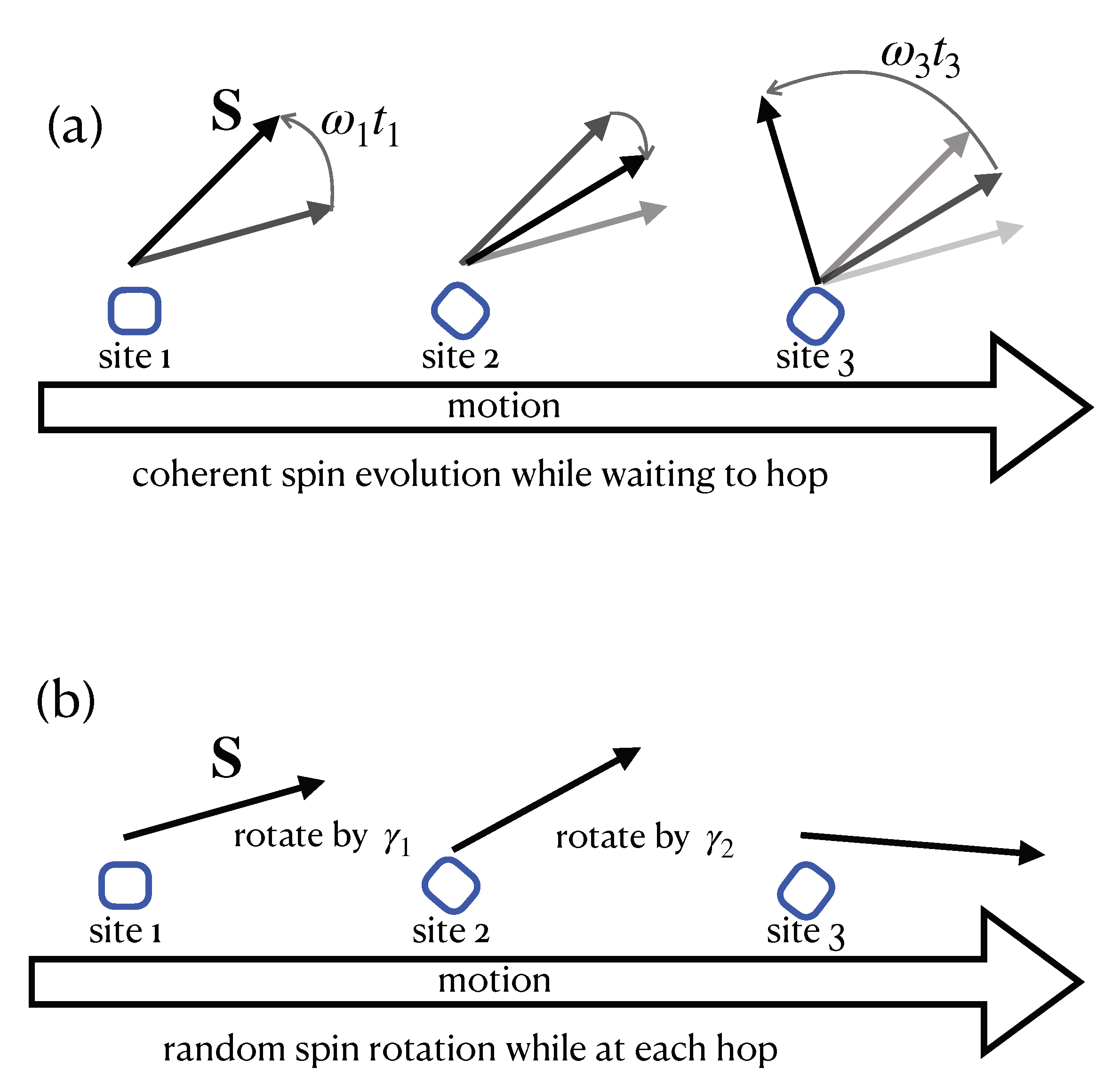
2.1. Spin Evolution

The unit vector, $\mathit{S}$, is a classical electron spin, which in an arbitrary uniform, static magnetic field, $\mathit{B}$, has a precessional frequency $-\mathbf{\omega }=-|{\gamma }_e|\mathbf{B}/2\approx {\mu }_{B}B\mathbf{n}/ħ$, where ${\gamma }_e=g{\mu }_B/ħ$, $\mathit{n}$ is the unit vector of $\mathit{B}$, and the Lande factor for spin is taken to be two. The evolution of $\mathit{S}$ is described by the following equation:

$$\frac{d\mathit{S}\left(t\right)}{dt}=-\mathbf{\omega }\times \mathit{S}\left(t\right)=\mathsf{\Omega }\mathit{S}\left(t\right),$$

(1)

where $\mathsf{\Omega }$ is the skew-symmetric matrix:

$$\begin{array}{ccc}\hfill \mathsf{\Omega }& =& -\omega \widehat{\mathsf{\Omega }}=-\left(\begin{array}{ccc}0& -{\omega }_z& {\omega }_y\\ {\omega }_z& 0& -{\omega }_x\\ -{\omega }_y& {\omega }_x& 0\end{array}\right)\hfill \\ & \equiv & -\omega \left(\begin{array}{ccc}0& -cos\theta & sin\theta sin\varphi \\ cos\theta & 0& -sin\theta cos\varphi \\ -sin\theta sin\varphi & sin\theta cos\varphi & 0\end{array}\right).\hfill \end{array}$$

(2)

Intrasite spin relaxation (hopping independent) was not considered here. The solution to Equation (1) is:

$$\mathit{S}\left(t\right)=e^{\mathsf{\Omega }t}{\mathit{S}}_0\equiv \widehat{\mathbf{R}}\left(t\right){\mathit{S}}_0,$$

(3)

where ${\mathit{S}}_0$ is the initial spin vector and $\mathit{R}$ is the following rotation matrix:

$$\widehat{\mathbf{R}}\left(t\right)=\widehat{\mathbf{1}}+sin\omega t\widehat{\mathsf{\Omega }}+2{sin}^2\frac{\omega t}{2}\widehat{\mathsf{\Omega }}\widehat{\mathsf{\Omega }}$$

(4)

which is equivalent to this vectorial expression [37]:

$$\mathit{S}\left(t\right)=({\mathit{S}}_0·\mathit{n})\mathit{n}+\left\{{\mathit{S}}_0-({\mathit{S}}_0·\mathit{n})\mathit{n}\right\}cos\omega t+\left[\left\{{\mathit{S}}_0-\left({\mathit{S}}_0·\mathit{n}\right)\mathit{n}\right\}\times \mathit{n}\right]sin\omega t.$$

(5)

If $\mathbf{\omega }=0$, there is no spin evolution at a site, so $\widehat{\mathbf{R}}\left(t\right)=\widehat{\mathbf{1}}$ and $\mathit{S}\left(t\right)={\mathit{S}}_0$. Spin relaxation occurs when carriers hop between different sites with random local magnetic fields. This was explored in the context of hyperfine interactions and inhomogeneous g-factors in previous articles [12,34]. Intrasite spin evolution will be ignored from hereon out.

The focus here is on an alternate spin relaxation mechanism where spin rotations occur between hops—the so-called intersite process of spin relaxation. The spin changes abruptly at each hop instead of coherently evolving while fixed at a localizing center. The spin, after a single hop, is updated as:

$$\mathit{S}(t+dt)={\widehat{\mathbf{T}}}_{\gamma }{\mathit{S}}_0$$

(6)

where:

$${\widehat{\mathbf{T}}}_{\gamma }=\widehat{\mathbf{1}}+sin\gamma \widehat{\mathsf{\Omega }}+2{sin}^2\frac{\gamma }{2}\widehat{\mathsf{\Omega }}\widehat{\mathsf{\Omega }}$$

(7)

or:

$$\mathit{S}(t+dt)=({\mathit{S}}_0·\mathit{n})\mathit{n}+\left\{{\mathit{S}}_0-({\mathit{S}}_0·\mathit{n})\mathit{n}\right\}cos\gamma +\left[\left\{{\mathit{S}}_0-\left({\mathit{S}}_0·\mathit{n}\right)\mathit{n}\right\}\times \mathit{n}\right]sin\gamma .$$

(8)

The process can be repeated to model the evolution of the spin. For a single spin, the spin will randomly walk on the unit sphere as the spin hops to various sites with random $\gamma \mathit{n}$ fields. Later in this article, we will simulate this process for an ensemble of spins. However, analytic theories can be devised for the ensemble if appropriate approximations are made. This is the subject of the next section.

2.2. Strong Collision Approximation

We used an approximation known as the strong-collision approximation [38]. The approximation is characterized by the following assumptions: (1) local field changes are abrupt and not slow at each hop (non-Gaussian); (2) local fields during each hop are uncorrelated from any previous hop (Markovian).

With the strong-collision approximation, the theory of continuous-time random walks [39,40] can be used to calculate the polarization functions of hopping carrier spins. Two important functions of continuous-time random walk theory are the survival probability, $\mathsf{\Phi }\left(t\right)$, and the wait time distribution, $\psi \left(t\right)$. $\mathsf{\Phi }\left(t\right)$ is the probability that a random walker starting on a site at $t=0$ has not hopped by time t. $\psi \left(t\right)$ is the probability distribution from which the hopping times are chosen. The two quantities are related by:

$$d\mathsf{\Phi }\left(t\right)/dt=-\psi \left(t\right),\mathsf{\Phi }\left(t\right)={\int }_t^{\infty }\psi \left(t^{\prime }\right)d{t}^{\prime }=1-{\int }_0^t\psi \left(t^{\prime }\right)d{t}^{\prime }.$$

(9)

The polarization of spins that have not hopped is then ${\mathit{P}}_0\left(t\right)=\mathsf{\Phi }\left(t\right){\mathit{S}}_0$, since only those spins that have “survived” on their initial site contribute the polarization of stationary spins.

The polarization of spins that have hopped exactly one time by time t is ${\mathit{P}}_1\left(t\right)={\widehat{\mathbf{R}}}_1\left(t\right){\mathit{S}}_0$, where:

$${\widehat{\mathbf{R}}}_1\left(t\right)=\langle {\int }_0^t\mathsf{\Phi }(t-t^{\prime }){\widehat{\mathbf{T}}}_{\gamma ,1}\psi \left(t^{\prime }\right)d{t}^{\prime }\rangle ={\int }_0^t\mathsf{\Phi }(t-t^{\prime })\langle {\widehat{\mathbf{T}}}_{\gamma ,1}\rangle \psi \left(t^{\prime }\right)d{t}^{\prime }$$

(10)

where ${\widehat{\mathbf{R}}}_1\left(t\right)$ is the rotation matrix for the sub-ensemble of spins that have rotated one time by time t. This equation is interpreted term-by-term going from right to left: the probability of making a single hop in the interval $d{t}^{\prime }$ is $\psi \left(t^{\prime }\right)d{t}^{\prime }$; the rotation of the spin as it hops one time, due to the intersite process, is ${\widehat{\mathbf{T}}}_{\gamma ,n}$, where n is the nth hop in the sequence of hops; once the hop is completed, the spin remains at the new site according to the survival probability. Since there is an ensemble of spins of which many will hop a single time within the interval t, we must integrate over the possible hopping time $d{t}^{\prime }$. Lastly, the angular brackets denote an average over the angular coordinates of the ${\widehat{\mathbf{T}}}_{\gamma ,1}$ rotation matrix Equation (7), which yields:

$$\langle {\widehat{\mathbf{T}}}_{\gamma ,1}\rangle =\widehat{\mathbf{1}}+2{sin}^2\frac{\gamma }{2}\langle \widehat{\mathsf{\Omega }}\widehat{\mathsf{\Omega }}\rangle =\widehat{\mathbf{1}}-\frac{4}{3}{sin}^2\frac{\gamma }{2}\widehat{\mathbf{1}}.$$

(11)

The magnitude of the rotation angle, $\gamma$, is held constant for the time being. The cumulative rotation matrix for spins that have hopped twice is:

$$\begin{array}{ccc}\hfill {\widehat{\mathbf{R}}}_2\left(t\right)& =& \langle {\int }_0^{t}d{t}^{\prime }{\int }_0^{t^{\prime }}d{t}^{″}\mathsf{\Phi }(t-t^{\prime }){\widehat{\mathbf{T}}}_{\gamma ,2}\psi (t^{\prime }-t^{″}){\widehat{\mathbf{T}}}_{\gamma ,1}\psi \left(t^{″}\right)\rangle \hfill \\ & =& {\langle {\widehat{\mathbf{T}}}_{\gamma ,2}\rangle }^2{\int }_0^{t}d{t}^{\prime }{\int }_0^{t^{\prime }}d{t}^{″}\mathsf{\Phi }(t-t^{\prime })\psi (t^{\prime }-t^{″})\psi \left(t^{″}\right)\hfill \end{array}$$

(12)

where the angular averaging of the two rotations, ${\widehat{\mathbf{T}}}_{\gamma ,1}$ and ${\widehat{\mathbf{T}}}_{\gamma ,2}$, is independent since there is no correlation between local fields; the two average rotation matrices are also equal; we then denote their average as $\langle {\widehat{\mathbf{T}}}_{\gamma ,1}\rangle =\langle {\widehat{\mathbf{T}}}_{\gamma ,2}\rangle \equiv {\widehat{\mathbf{T}}}_{\gamma }$. The polarization of these two-hoppers is ${\mathit{P}}_2\left(t\right)={\widehat{\mathbf{R}}}_2\left(t\right){\mathit{S}}_0$. The generalization to higher order hops is straightforward, which leads to a total polarization $\mathit{P}\left(t\right)={\sum }_{n=0}^{\infty }{\widehat{\mathbf{R}}}_n\left(t\right){\mathit{S}}_0$. The net polarization function becomes tractable by Laplace transformations and the convolution theorem.

Analytic solutions are obtained by Laplace transforming the rotation matrices. For instance:

$${\widetilde{\widehat{\mathbf{R}}}}_0\left(s\right)=\tilde{\mathsf{\Phi }}\left(s\right)\widehat{1},{\widetilde{\widehat{\mathbf{R}}}}_1\left(s\right)={\widehat{\mathbf{T}}}_{\gamma }\tilde{\mathsf{\Phi }}\left(s\right)\tilde{\psi }\left(s\right),{\widetilde{\widehat{\mathbf{R}}}}_2\left(s\right)={\widehat{\mathbf{T}}}_{\gamma }^2\tilde{\mathsf{\Phi }}\left(s\right)\tilde{\psi }{\left(s\right)}^2$$

(13)

feed into $\tilde{\mathit{P}}\left(s\right)={\sum }_{n=0}^{\infty }{\widetilde{\widehat{\mathbf{R}}}}_n\left(s\right)·{\mathit{S}}_0$, which is a geometric series summable to:

$$\tilde{\mathit{P}}\left(s\right)=\frac{\tilde{\mathsf{\Phi }}\left(s\right)}{1-{\widehat{\mathbf{T}}}_{\gamma }\tilde{\psi }\left(s\right)}{\mathit{S}}_0$$

(14)

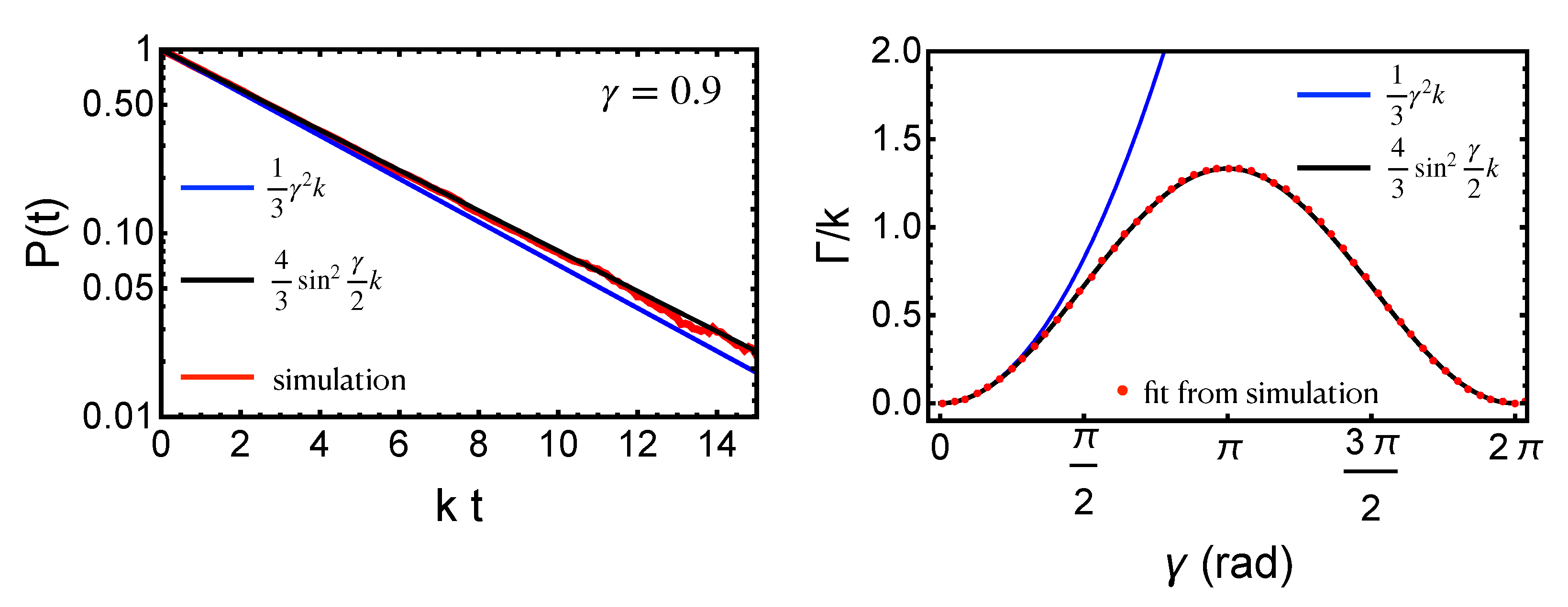
2.3. Non-Disordered Model

A simple example of the theory is demonstrated by using a exponential wait time distribution, $\psi \left(t\right)=k{e}^{-kt}$, where k is the average hopping rate. The relevant quantities feeding into Equation (14) are $\tilde{\psi }\left(s\right)=k/(k+s)$ and $\tilde{\mathsf{\Psi }}\left(s\right)=1/(k+s)$, which yield first:

$$\tilde{\mathit{P}}\left(s\right)=\frac{1/(k+s)}{1-{\widehat{\mathbf{T}}}_{\gamma }k/(k+s)}{\mathit{S}}_0$$

(15)

which is reduced to:

$$\tilde{\mathit{P}}\left(s\right)=\frac{1}{s+k(1-{\widehat{\mathbf{T}}}_{\gamma })}{\mathit{S}}_0=\frac{1}{s+\frac{4}{3}k{sin}^2\frac{\gamma }{2}}{\mathit{S}}_0.$$

(16)

The desired polarization function in time is ascertained by the inverse Laplace transform to be:

$$\mathit{P}\left(t\right)=e^{-\frac{4}{3}k{sin}^2\frac{\gamma }{2}t}{\mathit{S}}_0.$$

(17)

When the spin rotation angle $\gamma$ is small, the polarization function is:

$$\mathit{P}\left(t\right)=e^{-\frac{1}{3}k{\gamma }^{2}t}{\mathit{S}}_0.$$

(18)

A comparison of the full polarization function, the approximate polarization function suitable for small rotation angles, and the multiple trapping simulations (to be described later) are displayed in Figure 2. The relaxation rate’s $k{\gamma }^2$ dependence can be correlated with a quantum spin model for spin–orbit-induced spin relaxation, where $\gamma$ is interpreted as a spin admixture parameter instead of a rotation angle. First principle calculations of $\gamma$ for a common organic semiconductors yield 10${}^{-2}$ –10${}^{-4}$ [32].

2.4. Hopping Models

The spin relaxation of hopping spins is modeled in two ways. The first is Multiple Trapping (MT), where each hops is completely uncorrelated from previous hops. The advantage of this model is the ability to obtain analytic solutions. The disadvantage is that in a real system, hops are in fact correlated, which means the random fields giving rise to relaxation are correlated. The Multiple Hopping (MH) model accounts for these correlations. We used Monte Carlo methods to simulate both models.

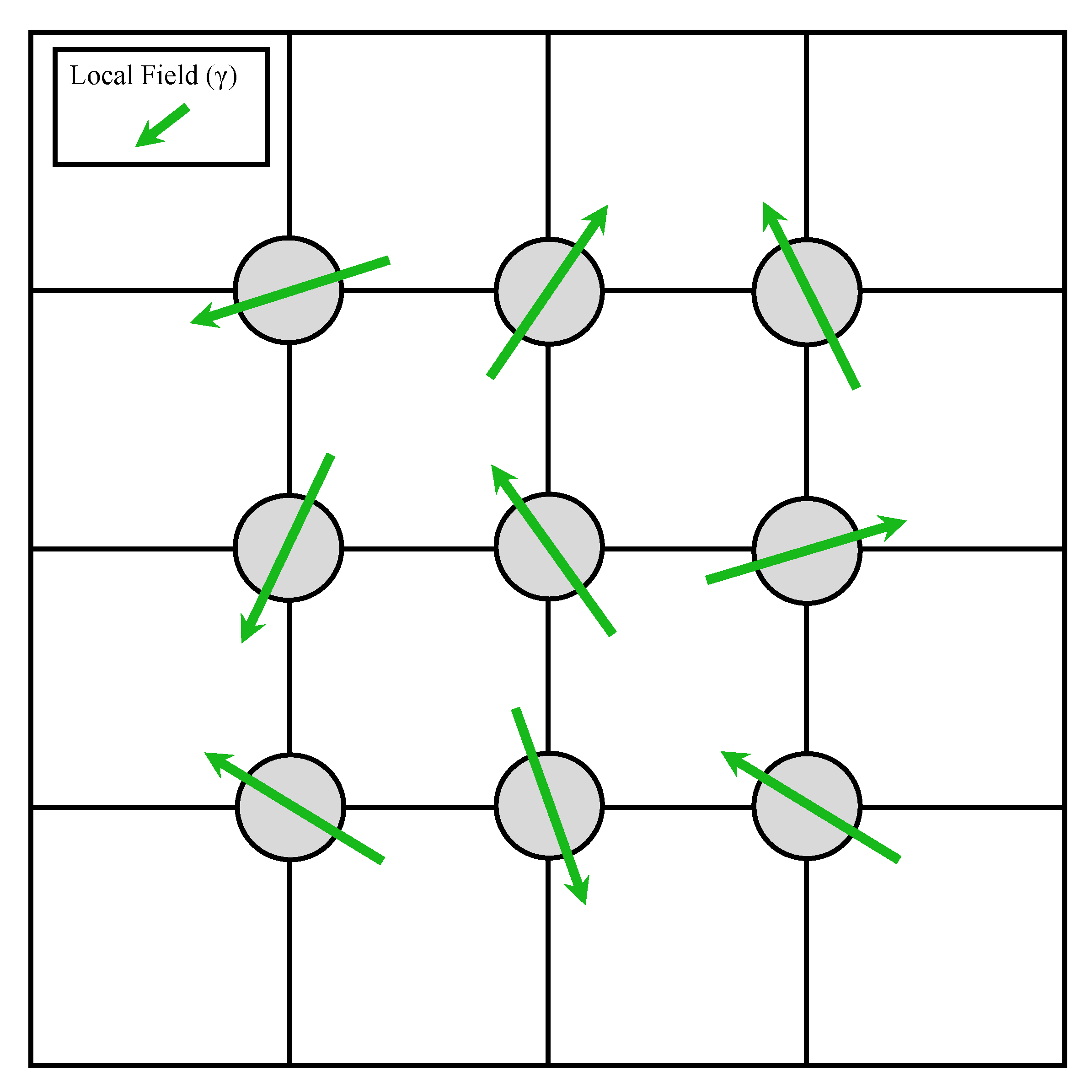
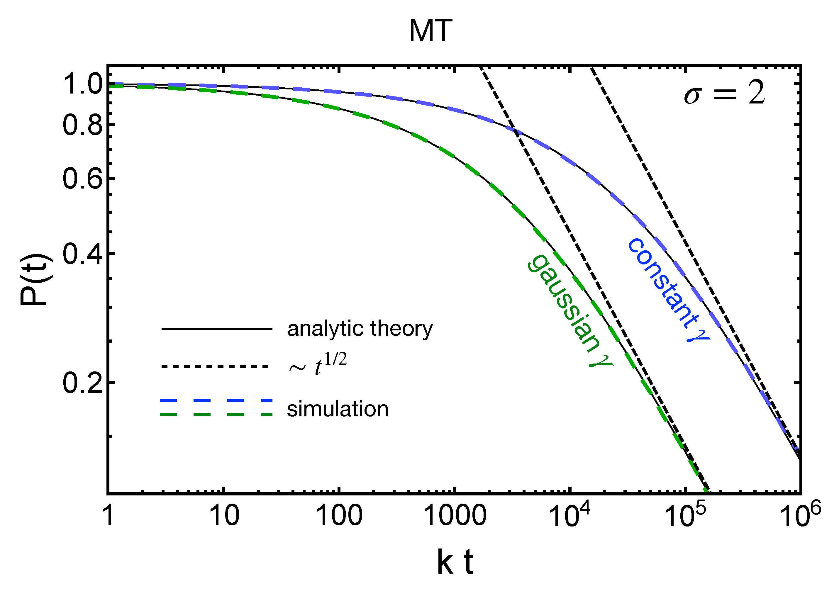
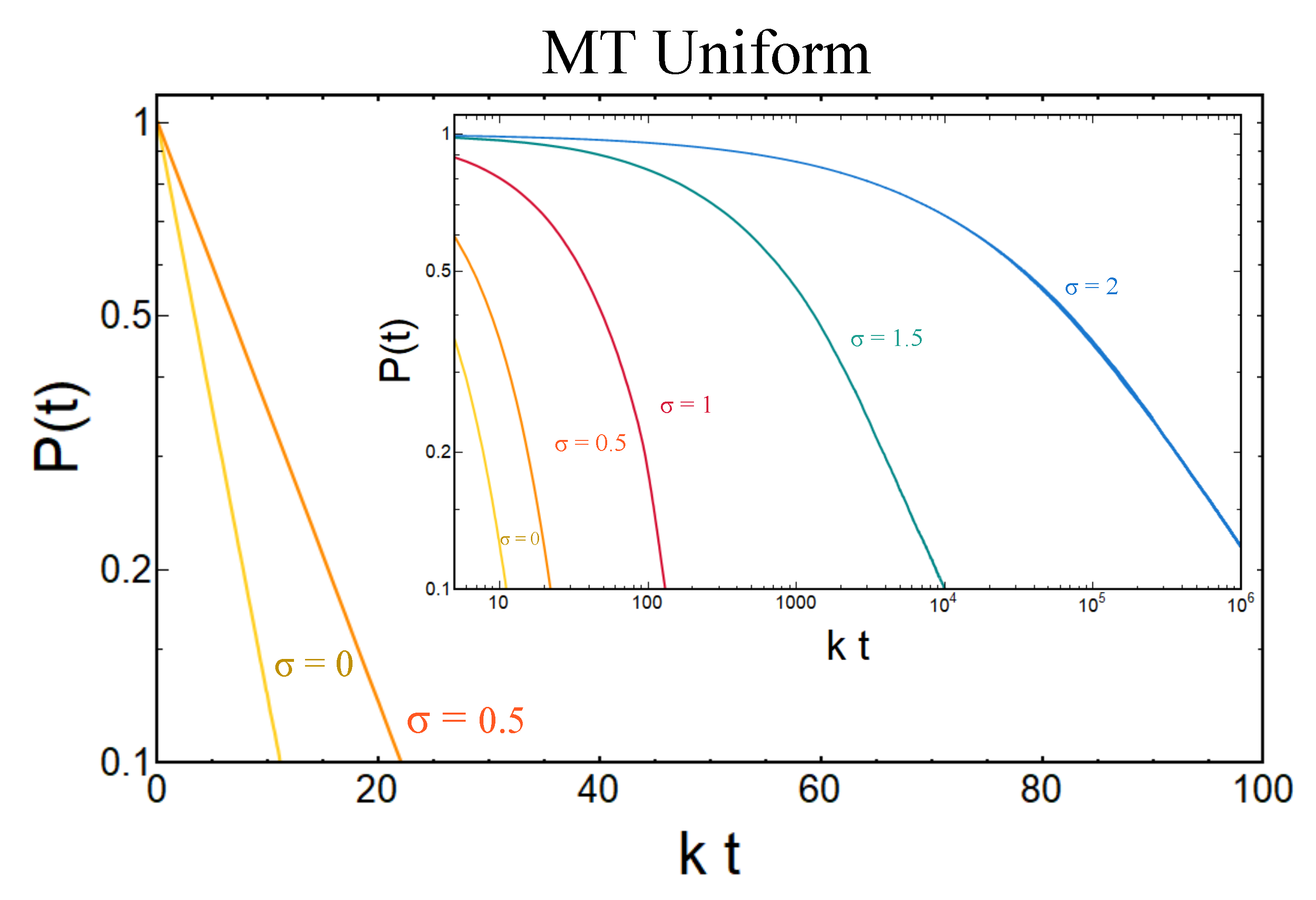
2.5. Multiple Trapping Model

Realistic wait time distributions, appropriate for amorphous and organic semiconductors, are harder to handle than what was treated in Section 2.3. The two aforementioned disordered systems are typically characterized by an exponential density of states and a Gaussian density of states, respectively. The width of the Gaussian is typically taken to be on the order of tenths of an electron volt in organic semiconductors [41]. The Multiple Trapping model (MT) constructs wait time distributions $\psi \left(t\right)=k\left(\epsilon \right)e^{-k\left(\epsilon \right)t}$ from hopping rates that are of the form of trap release rates, $k\left(\epsilon \right)=k_0{e}^{\epsilon /k_{B}T}$, where $\epsilon$ is the trap energy and is distributed according to the density of states. The energy levels are uncorrelated between hops. The strong-collision approximation is still assumed, so there is no correlation in rotational fields either. For an exponential density of states, $g_e\left(\epsilon \right)={\left(k_B{T}_0\right)}^{-1}exp(\epsilon /k_B{T}_0)$, $\psi \left(t\right)$ is described by ${\int }_{-\infty }^0{g}_e\left(\epsilon \right)k\left(\epsilon \right)e^{-k\left(\epsilon \right)t}d\epsilon$ or in Laplace space as:

$$\tilde{\psi }\left(s\right)={\int }_{-\infty }^{0}d\epsilon g_e\left(\epsilon \right)\frac{k\left(\epsilon \right)}{s+k\left(\epsilon \right)}={\int }_{-\infty }^{0}dx{e}^x\frac{k_0{e}^{x/\alpha }}{s+k_0{e}^{x/\alpha }},$$

(19)

with $x=\epsilon /k_B{T}_0$ and $\alpha =T/T_0$. The result can be written as a hypergeometric function:

$$\tilde{\psi }\left(s\right)=\frac{k_0\alpha }{s+\alpha s}{}_2{F}_1(1,1+\alpha ,2+\alpha ,-k_0/s).$$

(20)

The long time, or asymptotic, behaviors of $\psi \left(t\right)$ and $\mathsf{\Phi }\left(t\right)$ are of interest; they are determined to be [34]:

$$\psi (t\to \infty )\sim \frac{t^{-\alpha -1}}{k_0^{\alpha }},\mathsf{\Phi }(t\to \infty )\sim \frac{t^{-\alpha }}{k_0^{\alpha }}.$$

(21)

The polarization at any time can be ascertained by the numerical Laplace transform inversion [42] of Equation (14) [43,44]. However, in the long-time case, asymptotic analysis determines [34]:

$$P\left(t\right)=\frac{n\pi \alpha }{\mathsf{\Gamma }(1-\alpha )}\frac{1}{k_0^{\alpha }}\frac{1}{{\gamma }^2}csc\left(\pi \alpha \right)t^{-\alpha }$$

(22)

which demonstrates an algebraic decay of spin polarization. $n=3$ for $\gamma$ distributed with a constant magnitude over a sphere and $n=1$ for a randomly directed Gaussian $\gamma$.

For a Gaussian density of states, $g_g\left(\epsilon \right)={(2\pi {\sigma }^2)}^{-1/2}exp(-{\epsilon }^2/2{\sigma }^2)$, the problem is less analytically and computationally tractable as neither pure exponential nor power law behavior are observed for finite $\sigma /k_{B}T$ [8,45].

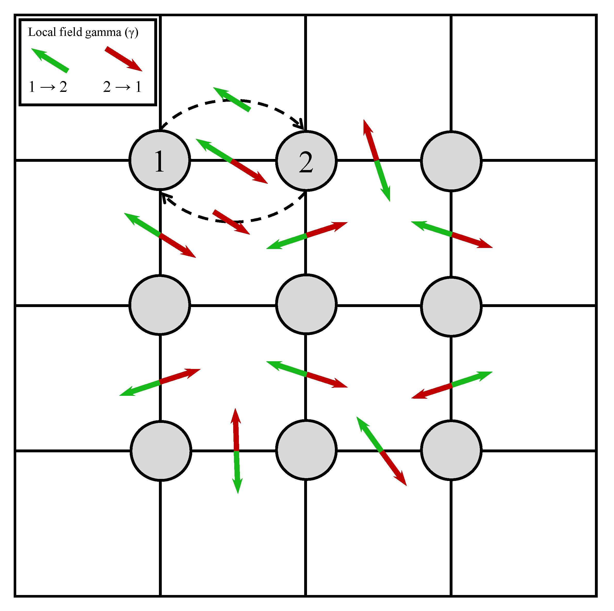
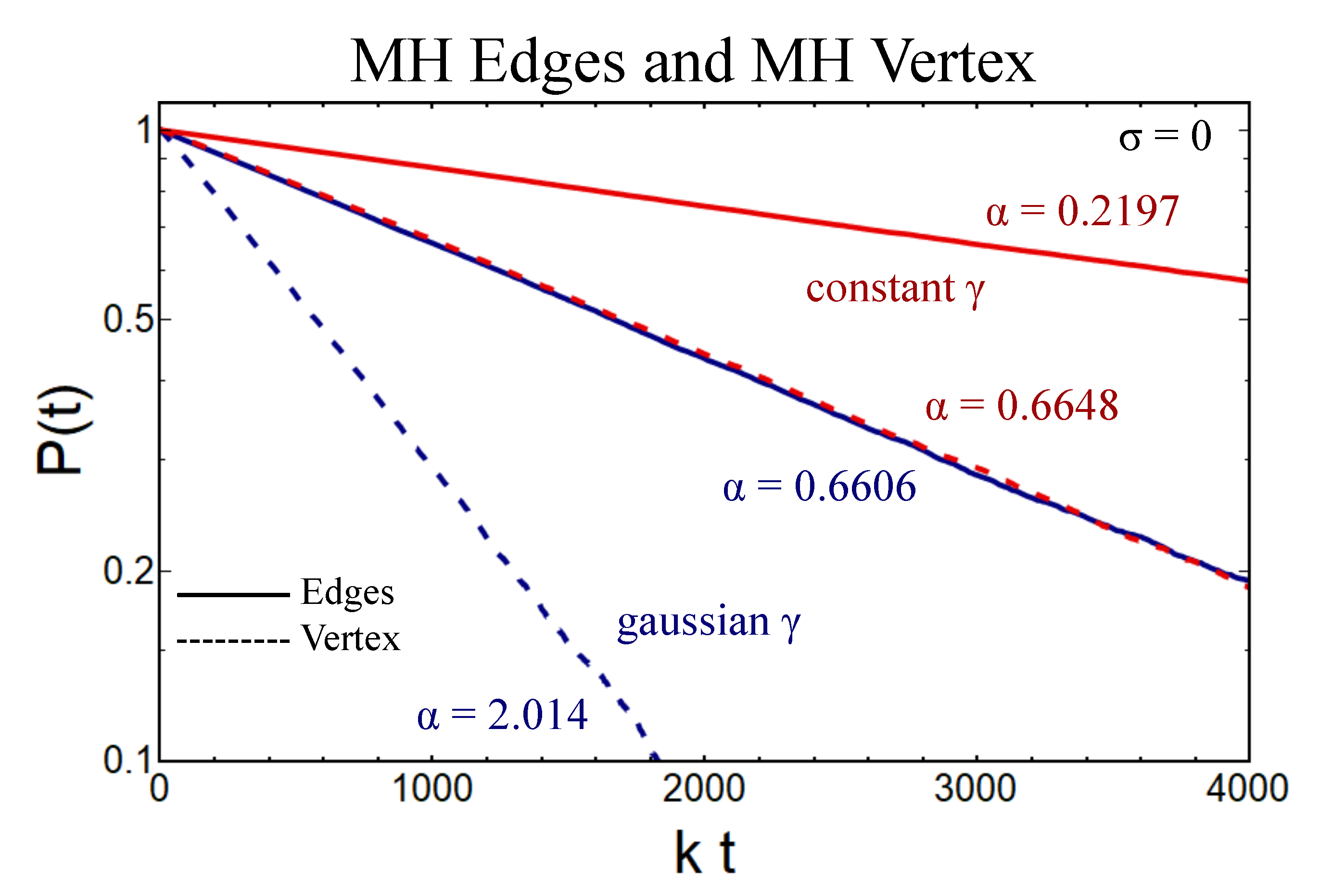
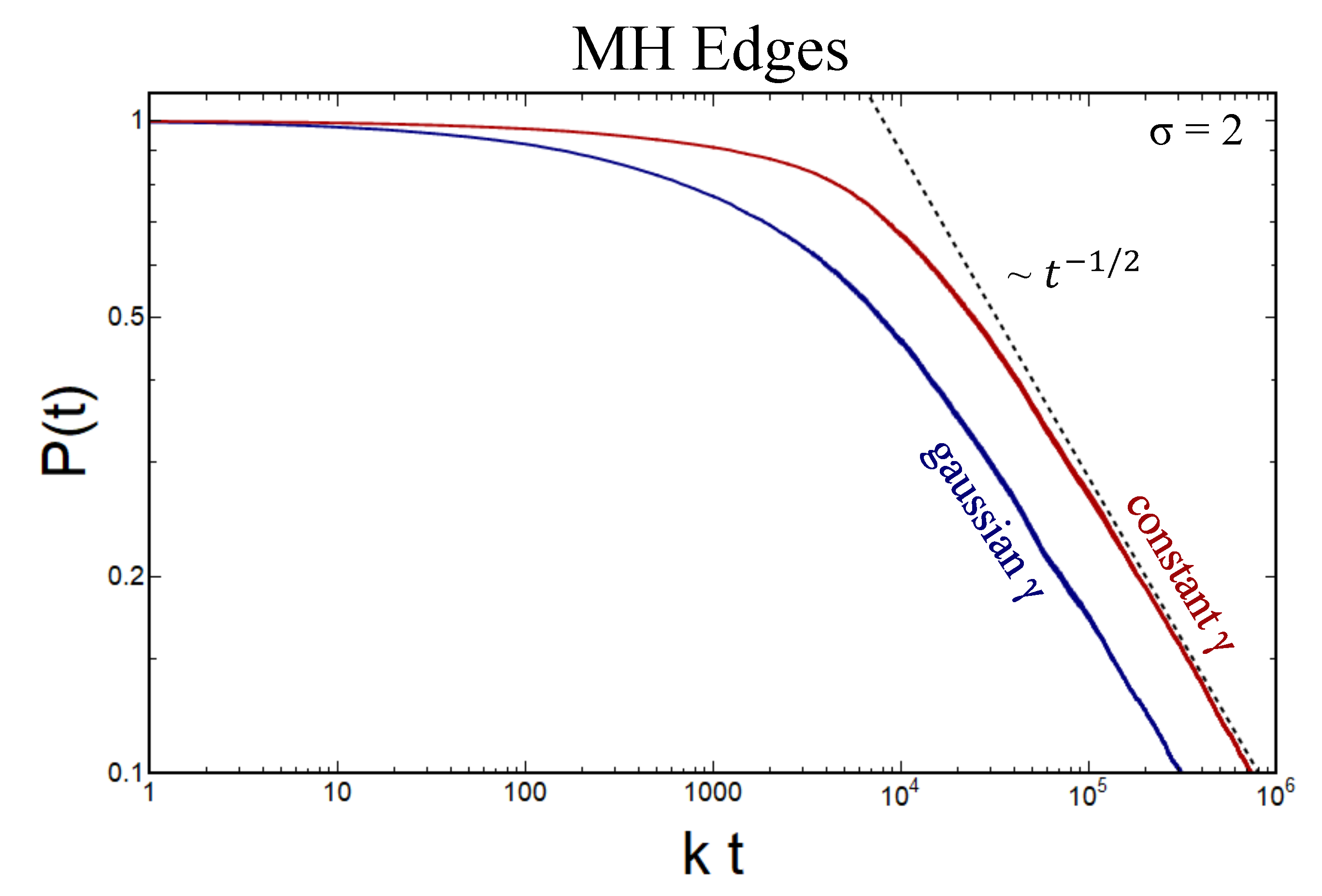
2.6. Multiple Hopping Model

The MT model treats each hop as an independent trap release with release rate $k\left(\epsilon \right)=k_0{e}^{\epsilon /k_{B}T}$. MT ignores correlations between sites, which would cause the hopping to not follow the carrier release from distribution sites with some density of states. For example, two sites lying near in energy and space would allow rapid back-and-forth hopping before the charge carrier escapes the dyad. Therefore, MT is inappropriate in general, but is useful due to its simplicity and the availability of analytic solutions to some problems.

To address more realistic hopping, we adopted a Monte Carlo approach where charge hopping and concomitant spin evolution are tracked on a cubic lattice where the rate of hopping from site i to site j is determined by the Miller–Abrahams rates:

$$k_{ij}=\left\{\begin{array}{cc}{k}_0,\hfill & \mathrm{if}{\epsilon }_i\ge {\epsilon }_j,\hfill \\ k_0{e}^{({\epsilon }_i-{\epsilon }_j)/k_{B}T},\hfill & \mathrm{if}{\epsilon }_i<{\epsilon }_j.\hfill \end{array}\right.$$

(23)

Each site on the lattice is assigned a fixed energy drawn from the chosen density of states (either the delta function, exponential, or Gaussian). The field vector responsible for rotating the spin is $\gamma \mathit{n}$. Later on, different assignations for $\gamma$ are discussed. Spin carriers were injected randomly onto the lattice of sites. The spin of each carrier was sampled at a chosen time interval and averaged over many different configurations of the disorder (typically 10,000–50,000). A single disorder configuration possesses a fixed landscape of site energies and local fields.

Various models for the local fields, $\gamma$, can be employed. Below, we describe two models for the correlation of the fields between sites (applicable only to MH) and two models of the local field vector (applicable to either MT or MH).

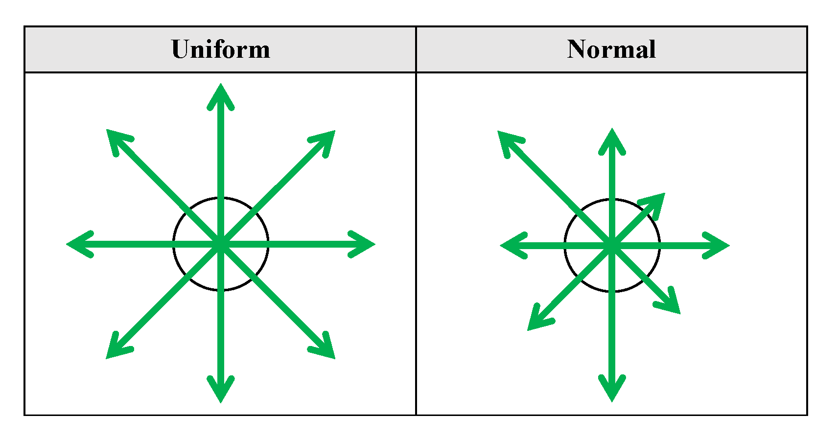
2.6.1. Local Field Correlations

The previous site is always “forgotten” after each hop in the MT model, so models of site correlations only apply to the MH model. Two models were employed: the vertex and edge local fields models.

Vertex local fields: Each site possesses a single local field vector $\gamma$, which exerts a torque on the spin hopping to that site, as shown in Figure 3. This model was employed in [12,34].

Edge local fields (commuting): The local field exists between two nearest neighbor sites. The local field for a forward hop is opposite that of a backward hop. Therefore, a spin that undergoes a forward–backward hop combination ends up with its initial spin state as shown in Figure 4. This model mimics spin–orbit interactions for sub-barrier carrier motion [35].

2.6.2. Local Field Magnitude

Two different models of the local field magnitude were employed (demonstrated in Figure 5): (1) the magnitude was constant (the direction was random); (2) the magnitude was drawn from the Gaussian distribution (the direction was again random).

Constant local fields: Each local field has a fixed magnitude, but a random direction, such that the rotation angle is $\mathsf{\Gamma }\mathit{n}$, where $\mathsf{\Gamma }$ is constant. This leads to a spin relaxation function $\mathit{P}\left(t\right)=e^{-\frac{1}{3}k{\mathsf{\Gamma }}^{2}t}{\mathit{S}}_0$.

Gaussian local fields: If each component of the rotational vector $\mathsf{\Gamma }\mathit{n}$ is isotropically, normally distributed with width $\gamma$, then in the small-angle approximation for $\mathsf{\Gamma }$, the relaxation rates change to ${\gamma }^{2}k$ such that $\mathit{P}\left(t\right)=e^{-k{\gamma }^{2}t}{\mathit{S}}_0$.

Details on the implementation of these models are described in Section 5.

3. Results

Now, the results from the aforementioned simulations are presented. First, the results using zero disorder ($\sigma =0$) are shown, and then, the results for finite disorder (using an exponential density of states) are displayed.

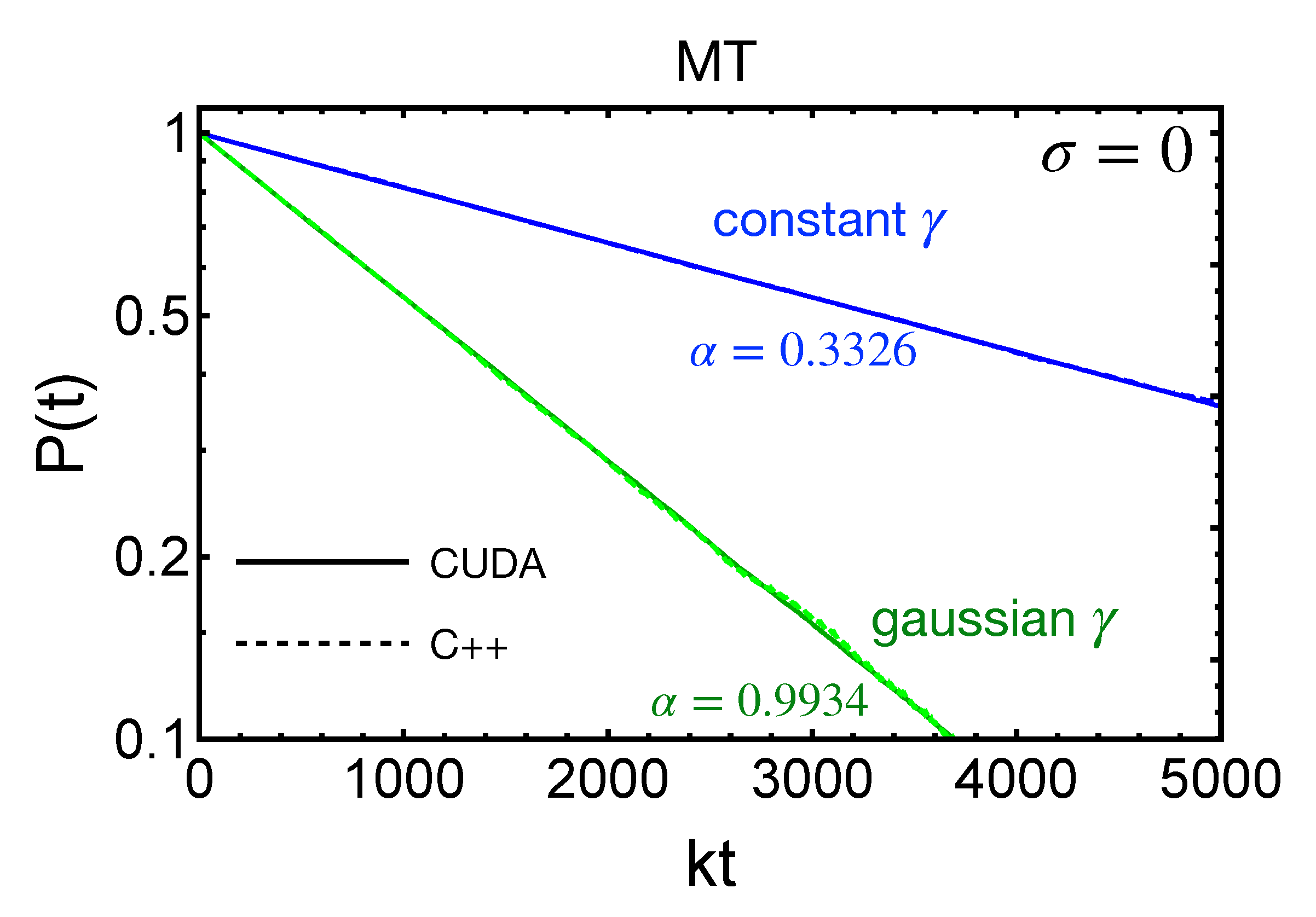
3.1. Zero Disorder

Simulations of MT and MH using each of the previously described models are demonstrated in Figure 6 and Figure 7. Exponential fits for nondisordered simulations were carried out with the function:

$$P_{\mathrm{fit}}\left(t\right)=P_0{e}^{-\alpha {\gamma }^{2}kt}$$

(24)

where $P_0$ and $\alpha$ serve as fitting parameters.

Table 1. Rational approximations for the values of $\alpha$, found computationally, when $\sigma =0$. Values preceded by “∼” denote rationalizations of numerical results (in other words, these values are not derived analytically).

α	MT	MH
Gaussian	1	–
Gaussian-vertex	–	2.014∼2
Gaussian-edge	–	2/3
constant	1/3	–
constant-vertex	–	0.6606∼2/3
constant-edge	–	2/9

shows the values of $\alpha$ obtained for each model. The MT values were derived from the theory presented earlier in this article.

In view of all the MH simulations in the figures below, one can readily understand why the edges model led to slower spin relaxation: since to-and-fro hops commuted, such hops led to no spin losses where every hop in the vertex model had the potential of incurring a random spin rotation.

An interesting finding demonstrated in Table 1 is that the MH-edges rate is found to be 2/3 the MT rate (for both field magnitude models). We can understand the factor of $2/3$ in the following way. In MT, all six hopping directions lead to a spin rotation (and hence, contribute to spin relaxation). For the MH-edges model, only five hopping options contribute to spin relaxation; the sixth option is a return to the spin’s previous site, which will actually suppress the spin relaxation due to the assumed commutation of back-and-forth hops. By compiling the fraction of hops that lead to relaxation or reduce relaxation, on a cubic lattice, we have $\frac{5}{6}(+1)+\frac{1}{6}(-1)=\frac{4}{6}=\frac{2}{3}$. In general, with coordination number q, the relaxation suppression fraction is $\frac{q-1}{q}(+1)+\frac{1}{q}(-1)=\frac{q-2}{q}$, which we confirmed for the square lattice.

3.2. Finite Disorder

Figure 8, Figure 9 and Figure 10 demonstrate the role nonzero disorder ($\sigma >0$) plays in the spin polarization functions. Figure 8 is the MT model with $\sigma =2$. The thin black lines are the analytic results from inverse Laplace transforms of Equation (20). The linear dashed lines are the analytic approximation at longer times given by Equation (22). The key features, when $\sigma >1$, are that the polarization function decays algebraically at long times no matter the model being used (however, an exponential density of states was assumed here).

The much slower algebraic relaxation (as opposed to exponential) was due to the high-disorder regime of $\sigma >1$. Spin rotations only occurred during hops, and large disorder means that carriers would fall into deep energy states and take a long time to hop out. Since relaxation requires hops, the relaxation function follows the same trend as the survival probability function.

Figure 9 shows a similar behavior for the MH-edges model, and we found the MH-vertex model (not shown) to be qualitatively identical as well.

Figure 10 is again the MT model, but this time with several different values for the disorder parameter $\sigma$. The relaxation function is exponential for $\sigma <1$ and algebraic for $\sigma >1$. These functional dependencies on $\sigma$ correspond to the notions of non-dispersive and dispersive transport known to the amorphous semiconductor community.

4. Discussion

The simulations presented above modeled the instantaneous rotation of a classical carrier spin as it hopped across a lattice. While our model was a classical approximation to a quantum mechanical, the motivation was that this type of model should qualitatively pick up some features of hopping-induced spin–orbit spin relaxation, which is believed to be responsible for the spin losses in some amorphous and organic semiconductors. In this section, we discuss the aspects and shortcomings of our classical model, as well as future directions this work will take.

4.1. Evaluating the Models

In terms of capturing the relevant physics, the MH model is superior due to the accounting of correlations during hops. The edges version of MH is most applicable to underbarrier motion undergoing a spin–orbit interaction [35]. The vertex version of MH is most suitable for overbarrier hopping transport, where one would not expect commuting spin rotations between adjacent sites.

Determining which of all the models presented here (MT, MH, vertex, edges, Gaussian, constant) are governing a particular system is difficult due to the uncertainty in the parameters ($\gamma$, k) for a given system. This can be seen for the following reasons: (1) if $\sigma =0$, all models predict spin relaxation rates, $\alpha {\gamma }^{2}k$ with $\alpha$ differing by order unity; (2) if $\sigma >0$, all models predict algebraic spin decay ∼$t^{-1/\sigma }$.

The predicted ∼${\gamma }^{2}k$ dependence for spin relaxation was used in [46] to fit experimental electron spin resonance measurements in undoped amorphous silicon [47,48] and hydrogenated amorphous silicon [49,50]. While these amorphous systems are disordered (which entails algebraic decay), the $\sim {\gamma }^{2}k$ dependence for the line shape width may be due to resonance experiments picking up short-time exponential dynamics. A better comparison with the theory presented here, to probe the influence of strong disorder, would require experiments performed using time-resolved electron spin resonance.

Time-of-flight experiments clearly demonstrate the role of disorder in charge transport (so-called dispersive transport) [51,52]; however, extending this method to spin transport is nontrivial, and the authors are not aware of any experiments of this type.

4.2. Shortcomings of the Classical Spin Model

Consider a simple model atom in the 2p state, where $p_z$ has an energy $\mathsf{\Delta }$ below that of $p_x$ and $p_y$. For the spin–orbit Hamiltonian, $H_{so}=\xi \mathbf{L}·\mathbf{S}$, perturbation theory yields doubly degenerate eigenstates:

$$|+\rangle =|p_z\uparrow \rangle +\frac{\xi }{2\mathsf{\Delta }}|(p_x+i{p}_y)\downarrow \rangle$$

(25)

$$|-\rangle =|p_z\downarrow \rangle -\frac{\xi }{2\mathsf{\Delta }}|(p_x-i{p}_y)\uparrow \rangle$$

(26)

and a spin–orbit energy shift of $-{\xi }^2/\mathsf{\Delta }$. $|+\rangle$ and $|-\rangle$ are pseudospin states: since $\xi /\mathsf{\Delta }$ is small, the $|+\rangle$ pseudospin state is mostly $|\uparrow \rangle$ with a small component of $|\downarrow \rangle$.

Spin–orbit coupling mixes up- and down-spin spin states, which entails that spin is not conserved. The hopping integral between two sites i and j is spin independent, but since the pseudospin states $|+\rangle$ and $|-\rangle$ are admixtures of up and down states, there is a finite probability for transitions between $|+\rangle$ and $|-\rangle$ states during hopping events.

If one takes the local fields to signify spin–orbit interactions, we can contrast the classical model with quantum models of carriers hopping between sites experiencing spin–orbit interactions [32,33,36]. Due to the spin–orbit Hamiltonian not commuting with the spin operators, spin is not conserved during hops. Typically, in an organic semiconductor (e.g., Alq3), the spin–orbit interaction is weak, such that many spin-conserving hops may take place before a spin flip. The classical spin model presented herein describes the spin relaxation as a more continuous process, where small spin rotations occur at each hop and the accrual of such rotations leads to relaxation. The quantum model as described by [32,33,36] is inconsistent with the underbarrier motion modeled by MH-edges [35]. The deviation of the classical MH model with the quantum model (for simplicity, we assumed no disorder) is starkest in lower dimensional hopping systems, where commuting hops are assumed by the edges model. The commutation of oppositely directed hops suppresses spin relaxation, while we do not expect such a dramatic suppression in the quantum spin model (since spin flips occur probabilistically, there would be no spin flip reversals when returning to a site). A detailed study of the quantum model awaits our further focus.

5. Materials and Methods

Calculations were carried out in Python, C++, and CUDA. These three languages were chosen in order to confirm each other and also to parallelize the computations. MH codes initialized a classical spin vector and then allowed the spin to randomly walk over a cubic (for 3D simulations) lattice (typically 80${}^3$, which proved to be far beyond where finite-size effects would be observed) according to the Miller–Abrahams hopping rates. The spin vector would be sampled every $\mathsf{\Delta }t$. Many thousands of spins were evolved in this manner, and their vector at every $\mathsf{\Delta }t$ would then be averaged to find the average spin decay function. When disorder was present, each run would randomize the site energies according to the density of states. The MT code operated in a similar fashion, except that the activation energy at each hop was randomly drawn according to the density of states. In this manner, each hop is completely uncorrelated from the previous hops.

6. Conclusions

For the first time, we provided a systematic treatment of intersite classical spin relaxation processes for hopping carrier spins. The variety of models examined, while classical, carried enough features to give insight into what may occur for a hopping quantum mechanical spin experiencing spin–orbit interactions during the hopping processes. Given a specific amount of disorder, the classical models do not deviate enough from each other to adequately distinguish between them since important spin–orbit and hopping parameters are not known to high precision. Future efforts will be to study spin relaxation from hopping using a fully quantum mechanical spin–orbit interaction.

References

- Yafet, Y. g Factors and Spin-Lattice Relaxation of Conduction Electrons. Solid State Phys. 1963, 14, 2–98. [Google Scholar]
- Meier, F.; Zachachrenya, B.P. Optical Orientation: Modern Problems in Condensed Matter Science; North-Holland: Amsterdam, The Netherlands, 1984; Volume 8. [Google Scholar]
- Ziese, M.; Thornton, M.J. (Eds.) Spin Electronics; Lecture Notes in Physics; Springer: Berlin/Heidelberg, Germany, 2001; Volume 569. [Google Scholar]
- Awschalom, D.D.; Samarth, N.; Loss, D. (Eds.) Semiconductor Spintronics and Quantum Computation; Springer: Berlin/Heidelberg, Germany, 2002. [Google Scholar]
- Samarth, N. An Introduction to Semiconductor Spintronics. Solid State Phys. 2004, 58, 1–72. [Google Scholar]
- Dediu, V.; Murgia, M.; Matacotta, F.C.; Taliani, C.; Barbanera, S. Room temperature spin polarized injection in organic semiconductor. Solid State Commun. 2002, 122, 181–184. [Google Scholar] [CrossRef]
- Xiong, Z.H.; Wu, D.; Vardeny, Z.V.; Shi, J. Giant magnetoresistance in organic spin-valves. Nature 2004, 427, 821–824. [Google Scholar] [CrossRef] [PubMed]
- Bobbert, P.A.; Wagemans, W.; Oost, F.W.A.; Koopmans, B.; Wohlgenannt, M. Theory for spin diffusion in disordered organic semiconductors. Phys. Rev. Lett. 2009, 102, 156604. [Google Scholar] [CrossRef] [Green Version]
- Nguyen, T.D.; Hukic-Markosian, G.; Wang, F.; Wojcik, L.; Li, X.G.; Ehrenfreund, E.; Vardeny, Z.V. Isotope effect in spin response of π-conjugated polymer films and devices. Nat. Mater. 2010, 9, 345. [Google Scholar] [CrossRef]
- Baker, W.J.; Keevers, T.L.; Lupton, J.M.; McCamey, D.R.; Boehme, C. Slow hopping and spin dephasing of Coulombically bound polaron pairs in an organic semiconductor at room temperature. Phys. Rev. Lett. 2012, 108, 267601. [Google Scholar] [CrossRef] [PubMed] [Green Version]
- Rybicki, J.; Lin, R.; Wang, F.; Wohlgenannt, M.; He, C.; Sanders, T.; Suzuki, Y. Tuning the performance of organic spintronic devices using x-ray generated traps. Phys. Rev. Lett. 2012, 109, 076603. [Google Scholar] [CrossRef] [Green Version]
- Harmon, N.J.; Flatté, M.E. Distinguishing spin relaxation mechanisms in organic semiconductors. Phys. Rev. Lett. 2013, 110, 176602. [Google Scholar] [CrossRef]
- Tian, Q.; Xie, S. Spin injection and transport in organic materials. Micromachines 2019, 10, 596. [Google Scholar] [CrossRef] [Green Version]
- Schulten, K.; Wolynes, P.G. Semiclassical description of electron spin motion in radicals including the effect of electron hopping. J. Chem. Phys. 1978, 68, 3292. [Google Scholar] [CrossRef]
- Deotare, P.B.; Chang, W.; Hontz, E.; Congreve, D.N.; Shi, L.; Reusswig, P.D.; Modtland, B.; Bahlke, M.E.; Lee, C.K.; Willard, A.P.; et al. Nanoscale transport of charge-transfer states in organic donor?acceptor blends. Nat. Mater. 2015, 14, 1130–1134. [Google Scholar] [CrossRef]
- Ritz, T.; Wiltschko, R.; Wiltschko, R.; Hore, P.J.; Rodgers, C.T.; Stapput, K.; Thalau, P.; Timmel, C.R.; Wiltschk, W. Magnetic Compass of Birds Is Based on a Molecule with Optimal Directional Sensitivity. Biophys. J. 2009, 96, 3451. [Google Scholar] [CrossRef] [PubMed] [Green Version]
- Cochrane, C.J.; Lenahan, P.M. Zero-field detection of spin dependent recombination with direct observation of electron nuclear hyperfine interactions in the absence of an oscillating electromagnetic field. J. Appl. Phys. 2012, 112, 123714. [Google Scholar] [CrossRef]
- Harmon, N.J.; McMillan, S.R.; Ashton, J.P.; Lenahan, P.M.; Flatté, M.E. Coherent Detection of Single or Few Defects. IEEE Trans. Nucl. Sci. 2020, 67, 1669–1673. [Google Scholar] [CrossRef]
- Kehr, K.W.; Honig, G.; Richter, D. Stochastic theory of spin depolarization of muons diffusing in the presence of traps. Z. Phys. B 1978, 32, 49. [Google Scholar] [CrossRef]
- Czech, R.K. Spin depolarization for one-dimensional random walk. Phys. Rev. Lett. 1984, 53, 3–6. [Google Scholar] [CrossRef]
- Czech, R. Spin depolarization by random walks in lattice gases. J. Chem. Phys. 1989, 91, 2506. [Google Scholar] [CrossRef]
- Czech, R. Number of distinct sites visited by random walks in lattice gases. J. Chem. Phys. 1989, 91, 2498. [Google Scholar] [CrossRef]
- Smilga, V.; Belousov, Y.M. The Muon Method in Science; Nova Science Publishers: New York, NY, USA, 1994. [Google Scholar]
- Yaouanc, A.; de Rèotier, P.D. Muon Spin Rotation, Relaxation, and Resonance; Oxford University Press: New York, NY, USA, 2011. [Google Scholar]
- Ghandi, K.; Clark, I.P.; Lord, J.S.; Cottrell, S.P. Laser-muon spin spectroscopy in liquids: A technique to study the excited state chemistry of transients. Phys. Chem. Chem. Phys. 2007, 9, 353–359. [Google Scholar] [CrossRef]
- Foy, M.L.G.; Heiman, N.; Kossler, W.J.; Stronach, C.E. Precession of Positive Muons in Nickel and Iron. Phys. Rev. Lett. 1973, 30, 1064–1067. [Google Scholar] [CrossRef]
- Reid, I.D.; Azuma, T.; Roduner, E. Surface-adsorbed free radicals observed by positive-muon avoided-level-crossing resonance. Nature 1990, 345, 328–330. [Google Scholar] [CrossRef]
- Kubo, R.; Tomita, K. A General Theory of Magnetic Resonance Absorption. J. Phys. Soc. Jpn. 1954, 9, 888–919. [Google Scholar] [CrossRef]
- Abragam, A. Principles of Nuclear Magnetism; Oxford Science Publications: Oxford, UK, 1961. [Google Scholar]
- Adhikari, P.; Harmon, N.J. Spin diffusion in organic semiconductors. 2021; unpublished. [Google Scholar]
- Landi, A.; Borrelli, R.; Capobianco, A.; Velardo, A.; Peluso, A. Hole Hopping Rates in Organic Semiconductors: A Second-Order Cumulant Approach. J. Chem. Theory Comput. 2018, 14, 1594–1601. [Google Scholar] [CrossRef] [PubMed]
- Yu, Z.G. Spin-orbit coupling, spin relaxation, and spin diffusion in organic solids. Phys. Rev. Lett. 2011, 106, 106602. [Google Scholar] [CrossRef] [PubMed]
- Yu, Z.G. Spin-orbit coupling and its effects in organic solids. Phys. Rev. B 2012, 85, 115201. [Google Scholar] [CrossRef] [Green Version]
- Harmon, N.J.; Flatté, M.E. Spin Relaxation in Materials Lacking Coherent Charge Transport. Phys. Rev. B 2014, 90, 115203. [Google Scholar] [CrossRef] [Green Version]
- Shumilin, A.V.; Kabanov, V.V. Kinetic equations for hopping transport and spin relaxation in a random magnetic field. Phys. Rev. B 2015, 92, 014206. [Google Scholar] [CrossRef] [Green Version]
- McMillan, S.R.; Harmon, N.J.; Flatté, M.E. Steric Paper. 2021; unpublished. [Google Scholar]
- Merkulov, I.A. Electron spin relaxation by nuclei in semiconductor quantum dots. Phys. Rev. B 2002, 65, 1–8. [Google Scholar] [CrossRef] [Green Version]
- Hayano, R.S.; Uemura, Y.J.; Imazato, J.; Yamazaki, T.; Kubo, R. Zero and low field spin relaxation studied by positive muons. Phys. Rev. B 1979, 20, 850. [Google Scholar] [CrossRef]
- Montroll, E.W.; Weiss, G.H. Random walks on lattices. II. J. Math. Phys. 1965, 6, 167. [Google Scholar] [CrossRef]
- Klafter, J.; Sokolov, I.M. First Steps in Random Walks; Oxford University Press: New York, NY, USA, 2011. [Google Scholar]
- Baranovskii, S.D. Theoretical description of charge transport in disordered organic semiconductors. Phys. Stat. Solidi B 2014, 251, 487. [Google Scholar] [CrossRef]
- GWR and Talbot Numerical Inverse Laplace Transform Methods. Available online: http://library.wolfram.com/infocenter/ (accessed on 10 March 2021).
- Valkó, P.P.; Abate, J. Comparison of sequence accelerators for the Gaver method of numerical Laplace transform inversion. Comput. Math. Appl. 2004, 48, 629. [Google Scholar] [CrossRef] [Green Version]
- Abate, J.; Valkó, P.P. Multi-precision Laplace Transform inversion. Int. J. Numer. Meth. Eng. 2004, 60, 979. [Google Scholar] [CrossRef]
- Hartenstein, B.; Bassler, H.; Jakobs, A.; Kehr, K.W. Comparison between multiple trapping and multiple hopping transport in random medium. Phys. Rev. B 1996, 54, 8574. [Google Scholar] [CrossRef] [PubMed]
- Harmon, N.J.; Flatté, M.E. Organic magnetoresistance from deep traps. J. Appl. Phys. 2014, 116, 043707. [Google Scholar] [CrossRef] [Green Version]
- Voget-Grote, U.; Stuke, J.; Wagner, H. Electron spin resonance of amorphous silicon. AIP Conf. Proc. 1976, 31, 91. [Google Scholar]
- Movaghar, B.; Schweitzer, L. ESR and conductivity in amorphous germanium and silicon. Phys. Stat. Solidi B 1977, 80, 491. [Google Scholar] [CrossRef]
- Dersch, H.; Stuke, J.; Beichler, J. Electron Spin Resonance of Doped Glow-Discharge Amorphous Silicon. Phys. Stat. Solidi B 1981, 105, 265. [Google Scholar] [CrossRef]
- Dersch, H.; Stuke, J.; Beichler, J. Temperature dependence of ESR spectra of doped a-Si:H. Phys. Stat. Solidi B 1981, 107, 307. [Google Scholar] [CrossRef]
- Pfister, G.; Scher, H. Dispersive (non-Gaussian) transient transport in disordered solids. Adv. Phys. 1978, 27, 747. [Google Scholar] [CrossRef]
- Borsenberger, P.M.; Pautmeier, L.T.; Bassler, H. Nondispersive-to-dispersive charge-transport transition in disordered molecular solids. Phys. Rev. B 1992, 46, 12145. [Google Scholar] [CrossRef] [PubMed]