Unraveling Nanoscale Magnetic Ordering in Fe3O4 Nanoparticle Assemblies via X-rays

 , and
, and 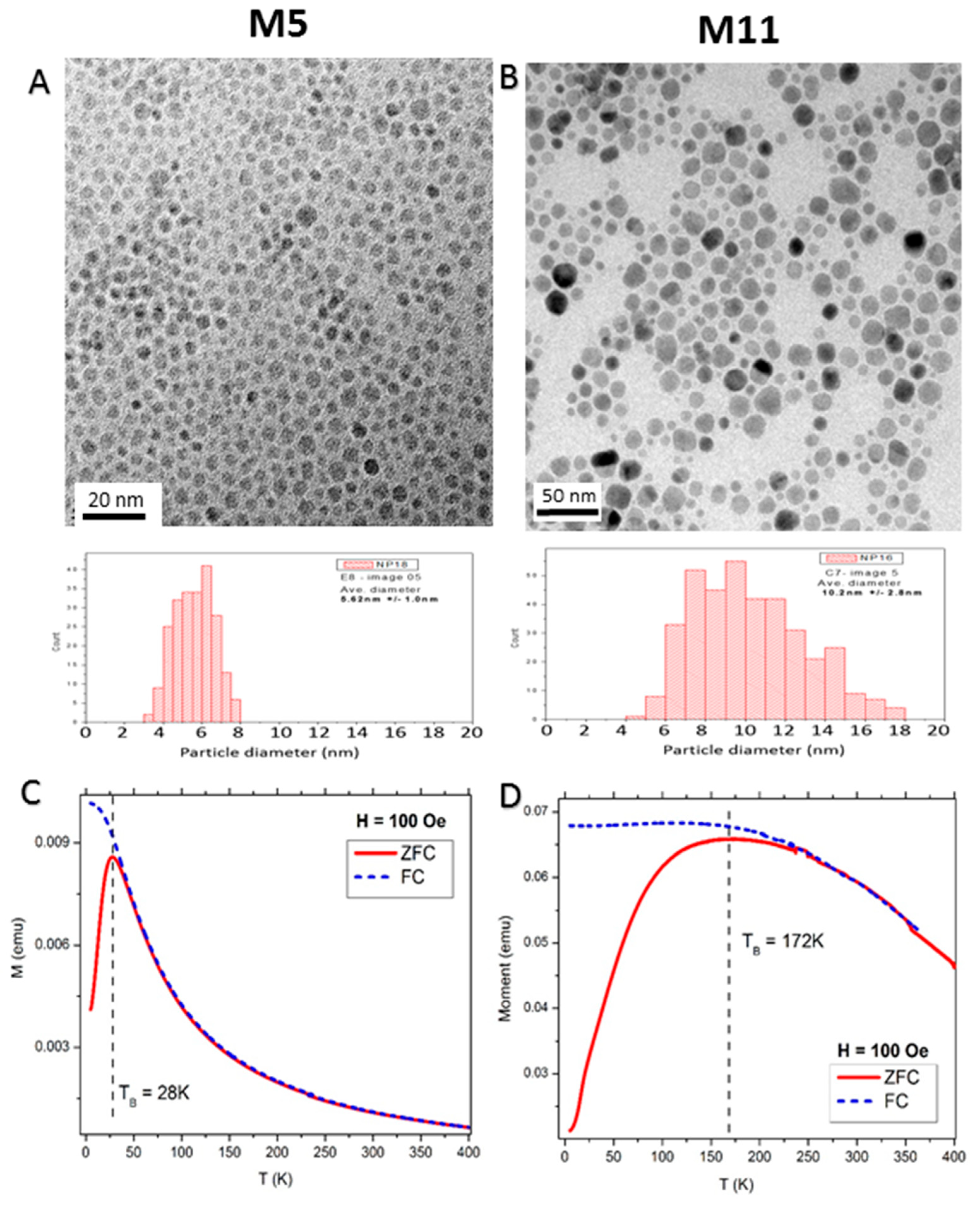
Abstract
:1. Introduction
2. Results
2.1. Structural Properties of the Nanoparticle Assemblies
2.2. Macroscopic Magnetic Properties
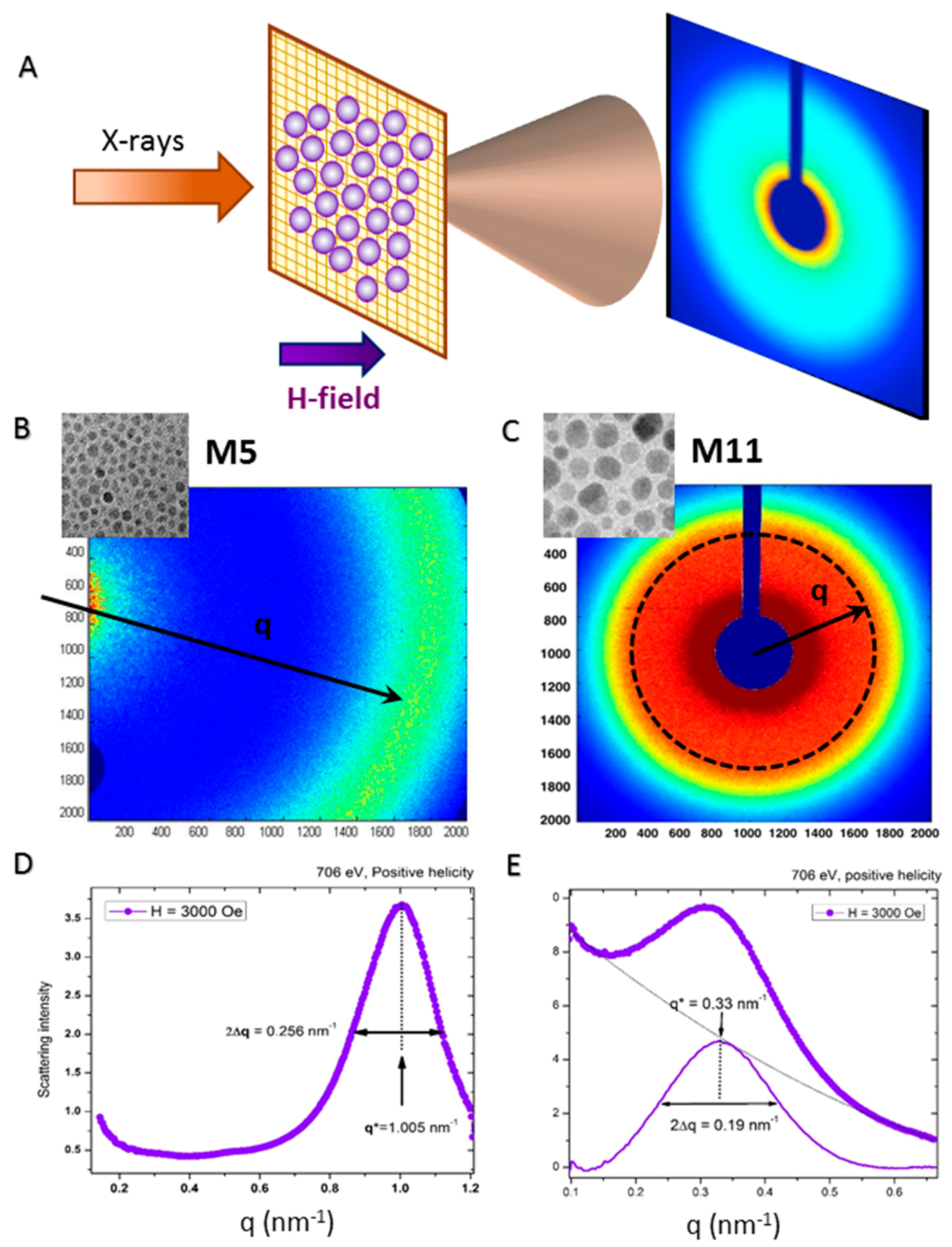
2.3. X-ray Scattering Patterns: Nanoscale Charge Correlations
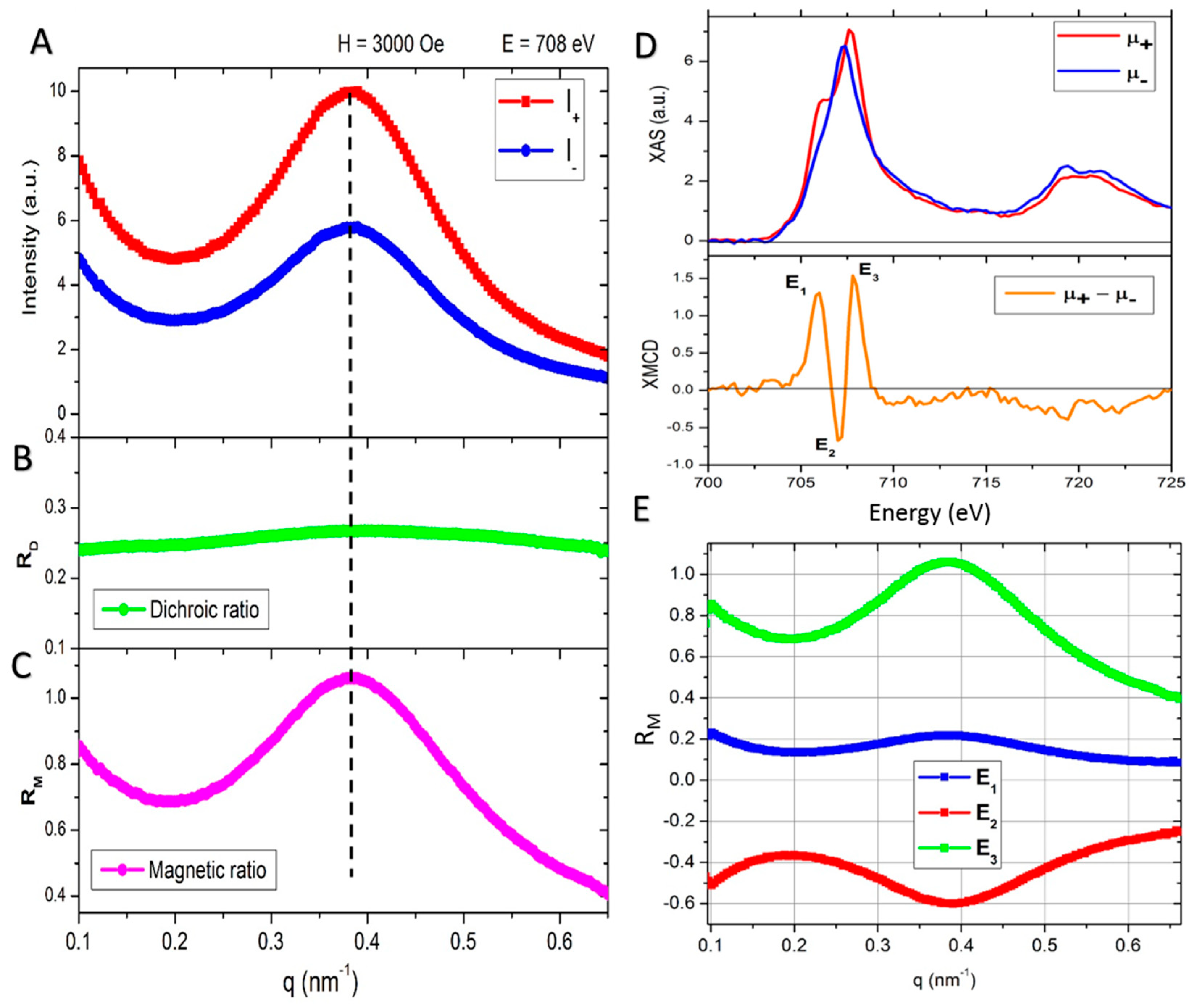
2.4. Extracted Magnetic Scattering: Nanoscale Magnetic Correlations
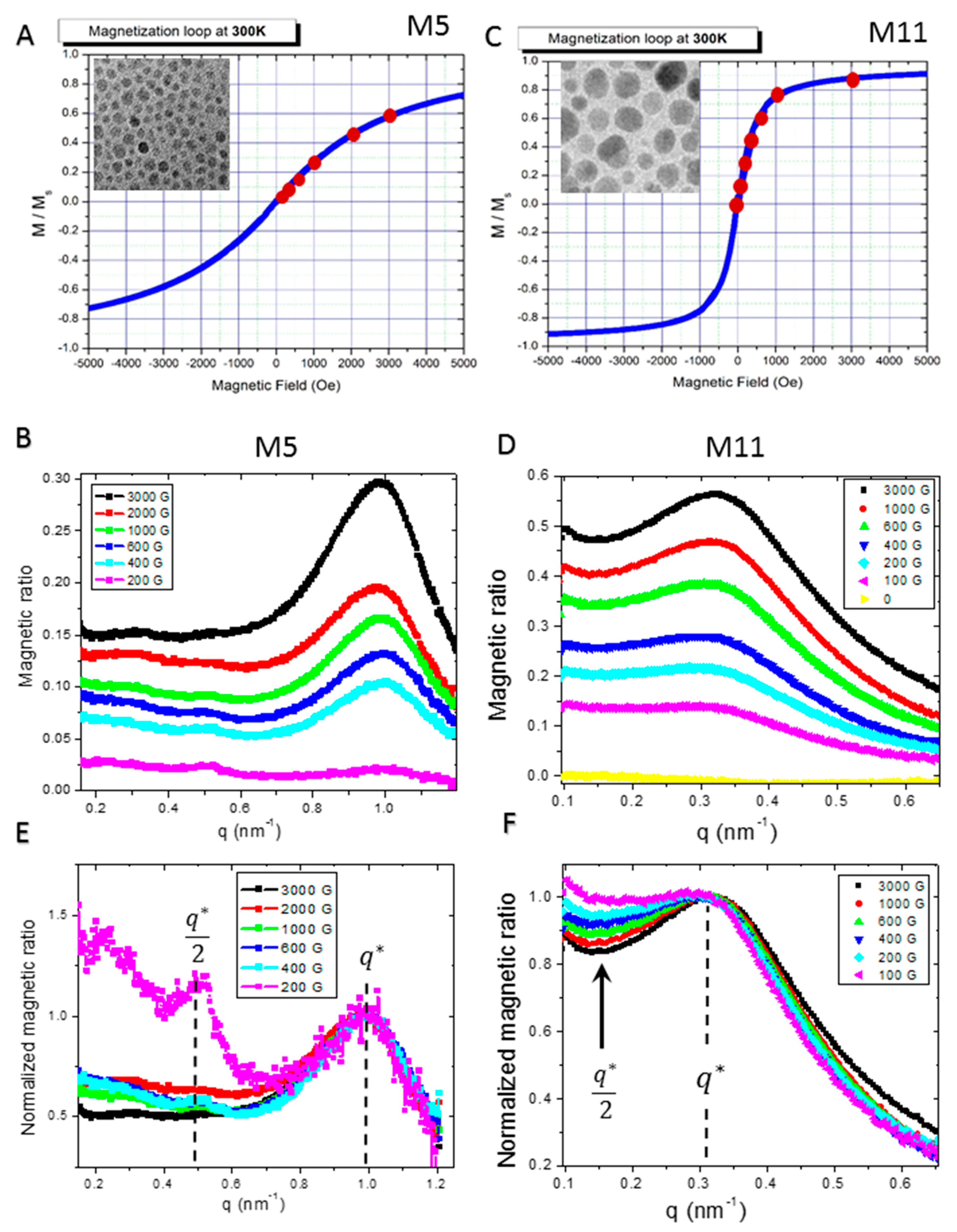
2.5. Dependence on External Magnetic Field
3. Discussion
4. Materials and Methods
5. Conclusions
Author Contributions
Funding
Acknowledgments
Conflicts of Interest
Appendix A
References
- Frey, N.A.; Peng, S.; Cheng, K.; Sun, S. Magnetic nanoparticles: Synthesis, functionalization, and applications in bioimaging and magnetic energy storage. Chem. Soc. Rev. 2009, 38, 2532–2542. [Google Scholar] [CrossRef] [PubMed]
- De, M.; Ghosh, P.S.; Rotello, V.M. Applications of nanoparticles in biology. Adv. Mater. 2008, 20, 4225–4241. [Google Scholar] [CrossRef]
- Majetich, S.A.; Wen, T.; Booth, S.A. Functional magnetic nanoparticle assemblies: Formation, collective behavior and future directions. ACS Nano. 2011, 5, 6081–6084. [Google Scholar] [CrossRef] [PubMed]
- Frey, N.A.; Sun, S. Inorganic Materials; CRC Press: Boca Raton, FL, USA, 2010; pp. 33–68. [Google Scholar]
- Pankhurst, Q.A.; Connolly, J.; Jones, S.K.; Dobson, J. Applications of magnetic nanoparticles in biomedicine. J. Phys. D Appl. Phys. 2003, 36, R167–R181. [Google Scholar] [CrossRef]
- Pankhurst, Q.A.; Thanh, N.T.K.; Jones, S.K.; Dobson, J. Progress in applications of magnetic nanoparticles in biomedicine. J. Phys. D Appl. Phys. 2009, 42, 224001. [Google Scholar] [CrossRef]
- Jun, Y.-W.; Lee, J.H.; Cheon, J. Chemical design of nanoparticle probes for high-performance magnetic resonance imaging. Angew. Chem. Int. Ed. 2008, 47, 5122–5135. [Google Scholar] [CrossRef] [PubMed]
- Berry, C.C.; Curtis, A.S.G. Functionalisation of magnetic nanoparticles for applications in biomedicine. J. Phys. D Appl. Phys. 2003, 36, R198–R208. [Google Scholar] [CrossRef]
- Hergt, R.; Dutz, S.; Muller, R.; Zeisberger, M. Magnetic particle hyperthermia: Nanoparticle magnetism and materials development for cancer therapy. J. Phys. Condens. Matter 2006, 18, S2919–S2934. [Google Scholar] [CrossRef]
- Hanzlik, M.; Heunemann, C.; Holtkamp-Rötzler, E.; Winklhofer, M.; Petersen, N.; Fleissner, G. Superparamagnetic magnetite in the upper beak tissue of homing pigeons. Biometals 2000, 13, 325–331. [Google Scholar] [CrossRef] [PubMed]
- Markides, H.; Rotherham, M.; El Haj, A.J. Biocompatibility and toxicity of magnetic nanoparticles in regenerative medicine. J. Nanomater 2012, 2012, 614094. [Google Scholar] [CrossRef]
- Singh, R.K.; Kim, T.-H.; Patel, K.D.; Knowles, J.; Kim, H.-W. Biocompatible magnetite nanoparticles with varying silica-coating layer for use in biomedicine: Physicochemical and magnetic properties, and cellular compatibility. J. Biomed. Mater. Res. 2012, 100A, 1735. [Google Scholar] [CrossRef] [PubMed]
- Fleet, M.E. The structure of magnetite. Acta Cryst. 1981, B37, 917–920. [Google Scholar] [CrossRef]
- Doriguetto, A.C.; Fernandes, N.G.; Persiano, A.I.C.; Nunes Filho, E.; Grenèche, J.M.; Fabris, J.D. Characterization of a natural magnetite. Phys. Chem. Miner. 2003, 30, 249–255. [Google Scholar]
- Sun, S.; Zeng, H.; Robinson, D.B.; Raoux, S.; Rice, P.M.; Wang, S.X.; Li, G. Monodisperse MFe2O4 (M = Fe, Co, Mn) nanoparticles. J. Am. Chem. Soc. 2004, 126, 273–279. [Google Scholar] [CrossRef] [PubMed]
- Ortega, D.; Vélez-Fort, E.; García, D.A.; García, R.; Litrán, R.; Barrera-Solano, C.; Ramírez-del-Solar, M.; Domínguez, M. Size and surface effects in the magnetic properties of maghemite and magnetite coated nanoparticles. Phil. Trans. R. Soc. A 2010, 368, 4407–4418. [Google Scholar] [CrossRef] [PubMed] [Green Version]
- Cai, Y.; Chesnel, K.; Trevino, M.; Westover, A.; Harrison, R.G.; Hancock, J.M.; Turley, S.; Scherz, A.; Reid, A.; Wu, B.; et al. Orbital and spin moments of 5 to 11 nm Fe3O4 nanoparticles measured via X-ray magnetic circular dichroism. J. Appl. Phys. 2014, 115, 17B537. [Google Scholar] [CrossRef]
- Roca, A.G.; Morales, M.P.; O’Grady, K.; Serna, C.J. Structural and magnetic properties of uniform magnetite nanoparticles prepared by high temperature decomposition of organic precursors. Nanotechnology 2006, 17, 2783–2788. [Google Scholar] [CrossRef]
- Bizdoaca, A.L.; Spasova, M.; Farle, M. Self-assembly and magnetism in core-shell microspheres. J. Vac. Sci. Technol. A 2003, 21, 1515. [Google Scholar] [CrossRef]
- Kralj, S.; Makovec, D. Magnetic assembly of superparamagnetic iron oxide nanoparticle clusters into nanochains and nanobundles. ACS Nano 2015, 9, 0700–9707. [Google Scholar] [CrossRef] [PubMed]
- Goya, G.F.; Berquo, T.S.; Fonseca, F.C.; Morales, M.P. Static and dynamic magnetic properties of spherical magnetite nanoparticles. J. Appl. Phys. 2003, 94, 3520. [Google Scholar] [CrossRef]
- Chesnel, K.; Trevino, M.; Cai, Y.; Hancock, J.M.; Smith, S.J.; Harrison, R.G. Particle size effects on the magnetic behaviour of 5 to 11 nm Fe3O4 nanoparticles coated with oleic acid. J. Phys. Conf. Ser. 2014, 521, 012004. [Google Scholar] [CrossRef]
- Lima, E.; Brand, A.L., Jr.; Arelaro, A.D.; Goya, G.F. Spin disorder and magnetic anisotropy in Fe3O4 nanoparticles. J. Appl. Phys. 2006, 99, 083908. [Google Scholar] [CrossRef]
- Salado, J.; Insausti, M.; Lezama, L.; Gil de Muro, I.; Goikolea, E.; Rojo, T. Preparation and characterization of monodisperse Fe3O4 nanoparticles: An electron magnetic resonance study. Chem. Mater. 2011, 23, 2879–2885. [Google Scholar] [CrossRef]
- Yang, T.; Shen, C.; Li, Z.; Zhang, H.; Xiao, C.; Chen, S.; Xu, Z.; Shi, D.; Li, J.; Gao, H. Highly ordered self-assembly with large area of Fe3O4 nanoparticles and the magnetic properties. J. Phys Chem. B 2005, 109, 23233–23236. [Google Scholar] [CrossRef] [PubMed]
- Varon, M.; Beleggia, M.; Kasama, T.; Harrison, R.J.; Dunin-Borkowski, R.E.; Puntes, V.F.; Frandsen, C. Dipolar magnetism in ordered and disordered low-dimensional nanoparticle assemblies. Sci. Rep. 2013, 3, 1–5. [Google Scholar] [CrossRef] [PubMed] [Green Version]
- Yamamoto, K.; Hogg, C.R.; Yamamuro, S.; Hirayama, T.; Majetich, S. Dipolar ferromagnetic phase transition in Fe3O4 nanoparticle arrays observed by Lorentz microscopy and electron holography. Appl. Phys. Lett. 2011, 98, 072509. [Google Scholar] [CrossRef]
- Campanini, M.; Ciprian, R.; Bedogni, E.; Mega, A.; Chiesi, V.; Casoli, F.; de Julian Fernandez, C.; Rotunno, E.; Rossi, F.; Secchi, A.; et al. Lorentz microscopy sheds light on the role of dipolar interactions in magnetic hyperthermia. Nanoscale 2015, 7, 7717–7735. [Google Scholar] [CrossRef] [PubMed]
- Bellouard, C.; Mirebeau, I.; Hennion, M. Field study of nanoparticles by small angle neutron scattering. J. Magn. Mag. Mater. 1995, 140–144, 431–432. [Google Scholar] [CrossRef]
- Bellouard, C.; Mirebeau, I.; Hennion, M. Magnetic correlations of fine ferromagnetic particles studied by small angle neutron scattering. Phys. Rev. B 1996, 53, 5570. [Google Scholar] [CrossRef]
- Farrell, D.F.; Ijiri, Y.; Kelly, C.V.; Borchers, J.A.; Rhyne, J.J.; Ding, Y.; Majetich, S.A. Small angle neutron scattering study of disordered and crystalline iron nanoparticle assemblies. J. Magn. Mag. Mater. 2006, 303, 318–322. [Google Scholar] [CrossRef]
- Theis-Bröhl, K.; Vreeland, E.C.; Gomez, A.; Huber, D.L.; Saini, A.; Wolff, M.; Maranville, B.B.; Brok, E.; Krycka, K.L.; Dura, J.A.; et al. Self-assembled layering of magnetic nanoparticles in a ferrofluid on silicon surfaces. Appl. Mater. Interfaces 2018, 10, 5050–5060. [Google Scholar] [CrossRef] [PubMed]
- Mishra, D.; Petracic, O.; Devishvili, A.; Theis-Bröhl, K.; Toperverg, B.P.; Zabel, H. Polarized neutron refelectivity from monolayers of self-assembled magnetic nanoparticles. J. Phys.: Condens. Matter 2015, 27, 136001. [Google Scholar]
- Kortright, J.B.; Hellwig, O.; Chesnel, K.; Sun, S.; Fullerton, E.E. Interparticle magnetic correlations in dense Co nanoparticle assemblies. Phys. Rev. B 2005, 71, 012402. [Google Scholar] [CrossRef] [Green Version]
- De Bergevin, F.; Brunel, M. Diffraction of X-rays by magnetic materials. I. General formulae and measurements on ferro- and ferrimagnetic compounds. Acta. Cryst. A 1981, 37, 314–324. [Google Scholar] [CrossRef] [Green Version]
- Hannon, J.P.; Trammell, G.T.; Blume, M.; Gibbs, D. X-ray resonance exchange scattering. Phys. Rev. Lett. 1988, 61, 1245–1248. [Google Scholar] [CrossRef] [PubMed]
- Chesnel, K.; Belakhovsky, M.; Livet, F.; Collins, S.P.; van der Laan, G.; Dhesi, S.S.; Attané, J.P.; Marty, A. Soft-X-ray magnetic speckles from a nanostructured FePd wire. Phys. Rev. B 2002, 66, 172404. [Google Scholar] [CrossRef]
- Chesnel, K.; Turner, J.J.; Pfeifer, M.; Kevan, S.D. Probing complex materials with coherent soft X-rays. Appl. Phys. A Mater. Sci. Process. 2008, 92, 431–437. [Google Scholar] [CrossRef]
- Blume, M. Magnetic scattering of X-rays. J. Appl. Phys. 1985, 57, 3615. [Google Scholar] [CrossRef]
- Hill, J.P.; Mc Morrow, D.F. Resonant exchange scattering: Polarization dependence and correlation function. Acta. Cryst. A 1996, 52, 236. [Google Scholar] [CrossRef]
- Kortright, J.B.; Kim, S.-K.; Denbeaux, G.P.; Zeltzer, G.; Takano, K.; Fullerton, E.E. Soft-X-ray small-angle scattering as a sensitive probe of magnetic and charge heterogeneity. Phys. Rev. B 2001, 64, 092401. [Google Scholar] [CrossRef]
- Huang, D.J.; Chang, C.F.; Jeng, H.-T.; Guo, G.Y.; Lin, H.-J.; Wu, W.B.; Ku, H.C.; Fujimori, A.; Takahashi, Y.; Chen, C.T. Spin and orbital magnetic moments of Fe3O4. Phys. Rev. Lett. 2004, 93, 077204. [Google Scholar] [CrossRef] [PubMed]
- Gomes, G.F.M.; Bueno, T.E.P.; Parreiras, D.E.; Abreu, G.J.P.; de Siervo, A.; Cezar, J.C.; Pfannes, H.-D.; Paniago, R. Magnetic moment of Fe3O4 films with thicknesses near the unit-cell size. Phys. Rev. B 2014, 90, 134422. [Google Scholar] [CrossRef]
- Fjellvåg, H.; Grønvold, F.; Stølen, S. On the crystallographic and magnetic structures of nearly stoichiometric iron monoxide. J. Solid State Chem. 1996, 124, 52–57. [Google Scholar] [CrossRef]
- Hansen, M.F.; Morup, S. Models for the dynamics of interacting magnetic nanoparticles. J. Magn. Mag. Mater. 1998, 184, 262–274. [Google Scholar] [CrossRef]
- Lee, H.K. Monte Carlo simulations of interacting magnetic nanoparticles. J. Appl. Phys. 2002, 91, 6926. [Google Scholar] [CrossRef]
- Altavilla, C.; Ciliberto, E.; Gatteschi, D.; Sangregorio, C. A new route to fabricate monolayers of magnetite nanoparticles on silicon. Adv. Mater. 2005, 17, 1084. [Google Scholar] [CrossRef]
- Guardia, P.; Perez, N.; Labarta, A.; Battle, X. Controlled synthesis of iron oxide nanoparticles over a wide size range. Langmuir 2010, 26, 5843–5847. [Google Scholar] [CrossRef] [PubMed]
- Turner, J.J.; Thomas, K.J.; Hill, J.P.; Pfeifer, M.A.; Chesnel, K.; Tomioka, Y.; Tokura, Y.; Kevan, S.D. Orbital domain dynamics in a doped manganite. New. J. Phys. 2008, 10, 053023. [Google Scholar] [CrossRef] [Green Version]
- Chesnel, K.; Safsten, A.; Rytting, M.; Fullerton, E. Shaping nanoscale magnetic domain memory in exchange-coupled ferromagnets by field cooling. Nat. Commun. 2016, 7, 11648. [Google Scholar] [CrossRef] [PubMed] [Green Version]
- Tripathi, A.; Mohanty, J.; Dietze, S.H.; Shpyrko, O.G.; Shipton, E.; Fullerton, E.E.; Kim, S.S.; McNulty, I. Dichroic coherent diffractive imaging. PNAS 2011, 108, 13393–13398. [Google Scholar] [CrossRef] [PubMed]
- Kortright, J.B.; Rice, M.; Carr, R. Soft-X-ray Faraday rotation at Fe L2,3 edges. Phys. Rev. B 1995, 51, 10240. [Google Scholar] [CrossRef]

© 2018 by the authors. Licensee MDPI, Basel, Switzerland. This article is an open access article distributed under the terms and conditions of the Creative Commons Attribution (CC BY) license (http://creativecommons.org/licenses/by/4.0/).
Share and Cite
Chesnel, K.; Griner, D.; Smith, D.; Cai, Y.; Trevino, M.; Newbold, B.; Wang, T.; Liu, T.; Jal, E.; Reid, A.H.; et al. Unraveling Nanoscale Magnetic Ordering in Fe3O4 Nanoparticle Assemblies via X-rays. Magnetochemistry 2018, 4, 42. https://doi.org/10.3390/magnetochemistry4040042
Chesnel K, Griner D, Smith D, Cai Y, Trevino M, Newbold B, Wang T, Liu T, Jal E, Reid AH, et al. Unraveling Nanoscale Magnetic Ordering in Fe3O4 Nanoparticle Assemblies via X-rays. Magnetochemistry. 2018; 4(4):42. https://doi.org/10.3390/magnetochemistry4040042
Chicago/Turabian StyleChesnel, Karine, Dalton Griner, Dallin Smith, Yanping Cai, Matea Trevino, Brittni Newbold, Tianhan Wang, Tianmin Liu, Emmanuelle Jal, Alex H. Reid, and et al. 2018. "Unraveling Nanoscale Magnetic Ordering in Fe3O4 Nanoparticle Assemblies via X-rays" Magnetochemistry 4, no. 4: 42. https://doi.org/10.3390/magnetochemistry4040042
APA StyleChesnel, K., Griner, D., Smith, D., Cai, Y., Trevino, M., Newbold, B., Wang, T., Liu, T., Jal, E., Reid, A. H., & Harrison, R. G. (2018). Unraveling Nanoscale Magnetic Ordering in Fe3O4 Nanoparticle Assemblies via X-rays. Magnetochemistry, 4(4), 42. https://doi.org/10.3390/magnetochemistry4040042