Artificial Neural Network-Based Heat Transfer Analysis of Sutterby Magnetohydrodynamic Nanofluid with Microorganism Effects

Abstract

Background: The study of non-Newtonian fluids in thin channels is crucial for advancing technologies in microfluidic systems and targeted industrial coating processes. Nanofluids, which exhibit enhanced thermal properties, are of particular interest. This paper investigates the complex flow and heat transfer characteristics of a Sutterby nanofluid (SNF) within a thin channel, considering the combined effects of magnetohydrodynamics (MHD), Brownian motion, and bioconvection of microorganisms. Analyzing such systems is essential for optimizing design and performance in relevant engineering applications. Method: The governing non-linear partial differential equations (PDEs) for the flow, heat, concentration, and bioconvection are derived. Using lubrication theory and appropriate dimensionless variables, this system of PDEs is simplified into a more simplified system of ordinary differential equations (ODEs). The resulting nonlinear ODEs are solved numerically using the boundary value problem (BVP) Midrich method in Maple software to ensure accuracy. Furthermore, data for the Nusselt number, extracted from the numerical solutions, are used to train an artificial neural network (ANN) model based on the Levenberg–Marquardt algorithm. The performance and predictive capability of this ANN model are rigorously evaluated to confirm its robustness for capturing the system’s non-linear behavior. Results: The numerical solutions are analyzed to understand the variations in velocity, temperature, concentration, and microorganism profiles under the influence of various physical parameters. The results demonstrate that the non-Newtonian rheology of the Sutterby nanofluid is significantly influenced by Brownian motion, thermophoresis, bioconvection parameters, and magnetic field effects. The developed ANN model demonstrates strong predictive capability for the Nusselt number, validating its use for this complex system. These findings provide valuable insights for the design and optimization of microfluidic devices and specialized coating applications in industrial engineering.

1. Introduction

Deep neural networks (DNNs), a specialized class of ANNs, consist of multiple hidden layers that enable them to capture and represent highly complex nonlinear relationships between inputs and outputs. Their hierarchical depth allows for the automatic extraction of high-level features from raw data, making them exceptionally effective in modeling sophisticated physical processes [1,2,3]. In the field of fluid mechanics, DNNs are particularly valuable as they can approximate intricate flow dynamics, capture turbulence effects, and incorporate both experimental and simulated datasets into predictive frameworks. This reduces the reliance on costly and time-consuming laboratory experiments. When coupled with the Levenberg–Marquardt backpropagation algorithm, an optimization scheme for nonlinear least squares problems, DNNs exhibit enhanced stability and faster convergence during training. The LM method is extensively utilized in fluid mechanics to align experimental or numerical data with mathematical models by minimizing the squared error between the measured results and the predicted values. Backpropagation, originally introduced by Werbos in 1974, uses gradient descent to minimize network error, while the LM algorithm ensures improved convergence and robustness of ANNs in addressing fluid dynamics problems. Several studies highlight the integration of these techniques in practical applications. Kutz [3] applied an ANN trained with the LMB algorithm to investigate heat transfer in nanofluid flows between parallel plates, accounting for Brownian motion and thermophoretic effects. Abbas [4] developed a wire-coating model with ANNs-LMA to replicate the behavior of Eyring–Powell fluids under various conditions. Elshehabey [5] integrated ANNs with the finite element method to investigate entropy generation and heat transfer in MHD natural convection of nanofluids inside an inclined cavity with an H-shaped obstacle. Hira et al. [6] predicted the flow of MWCNT-Al₂O₃/SAE 40 nano-lubricant using ANN models, while Mandal et al. [7] investigated the influence of non-Darcian porous media in M-shaped cavities. Beyond fluid mechanics, ANNs have also been applied in areas such as solid waste management [8] and even explored in the context of quantum computing [9], further demonstrating their versatility across scientific and engineering domains [10,11,12].

While machine learning frameworks such as DNNs offer powerful predictive capabilities in fluid mechanics, an accurate representation of flow dynamics still requires reliable constitutive fluid models. In this regard, nanofluids and non-Newtonian fluids have attracted growing attention due to their enhanced transport properties and complex rheology. Recently, attention has turned to hybrid nanofluids, which incorporate multiple nanoparticles suspended in base fluids (see Figure 1). These advanced fluids show promise for diverse mass and heat transfer applications in microfluidics, fabrication, energy transport, and defense industries [13,14]. Moreover, in contrast to Newtonian fluids, non-Newtonian fluids play a fundamental role in several industrial and biological processes, including emulsions, paper manufacturing, nuclear fuel slurries, polymer lubricants, food processing, biomedical fluids, and tissue mechanics [15]. Their complex rheological behavior is captured by various models such as Carreau, Jeffery, Sisko, Williamson, Power-law, and Sutterby nanofluid models, each designed to represent specific fluid characteristics [16,17,18,19,20]. Among these, the Sutterby nanofluid model has received comparatively less attention in the literature, despite its strong potential for industrial and engineering applications.

The Sutterby model, first presented in 1966, is widely recognized for its effectiveness in describing the complex rheology of polymer melts and solutions. As a notable non-Newtonian formulation, it accounts for both shear-thinning and shear-thickening behaviors, making it suitable for modeling realistic fluid responses in engineering, biomedical, and industrial applications, especially in boundary layer flows. Over the years, many studies have analyzed Sutterby fluids under numerous conditions, together with natural, forced convection, and mixed, as well as cases involving uniform or non-uniform heating and the inclusion of nanoparticles. Because the governing equations are highly nonlinear and complicated, different computational and semi-analytical approaches have been applied to study their behavior. These approaches include the Homotopy Analysis Method (HAM), perturbation methods, the Runge–Kutta–Fehlberg (RKF) technique, and discretization-based numerical methodologies like finite difference and finite element methods [21]. Collectively, these studies highlight the Sutterby model’s capability to capture complex non-linear flow dynamics across a wide spectrum of industrial and biological systems [22].

An additional dimension of complexity arises from MHD, which combines electromagnetism and fluid dynamics to study electrically conducting fluids under magnetic fields. Owing to its broad applicability, MHD has been extensively employed in engineering systems and astrophysical phenomena. Raju et al. [23] explored the unsteady MHD flow of a thermally responsive fluid over a moving plate, incorporating the effects of porosity, buoyancy, and plate inclination. Devi et al. [24] deliberated the boost in the rate of transfer rate by via the hybrid nanofluid in a three-dimensional stretchable surface with Newton heating and MHD effects. Jaluria and Gebhart [25] investigated the stability and transition behavior of buoyancy-driven flows in stratified fluids, emphasizing the role of thermal gradients. Their research further examined the impact of internal heat generation on the bioconvective dynamics of MHD nanofluid flows containing gyrotactic microorganisms. Similarly, Rubab et al. [26] reported on energy absorption in tangent hyperbolic MHD flows. These studies collectively highlight the importance of MHD in enhancing heat and mass transfer, but also demonstrate the challenges of modeling nonlinear coupled effects.

Bioconvection refers to the large-scale fluid motion generated by the collective swimming of motile microorganisms, such as algae or bacteria, which are typically denser than the surrounding medium. Their upward movement creates unstable density stratification that gives rise to convective plumes and mixing patterns within the fluid. Bioconvection induced by motile microorganisms enhances mixing and alters heat and mass transfer in nanofluids. In coating processes, this can lead to more uniform deposition and improved coating quality. Microorganisms increase effective viscosity and modify flow structures, which influence coating thickness and stability.

This phenomenon was first described by Platt [27] in relation to suspensions of free-swimming organisms and later examined in detail through continuum models, such as those developed by Pedley et al. [28] for gyrotactic microorganisms. Bioconvection not only enhances mixing and alters mass and heat transfer in nanofluid systems but also plays a vital role in natural environments, where it contributes to nutrient cycling, phytoplankton blooms, and ecosystem stability. Beyond ecology, it has gained growing attention in biomedical and industrial fluid mechanics due to its potential impact on microfluidic processes, coating technologies, and transport phenomena involving complex fluids. Numerous studies have explored the phenomenon of bioconvection in different fluid flow configurations. For instance, Kamal et al. [29] examined Marangoni convection with gyrotactic microorganisms in Maxwell fluids over a rotating disk and analyzed entropy generation to assess system reversibility. Nayak et al. [30] investigated chemically reactive bioconvective nanofluid flow past an exponentially stretching sheet with motile microorganisms, employing Buongiorno’s model to account for Brownian motion and thermophoretic diffusion. Ahmad et al. [31] studied nanofluid transport through porous media and highlighted the role of gyrotactic microbes in altering flow characteristics. More recently, Galal M. Moatimid et al. [32] analyzed the bioconvective behavior of Sutterby nanofluids containing microorganisms over a stretched sheet with variable viscosity, showing that viscosity variations promote microbial growth, whereas larger Lewis Peclet numbers suppress it, thereby modifying mass and heat transfer mechanisms. Interest in non-Newtonian nanofluids has continued to grow due to their enhanced thermal and rheological properties. These findings reinforce the potential of bioconvection studies in coating technologies and microfluidic systems [33,34].

Among numerous industrial applications, reverse roll coating (RRC) is regarded as a highly common coating method, favored for its affordability and ease of operation. It works by introducing the coating fluid into the gap created between two rollers rotating in opposite directions. Greener and Middleman [35] examined the RRC process of a viscoelastic fluid utilizing the conventional LAT and derived the solution through the perturbation approach. They noted a decline in pressure with a slight increase in coating thickness. In earlier studies, Coyle [36] conducted a thorough examination of the fluid dynamics of RC, focusing on steady flows, rheology, and stability, and clarifying the essential flow characteristics, stability factors, and rheological influences involved in these processes. Hinter and White et al. [37] investigated the water flow that occurs between two rolls in their research results. Using the lubrication principle, the results were verified to match the experimental findings. In their analysis of RRC systems, Greener and Middleman et al. [35] used mathematical models rooted in lubrication theory. However, these models omitted to take surface tension, free surfaces, and contact line behaviour into consideration. Benkreira et al. [38] implemented analytic and computational methodologies to examine the flow characteristics of coatings for a variety of fluid types, including Newtonian and non-Newtonian fluids. Early numerical investigations by Ascanio et al. [39] focused on high-speed RC using fluids with complex rheology, establishing foundational methodologies for simulating viscous flows. In order to explore the importance of fluid properties in the RRC process, Jang and Chen [40] developed this research by taking into account the volume of fluid-free surface and finite-volume methodologies. The RC process was analyzed using the non-Newtonian power-law fluid model, with the power-law index varying between 0.95 and 1.05. Additionally, Shahzad et al. [41] investigated the behavior of a non-isothermal couple stress fluid within an RRC configuration, taking into account the slip conditions present at the surfaces of the rolls. Devisetti et al. [42] further explored fluid absorption effects in forward roll coating (FRC), emphasizing the role of rheological properties in optimizing industrial efficiency, particularly for non-Newtonian lubricants. These studies confirm that fluid rheology strongly influences coating uniformity and efficiency, making RRC an ideal context to examine the behavior of non-Newtonian nanofluids. Further studies on the application of ANN for fluids and nanofluids can be found in the references [43,44,45,46,47].

1.1. Motivation for the Work

Motivated by the above-cited literature, which highlights both the potential and the limitations of existing analytical and numerical methods, the present study develops a hybrid numerical-neural approach. The velocity, temperature, concentration, microorganism distribution, and skin friction profiles are obtained through the Midrich BVP numerical method, while an ANN with three hidden layers, trained using the LMB algorithm and the sigmoid activation function, is applied to achieve high-accuracy predictions of the Nusselt number in a thin channel formed by two rolls rotating in opposite directions. This integrated framework provides a robust and efficient alternative to conventional approaches, supporting improved process optimization, enhanced coating quality, and reduced material waste. Furthermore, the study addresses the gap between theoretical modeling and industrial coating requirements, contributing to improved efficiency and sustainability in manufacturing operations. The main contributions of this work are as follows:

• To capture the rheological behavior of fluids with suspended nanoparticles and gyrotactic microorganisms, the non-Newtonian Sutterby fluid model is applied.
• This research provides a comprehensive investigation of material parameters such as the velocity ratio, MHD, Brownian motion, and others on their influence on the behavior of Sutterby nanofluid in the context of the RRC process.
• Moreover, the LM technique is employed to analyze heat transfer, and the results of the LMB-NNs are compared with the Midrich BVP numerical solutions of the SNFM.
• The mean squared error (MSE) index is computed, and various statistical analyses are performed to evaluate the accuracy of the proposed model.
• Furthermore, an ANN with three hidden layers, trained using the LMB algorithm and the log-sigmoid activation function, is applied to achieve high-accuracy predictions.

1.2. Research Gap

Despite extensive investigations into non-Newtonian fluids, the intricate interplay of Sutterby rheology, magnetohydrodynamics, and bioconvection in the context of reverse roll coating (RRC) remains scarcely investigated. Furthermore, while numerical methods and machine learning have advanced independently, a hybrid framework that seamlessly integrates high-fidelity numerical solutions with artificial intelligence for predictive modeling in such complex flows is notably absent from the literature. This work bridges this critical gap by introducing a novel methodology that couples the BVP–Midrich numerical solver with an ANN-LMA to accurately analyze and predict the thermal and hydrodynamic behavior of a Sutterby nanofluid containing motile microorganisms. This integrated approach not only elucidates the underlying physics but also establishes a robust, efficient computational paradigm for optimizing industrial coating processes, thereby paving the way for enhanced product quality and operational sustainability.

1.3. Structure of the Paper

The manuscript is organized into several sections, and their details are schematically illustrated in the flow chart presented in Figure 2.

The present work contributes to the existing literature by addressing the following critical questions:

i.

How does the nanoparticle volume fraction affect the flow behavior and thermal characteristics of the current flow system?

ii.

In what ways do the velocity ratio, Schmidt number, and Brownian motion parameter influence the fluid velocity, temperature, concentration, and microorganism distribution?

iii.

How can various parameters influence the heat transfer characteristics, as analyzed through the ANNs-LMA framework?

iv.

What is the combined impact of these fluid parameters on heat transfer, and how can this influence be effectively summarized in tabular form?

2. Problem Statement and Mathematical Modeling

2.1. Assumptions of the Present Fluid Model

• The flow is two-dimensional, steady, and laminar.
• The fluid is incompressible.
• The fluid is modeled as a non-Newtonian Sutterby MHD nanofluid.
• The flow occurs between two infinitely long rolls rotating in opposite directions with angular velocities $U_f=R{\omega }_f$ (forward roll) and $U_r=R{\omega }_r$ (reverse roll), where $R$ stand for the radius of each roll and subscript $f$ and $r$ stand for forward and reverse rotating.
• The gap between the rolls is $2H_0$.
• The velocity ratio $k={\displaystyle \frac{U_r}{U_f}}$ is uniform across the rolls.
• The flow is driven by the rotation of the rolls; no external pressure gradient is applied.
• The coordinate system is defined such that the $x-axis$ is aligned along the flow direction between the rolls and the $y-axis$ is perpendicular to it (transversal). Figure 3 illustrates the geometry of the physical model considered in the present investigation.

2.2. Governing Equations

From the preceding assumptions and the constitutive model of the Sutterby nanofluid, the governing equations for steady laminar flow are formulated. These equations, expressed in component form, govern momentum, heat transfer, microorganism distribution, and nanoparticle concentration within the boundary layer, as shown below:

Continuity equation:

$${\displaystyle \frac{\partial \overline{u}}{\partial \overline{x}}}+{\displaystyle \frac{\partial \overline{v}}{\partial \overline{y}}}=0,$$

(1)

Momentum equation:

$${\rho }_f\left(\overline{u}{\displaystyle \frac{\partial \overline{u}}{\partial \overline{x}}}+\overline{v}{\displaystyle \frac{\partial \overline{u}}{\partial \overline{y}}}\right)=-{\displaystyle \frac{\partial \overline{p}}{\partial \overline{x}}}+{\displaystyle \frac{\partial {\overline{\tau }}_{xx}}{\partial \overline{x}}}+{\displaystyle \frac{\partial {\overline{\tau }}_{xy}}{\partial \overline{y}}}-\sigma B_0^2\overline{u}+\left[\begin{array}{l}g{\rho }_f{B}^{\ast }\left(1-C_{\infty }\right)\left(T-T_{\infty }\right)\\ -g\left({\rho }_p-{\rho }_f\right)\left(C-C_{\infty }\right)\\ -g{\gamma }^{\ast }\left({\rho }_m-{\rho }_f\right)\left(N-N_{\infty }\right)\end{array}\right],$$

(2)

Energy Equation:

$$\left\{\begin{array}{l}{\left(\rho c\right)}_{nf}\left(\overline{u}{\displaystyle \frac{\partial T}{\partial \overline{x}}}+\overline{v}{\displaystyle \frac{\partial T}{\partial \overline{y}}}\right)=k\left[{\displaystyle \frac{{\partial }^{2}T}{\partial {\overline{x}}^2}}+{\displaystyle \frac{{\partial }^{2}T}{\partial {\overline{y}}^2}}\right]+{\overline{\tau }}_{xx}{\displaystyle \frac{\partial \overline{u}}{\partial \overline{x}}}+{\overline{\tau }}_{xy}\left({\displaystyle \frac{\partial \overline{u}}{\partial \overline{y}}}+{\displaystyle \frac{\partial \overline{v}}{\partial \overline{x}}}\right)+{\overline{\tau }}_{yy}{\displaystyle \frac{\partial \overline{v}}{\partial \overline{y}}}\\ \hspace{0.33em}\hspace{0.33em}\hspace{0.33em}\hspace{0.33em}\hspace{0.33em}\hspace{0.33em}\hspace{0.33em}\hspace{0.33em}\hspace{0.33em}\hspace{0.33em}\hspace{0.33em}\hspace{0.33em}\hspace{0.33em}+{\left(\rho c\right)}_{np}\left\{\begin{array}{l}{D}_B\left({\displaystyle \frac{\partial T}{\partial \overline{x}}}\cdot {\displaystyle \frac{\partial C}{\partial \overline{x}}}\right)+\left({\displaystyle \frac{\partial T}{\partial \overline{y}}}\cdot {\displaystyle \frac{\partial C}{\partial \overline{y}}}\right)\\ +{\displaystyle \frac{D_T}{T_1}}\left[{\left({\displaystyle \frac{\partial T}{\partial \overline{x}}}\right)}^2+{\left({\displaystyle \frac{\partial T}{\partial \overline{y}}}\right)}^2\right]\end{array}\right\} \hspace{0.33em}-{\displaystyle \frac{\partial q_r}{\partial \overline{y}}}+q_T\left(T-T_{\infty }\right),\hspace{0.33em}\hspace{0.33em} \end{array}\right.$$

(3)

Concentration Equation:

$$\left(\overline{u}{\displaystyle \frac{\partial C}{\partial \overline{x}}}+\overline{v}{\displaystyle \frac{\partial C}{\partial \overline{y}}}\right)=D_B\left[{\displaystyle \frac{{\partial }^{2}C}{\partial {\overline{x}}^2}}+{\displaystyle \frac{{\partial }^{2}C}{\partial {\overline{y}}^2}}\right]+{\displaystyle \frac{D_T}{T_1}}\left[{\displaystyle \frac{{\partial }^{2}T}{\partial {\overline{x}}^2}}+{\displaystyle \frac{{\partial }^{2}T}{\partial {\overline{y}}^2}}\right]-K_r^2\left(C-C_{\infty }\right){\left({\displaystyle \frac{T}{T_{\infty }}}\right)}^n\exp \left({\displaystyle \frac{E_a}{KT}}\right),$$

(4)

Micro-Organisms Equation:

$$\left(\overline{u}{\displaystyle \frac{\partial N}{\partial \overline{x}}}+\overline{v}{\displaystyle \frac{\partial N}{\partial \overline{y}}}\right)=D_m\left[{\displaystyle \frac{{\partial }^{2}N}{\partial {\overline{x}}^2}}+{\displaystyle \frac{{\partial }^{2}N}{\partial {\overline{y}}^2}}\right]-{\displaystyle \frac{\partial T}{\partial \overline{y}}}\left(N{\displaystyle \frac{\partial C}{\partial \overline{y}}}\right){\displaystyle \frac{b{w}_c}{\left(C_w-C_{\infty }\right)}},$$

(5)

Boundary conditions (BCs) [35] are:

$$\left\{\begin{array}{l}\hspace{0.33em}\hspace{0.33em}u=U_f,\hspace{0.33em}\hspace{0.33em}\hspace{0.33em}\hspace{0.33em}T=T_0,\hspace{0.33em}\hspace{0.33em}\hspace{0.33em}\hspace{0.33em}\hspace{0.33em}C=C_1,\hspace{0.33em}\hspace{0.33em}\hspace{0.33em}N=N_1,\hspace{0.33em}\hspace{0.33em}\hspace{0.33em}\hspace{0.33em}\hspace{0.33em}\hspace{0.33em}\mathrm{at}\hspace{0.33em}\hspace{0.33em}\hspace{0.33em}y=h\left(x\right),\\ u=-U_r,\hspace{0.33em}\hspace{0.33em}\hspace{0.33em}T=0,\hspace{0.33em}\hspace{0.33em}\hspace{0.33em}\hspace{0.33em}C=0,\hspace{0.33em}\hspace{0.33em}\hspace{0.33em}\hspace{0.33em}N=0,\hspace{0.33em}\hspace{0.33em}\hspace{0.33em}\hspace{0.33em}\hspace{0.17em}\hspace{0.17em}\hspace{0.17em}\hspace{0.17em}\hspace{0.17em}\hspace{0.17em}\hspace{0.17em}\hspace{0.17em}\hspace{0.17em}\hspace{0.17em}\mathrm{at}\hspace{0.33em}\hspace{0.33em}\hspace{0.33em}y=-h\left(x\right).\end{array}\right.$$

(6)

2.3. Rheological Model

Our primary focus is to analysis the S-N-F-M during the RRC process. The mathematical equations that signify the S-N-F-M can be presented in the following way.

$$S=-\overline{p}I+\overline{\tau }.$$

(7)

The SNFM rheological model equation:

$$\overline{\tau }={\mu }_0{\left[{\displaystyle \frac{{\mathrm{Sinh}}^{-1}\left(B\gamma \right)}{\left(B\gamma \right)}}\right]}^m{A}_1,c$$

(8)

Extra stress tensor of Sutterby Nanofluid:

$${\overline{\tau }}_{yx}={\overline{\tau }}_{xy}={\mu }_0\left[1-{\displaystyle \frac{m{B}^2}{6}}\left\{2\left({\left({\displaystyle \frac{\partial \overline{v}}{\partial \overline{y}}}\right)}^2+{\left({\displaystyle \frac{\partial \overline{u}}{\partial \overline{x}}}\right)}^2\right)+{\left({\displaystyle \frac{\partial \overline{v}}{\partial \overline{x}}}+{\displaystyle \frac{\partial \overline{u}}{\partial \overline{y}}}\right)}^2\right\}\right]2\left({\displaystyle \frac{\partial \overline{u}}{\partial \overline{x}}}+{\displaystyle \frac{\partial \overline{v}}{\partial \overline{y}}}\right),$$

(9)

2.4. The Dimensionless Form

The use of dimensionless parameters is fundamental in fluid mechanics, as they not only simplify the governing equations but also provide deeper insights into the underlying physical mechanisms. These parameters allow generalization across different systems and make it possible to identify the dominant effects in various flow regimes. In this section, the non-dimensional equations for the non-isothermal RRC process are derived and subsequently simplified using the LAT approach. The most significant dynamic events happen in the nip region of the RRC procedure. In that area, enlarging to any side by a small distance, the surface of the roll is almost parallel. Then, it is equitable to take up that $uv$ and ${\displaystyle \frac{\partial }{\partial y}}{\displaystyle \frac{\partial }{\partial x}}$. The material travels in the $x$- direction, and there is no velocity that can be observed in the $y$-direction. The associated dimensionless variables are introduced in accordance with the previously conducted order-of-magnitude analysis [35]:

$$\left.\begin{array}{l}{u}^{\ast }={\displaystyle \frac{\overline{u}}{U}},v^{\ast }={\displaystyle \frac{\overline{v}}{\beta U}},x^{\ast }={\displaystyle \frac{\overline{x}}{{\left(R{H}_0\right)}^{\frac{1}{2}}}},y^{\ast }={\displaystyle \frac{\overline{y}}{H_0}},p^{\ast }={\displaystyle \frac{\overline{p}{H}_0^{\frac{3}{2}}}{\mu U{R}^{\frac{1}{2}}}},{\gamma }^{\ast }={\displaystyle \frac{\gamma H_0}{U}},{\mu }^{\ast }=\overline{\mu }{\mu }_0,\\ \beta =\sqrt{{\displaystyle \frac{H_0}{R}}},{\tau }_{xy}^{\ast }={\displaystyle \frac{{\overline{\tau }}_{xy}{H}_0}{\mu U}},{\tau }_{xx}^{\ast }={\displaystyle \frac{{\overline{\tau }}_{xx}{H}_0}{\mu U}},{\tau }_{yy}^{\ast }={\displaystyle \frac{{\overline{\tau }}_{yy}{H}_0}{\mu U}},h^{\ast }\left(x^{\ast }\right)={\displaystyle \frac{\overline{h\left(x\right)}}{H_0}}=1+x^2,\\ \theta ={\displaystyle \frac{T-T_{\infty }}{T_w-T_{\infty }}},\chi ={\displaystyle \frac{\left(N-N_{\infty }\right)}{\left(N_w-N_{\infty }\right)}},\varphi ={\displaystyle \frac{\left(C-C_{\infty }\right)}{\left(C_w-C_{\infty }\right)}},\end{array}\right\},$$

(10)

making use of Equation (10) into Equations (1)–(6), and after omitting the steric $(\ast )$ for ease, the simplifying dimensionless forms are shown as follows:

$${\displaystyle \frac{\partial u}{\partial x}}+{\displaystyle \frac{\partial v}{\partial y}}=0,$$

(11)

$$\left({\displaystyle \frac{{\partial }^2}{\partial y^2}}u\left(y\right)\right)\left[1-We{\left({\displaystyle \frac{\partial }{\partial y}}u\left(y\right)\right)}^2\right]-M^{2}u\left(y\right)+Gr\left(\theta \left(y\right)-N_r\varphi \left(y\right)-R_b\chi \left(y\right)\right)={\displaystyle \frac{d}{dx}}p\left(x\right).$$

(12)

$$\begin{array}{l}\left(1+{\displaystyle \frac{4}{3Nr}}\right)\left({\displaystyle \frac{{\partial }^2}{\partial y^2}}\theta \left(y\right)\right)+Br\left[1-We{\left({\displaystyle \frac{\partial }{\partial y}}u\left(y\right)\right)}^2\right]\left({\displaystyle \frac{{\partial }^2}{\partial y^2}}u\left(y\right)\right)+Nb\left({\displaystyle \frac{\partial }{\partial y}}\theta \left(y\right)\cdot {\displaystyle \frac{\partial }{\partial y}}\varphi \left(y\right)\right)\\ \hspace{0.33em}\hspace{0.33em}\hspace{0.33em}\hspace{0.33em}\hspace{0.33em}\hspace{0.33em}\hspace{0.33em}\hspace{0.33em}\hspace{0.33em}\hspace{0.33em}\hspace{0.33em}\hspace{0.33em}\hspace{0.33em}\hspace{0.33em}\hspace{0.33em}\hspace{0.33em}\hspace{0.33em}\hspace{0.33em}\hspace{0.33em}\hspace{0.33em}\hspace{0.33em}\hspace{0.33em}\hspace{0.33em}\hspace{0.33em}\hspace{0.33em}\hspace{0.33em}\hspace{0.33em}\hspace{0.33em}\hspace{0.33em}\hspace{0.33em}\hspace{0.33em}\hspace{0.33em}\hspace{0.33em}\hspace{0.33em}\hspace{0.33em}\hspace{0.33em}\hspace{0.33em}\hspace{0.33em}\hspace{0.33em}\hspace{0.33em}\hspace{0.33em}\hspace{0.33em}\hspace{0.33em}\hspace{0.33em}\hspace{0.33em}\hspace{0.33em}\hspace{0.33em}\hspace{0.33em}\hspace{0.33em}\hspace{0.17em}\hspace{0.17em}+Nt{\left({\displaystyle \frac{\partial }{\partial y}}\theta \left(y\right)\right)}^2+Q_T\theta \left(y\right)=0,\end{array}$$

(13)

$${\displaystyle \frac{{\partial }^2}{\partial y^2}}\varphi \left(y\right)+Sc\left({\displaystyle \frac{{\partial }^2}{\partial y^2}}\theta \left(y\right)\right)-Le.Da\varphi \left(y\right){\left(1+\delta \theta \left(y\right)\right)}^n\exp \left(-{\displaystyle \frac{E}{1+\delta \theta \left(y\right)}}\right)=0,c$$

(14)

$${\displaystyle \frac{{\partial }^2}{\partial y^2}}\chi \left(y\right)+Pe\left[\left({\displaystyle \frac{\partial }{\partial y}}\chi \left(y\right)\right)\left({\displaystyle \frac{\partial }{\partial y}}\varphi \left(y\right)\right)+\left(\chi \left(y\right)+{\delta }_0\left(y\right)\right)\left({\displaystyle \frac{{\partial }^2}{\partial y^2}}\varphi \left(y\right)\right)\right]=0,$$

(15)

$${\overline{\tau }}_{yx}={\overline{\tau }}_{xy}=\left[1-\gamma {\left({\displaystyle \frac{\partial u}{\partial y}}\right)}^2\right]\left({\displaystyle \frac{\partial u}{\partial y}}\right),$$

(16)

$$\left\{\begin{array}{l}u\left(y\right)=-k,\hspace{0.33em}\hspace{0.33em}\hspace{0.33em}\hspace{0.33em}\hspace{0.33em}\hspace{0.33em}\hspace{0.33em}\theta \left(y\right)=1,\hspace{0.33em}\hspace{0.33em}\hspace{0.33em}\hspace{0.33em}\hspace{0.33em}\hspace{0.33em}\hspace{0.33em}\hspace{0.33em}\varphi \left(y\right)=1,\hspace{0.33em}\hspace{0.33em}\hspace{0.33em}\hspace{0.33em}\hspace{0.33em}\hspace{0.33em}\hspace{0.33em}\hspace{0.33em}\chi \left(y\right)=1,\hspace{0.17em}\hspace{0.33em}\hspace{0.33em}\hspace{0.33em}\hspace{0.33em}\mathrm{at}\hspace{0.33em}\hspace{0.33em}\hspace{0.33em}y=h\left(x\right),\\ u\left(y\right)=1,\hspace{0.33em}\hspace{0.33em}\hspace{0.33em}\hspace{0.17em}\hspace{0.17em}\hspace{0.17em}\hspace{0.17em}\hspace{0.17em}\hspace{0.17em}\hspace{0.17em}\hspace{0.17em}\hspace{0.17em}\hspace{0.17em}\theta \left(y\right)=0,\hspace{0.33em}\hspace{0.33em}\hspace{0.33em}\hspace{0.33em}\hspace{0.17em}\hspace{0.17em}\hspace{0.17em}\hspace{0.17em}\hspace{0.17em}\varphi \left(y\right)=0,\hspace{0.33em}\hspace{0.33em}\hspace{0.33em}\hspace{0.33em}\hspace{0.17em}\hspace{0.17em}\hspace{0.17em}\hspace{0.17em}\hspace{0.17em}\hspace{0.17em}\chi \left(y\right)=0,\hspace{0.33em}\hspace{0.33em}\hspace{0.33em}\hspace{0.33em}\hspace{0.33em}\mathrm{at}\hspace{0.33em}\hspace{0.33em}\hspace{0.33em}y=-h\left(x\right),\end{array}\right.$$

(17)

where $h\left(x\right)=1+{\displaystyle \frac{x^2}{2}}$, and for other parameters see

Table 1. List of symbols.

$We={\displaystyle \frac{m{B}_0^2{U}^2}{6H_0^2}}$	Weissenberg number	$m$	Power law index
$M={\displaystyle \frac{\sigma B_0^2{H}_0^2}{\mu }}$	Magnetic number	$Q_T={\displaystyle \frac{q_T}{\rho c_{f}a}}$	Heat generation parameter
$Nr={\displaystyle \frac{k{k}^{\ast }}{4\sigma {\left(T_{\infty }\right)}^3}}$	Buoyancy ratio parameter	$Sr={\displaystyle \frac{Nt}{Nb}}={\displaystyle \frac{D_T\left(T_w-T_{\infty }\right)}{T_1{D}_B\left(C_w-C_{\infty }\right)}}$	Soret number
$Nb={\displaystyle \frac{{\left(\rho c\right)}_{np}{D}_B\left(C_w-C_{\infty }\right)}{k}}$	Brownian motion parameter	$Le={\displaystyle \frac{U{H}_0}{D_B}}$	Lewis parameter
$Nt={\displaystyle \frac{{\left(\rho c\right)}_{np}{D}_T\left(T_w-T_{\infty }\right)}{k{T}_1}}$	Thermophoresis parameter	$Da={\displaystyle \frac{k_r^2{H}_0^2}{U}}$	Damköhler number
c	Grashof number	$Pe={\displaystyle \frac{b{w}_c}{D_m}}$	Peclet number
$N_r={\displaystyle \frac{\left({\rho }_p-{\rho }_f\right)\left(C_w-C_{\infty }\right)}{{\rho }_f{\beta }^{\ast }\left(1-C_{\infty }\right)\left(T_w-T_{\infty }\right)}}$	Solutal buoyancy ratio	$Lb={\displaystyle \frac{U{H}_0}{D_m}}$	Bio-Convection Lewis number
$R_b={\displaystyle \frac{{\gamma }^{\ast }\left({\rho }_m-{\rho }_f\right)\left(N_w-N_{\infty }\right)}{{\rho }_f{\beta }^{\ast }\left(1-C_{\infty }\right)\left(T_w-T_{\infty }\right)}}$	Bio-Convection parameter	${\delta }_0={\displaystyle \frac{N_{\infty }}{N_w-N_{\infty }}}$	Temperature difference ratio parameter
$Br={\displaystyle \frac{\mu U^2}{k\left(T_w-T_{\infty }\right)}}$	Brinkman number	c	Reynold number

.

The Mathematical dimensionless expression for the coefficient of skin friction $\left(C_f\right)$, and the Nusselt number $\left(Nu\right)$ are as follows:

$$\left.\begin{array}{l}{C}_f={\displaystyle \frac{2}{\mathrm{Re}}}\left[1-We{\left({\displaystyle \frac{\partial u}{\partial y}}\right)}^2\right]{\displaystyle \frac{\partial u}{\partial y}},\\ Nu=-\left(1+{\displaystyle \frac{4}{3Nr}}\right){\displaystyle \frac{\partial \theta }{\partial y}},\end{array}\right\}\mathrm{c}$$

(18)

3. Methodology

In this section, the methodology adopted to solve the nonlinear problem as presented in Equations (12)–(15). These ODEs are solved using the BVP Midrich in Maple to obtain numerical solutions for velocity, temperature, concentration, microorganism distribution, and skin friction. Subsequently, the heat transfer problem is solved, and the corresponding reference dataset is generated in Maple. This dataset is then used to train and validate the NNs framework ANNs-LMB in the MATLAB environment, enabling accurate prediction and analysis of the Nusselt number. The combined use of numerical and deep learning approaches provides an inclusive understanding of the system dynamics and enhances the reliability of the results. For a concise overview, the complete study methodology is schematically illustrated in the flow diagram in Figure 4, which highlights each stage from model formulation to performance evaluation.

3.1. Numerical Solution Using BVP Midrich Method

One of the primary challenges in solving the governing momentum equation for non-Newtonian nanofluid flow is the presence of the pressure gradient term ${\displaystyle \frac{dp}{dx}}$, particularly when the pressure distribution along the horizontal direction is unknown. In such cases, directly obtaining the velocity component $u\left(y\right)$ becomes analytically infeasible due to the implicit nature of the pressure field. To address this complexity, a stream function formulation is adopted. This approach introduces a stream function that inherently satisfies the continuity equation for incompressible flow, thereby eliminating the need to explicitly solve for the pressure. By transforming the velocity components into stream function form, the governing equations are reduced to a more tractable system, greatly simplifying the mathematical and numerical treatment.

The stream function, denoted as:

$$u\left(y\right)={\displaystyle \frac{\partial \psi }{\partial y}},v\left(y\right)=-{\displaystyle \frac{\partial \psi }{\partial x}}.$$

(19)

This relation is introduced to reformulate the momentum, heat analysis through the energy equation, concentration, and microorganism equations. By substituting it into the governing equations along with the appropriate boundary conditions, the system is transformed into a set of coupled, nonlinear ODEs expressed in terms of the stream function. This transformation eliminates the pressure term and enables a more efficient numerical solution process. Several numerical techniques are available for solving BVPs, among which the BVP Midrich method is employed in this study Figure 5.

In this work, the Midrich scheme is implemented within the Maple software environment to solve the resulting BVPs. This method is particularly suitable for such problems because of its strong numerical stability, reliable convergence characteristics, and ability to effectively handle complex boundary conditions, particularly in cases where prior estimates of unknown boundary values are not available.

The governing flow, temperature, and concentration equations are thus reformulated as:

$$\left({\displaystyle \frac{{\partial }^3}{\partial y^3}}\psi \left(y\right)\right)\left(1-We{\left({\displaystyle \frac{{\partial }^2}{\partial y^2}}\psi \left(y\right)\right)}^2\right)-M^2\left({\displaystyle \frac{\partial }{\partial y}}\psi \left(y\right)\right)+Gr\left(\theta \left(y\right)-N_r\varphi \left(y\right)-R_b\chi \left(y\right)\right)={\displaystyle \frac{d}{dx}}p\left(x\right),$$

(20)

To eliminate the pressure term from the above equation, taking the derivative, we get:

$$\left.\begin{array}{l}{\displaystyle \frac{{\partial }^4}{\partial y^4}}\psi \left(y\right)\left(1-We{\left({\displaystyle \frac{{\partial }^2}{\partial y^2}}\psi \left(y\right)\right)}^2\right)+\left({\displaystyle \frac{{\partial }^3}{\partial y^3}}\psi \left(y\right)\right)\left[-2We\left({\displaystyle \frac{{\partial }^2}{\partial y^2}}\psi \left(y\right)\right)\left({\displaystyle \frac{{\partial }^3}{\partial y^3}}\psi \left(y\right)\right)\right]\\ \hspace{0.33em}\hspace{0.33em}\hspace{0.33em}\hspace{0.33em}\hspace{0.33em}\hspace{0.33em}\hspace{0.33em}\hspace{0.33em}\hspace{0.33em}\hspace{0.33em}\hspace{0.33em}-M^2\left({\displaystyle \frac{{\partial }^2}{\partial y^2}}\psi \left(y\right)\right)+Gr\left({\displaystyle \frac{\partial }{\partial y}}\theta \left(y\right)-N_r\left({\displaystyle \frac{\partial }{\partial y}}\varphi \left(y\right)\right)-R_b\left({\displaystyle \frac{\partial }{\partial y}}\chi \left(y\right)\right)\right)=0,\end{array}\right\}$$

(21)

$$\left.\begin{array}{l}\left(1+{\displaystyle \frac{4}{3Nr}}\right)\left({\displaystyle \frac{{\partial }^2}{\partial y^2}}\theta \left(y\right)\right)+Br\left(1-We{\left({\displaystyle \frac{{\partial }^2}{\partial y^2}}\psi \left(y\right)\right)}^2\right)\left({\displaystyle \frac{{\partial }^3}{\partial y^3}}\psi \left(y\right)\right)+Nb\left({\displaystyle \frac{\partial }{\partial y}}\theta \left(y\right)\right)\hspace{0.17em}\\ \hspace{0.33em}\hspace{0.33em}\hspace{0.33em}\hspace{0.33em}\hspace{0.33em}\hspace{0.33em}\hspace{0.33em}\hspace{0.33em}\hspace{0.33em}\hspace{0.33em}\hspace{0.33em}\hspace{0.33em}\hspace{0.33em}\hspace{0.33em}\hspace{0.33em}\hspace{0.33em}\hspace{0.33em}\hspace{0.33em}\hspace{0.33em}\hspace{0.33em}\hspace{0.33em}\hspace{0.33em}\hspace{0.33em}\hspace{0.33em}\hspace{0.33em}\hspace{0.33em}\hspace{0.33em}\hspace{0.33em}\hspace{0.33em}\hspace{0.33em}\hspace{0.33em}\hspace{0.33em}\hspace{0.33em}\left({\displaystyle \frac{\partial }{\partial y}}\varphi \left(y\right)\right)+Nt\left({\displaystyle \frac{{\partial }^2}{\partial y^2}}\theta \left(y\right)\right)+Q_T\theta \left(y\right)=0,\end{array}\right\}$$

(22)

$${\displaystyle \frac{{\partial }^2}{\partial y^2}}\varphi \left(y\right)+Sc\left({\displaystyle \frac{{\partial }^2}{\partial y^2}}\theta \left(y\right)\right)-Le.Da\varphi \left(y\right){\left(1+\delta \theta \left(y\right)\right)}^n\exp \left(-{\displaystyle \frac{E}{1+\delta \theta \left(y\right)}}\right)=0,$$

(23)

$${\displaystyle \frac{{\partial }^2}{\partial y^2}}\chi \left(y\right)+Pe\left[\left({\displaystyle \frac{\partial }{\partial y}}\chi \left(y\right)\right)\left({\displaystyle \frac{\partial }{\partial y}}\varphi \left(y\right)\right)+\left(\chi \left(y\right)+{\delta }_0\left(y\right)\right)\left({\displaystyle \frac{{\partial }^2}{\partial y^2}}\varphi \left(y\right)\right)\right]=0,$$

(24)

with corresponding BCs given by:

$$\left\{\begin{array}{l}{\psi }^{\prime }\left(-1-{\displaystyle \frac{x^2}{2}}\right) =1,\hspace{0.17em}\hspace{0.17em}\hspace{0.17em}{\psi }^{\prime }\left(1+{\displaystyle \frac{x^2}{2}}\right) =-k,\hspace{0.17em}\hspace{0.17em}\psi \left(-1-{\displaystyle \frac{x^2}{2}}\right) =0,\hspace{0.17em}\hspace{0.17em}\psi \left(1+{\displaystyle \frac{x^2}{2}}\right) =2H,\hspace{0.17em}\hspace{0.17em}\\ \theta \left(-1-{\displaystyle \frac{x^2}{2}}\right)=0,\hspace{0.17em}\hspace{0.17em}\theta \left(1+{\displaystyle \frac{x^2}{2}}\right)=1,\hspace{0.17em}\hspace{0.17em}\hspace{0.17em}\varphi \left(-1-{\displaystyle \frac{x^2}{2}}\right)=0,\hspace{0.17em}\hspace{0.17em}\varphi \left(1+{\displaystyle \frac{x^2}{2}}\right)=1,\hspace{0.17em}\\ \hspace{0.17em}\chi \left(-1-{\displaystyle \frac{x^2}{2}}\right)=0,\hspace{0.17em}\hspace{0.17em}\chi \left(1+{\displaystyle \frac{x^2}{2}}\right)=1.\end{array}\right.$$

(25)

This approach allows for the accurate resolution of velocity, temperature, and concentration profiles, even under complex interactions arising from thermophysical effects such as thermophoresis, MHD, Brownian motion, viscous dissipation, activation energy, bioconvection forces, and the non-Newtonian behavior represented by the Sutterby fluid model. The assumption of constant viscosity further simplifies the physical formulation while maintaining its relevance to practical industrial applications. By employing the Midrich BVP method, the study achieves a precise numerical representation of the underlying flow physics, thereby providing a reliable foundation for comparison with the data-driven models presented in the subsequent sections.

The BVP Midrich is a numerical scheme designed for solving various nonlinear boundary value problems. It utilizes a modified version of Euler’s midpoint method to achieve numerical solutions. This approach demonstrates convergence of absolute error up to a magnitude of 1 × 10⁻⁶, ensuring a high level of accuracy in its results.

The Midrich BVP method in Maple was implemented as follows:

• The system of ODEs (Equations (20)–(24)) and boundary conditions (Equation (25)) were defined.
• An initial mesh was generated, and the Midrich solver was invoked using the dsolve command with the numeric and method = midrich options.
• Adaptive mesh refinement was applied to ensure convergence.
• The solution was extracted for velocity, temperature, concentration, and microorganism profiles.
• This method is particularly effective for stiff boundary value problems and provides high accuracy for nonlinear fluid flow models.”

3.2. Solution Method Through ANNs Based on LMB

The ANN topology constructed in this study comprises two fundamental components: neurons and network layers. Each neuron includes weights, a bias, and an activation function, which together determine the neuron’s output. The second component is the network layer, which organizes neurons into structured groups. A typical neural network includes three types of layers: input, hidden, and output, as illustrated in Figure 6. While the input and output layers are usually single, the number of hidden layers may vary depending on the complexity and requirements of the problem under consideration. In this study, the proposed ANNs-LMB is applied to solve the S-N-F-M model. While the overall ANN results procedure for the S-N-F-M is outlined in Figure 7. The novel features of the proposed approach are summarized as follows:

• The Levenberg–Marquardt backpropagation method is employed to obtain the best-approximated solution for the Nusselt number of the S-N-F-M model.
• The input dataset for the neural network is obtained by generating reference solutions through the Midrich BVP solver in Maple software.
• The effectiveness of the proposed AANs-LMB approach for various classes is assessed using fitness curves, state transitions, and MSE graphs.
• Error analysis of various factors in the SNFM model is carried out to confirm the accuracy of the suggested ANNs-LMB technique.
• Moreover, using statistical findings, the suggested ANNs-LMB method consistency and dependability are observed.

The dataset comprised 1001 instances, partitioned into 70% for training, 15% for validation, and 15% for testing. The network architecture featured three hidden layers with 50, 30, and 10 neurons, respectively. The convergence of the model was validated by the rapid decline of the MSE and gradient to minimal values within a low number of epochs, confirming stable and efficient learning. The input layer functions as the entry point for the dataset, with each data point mapped to an input neuron; these units, while referred to as “neurons,” do not perform computations but instead transfer input values to the hidden layer. The hidden layers then process the information and pass the transformed outputs to the final output layer. In classification-based ANNs, the number of output neurons corresponds to the number of classes, with each neuron representing a possible category within the dataset. Although many activation functions may be applied in ANNs, this work utilizes two: the log-sigmoid transfer function in the hidden layers to generate nonlinear input–output mappings, and the Purelin function in the output layer to ensure linear response. The design of the present neural network also addresses common challenges such as hidden-layer complexity, overfitting, and premature convergence. Therefore, careful selection of network parameters is essential and guided by prior expertise, extensive testing, and practical experience, since even small parameter adjustments can significantly affect overall performance. The stochastic processes underlying ANNs-LMB are implemented in MATLAB of version R2023a using the nftool command, which incorporates proper testing statistics, verification procedures, learning algorithms, and hidden neuron configurations. Figure 8 illustrates the fundamental flowchart of the ANNs-LMB scheme, where the hidden layers employ the sin sigmoid function and the output layer uses the Purelin function, with their corresponding mathematical interpretations provided as follows:

$$f(x)={\displaystyle \frac{1}{1+e^{-x}}},\mathrm{pureline} \left(x\right)=x,$$

(26)

3.3. A. Performance Metrics

The numerical investigation of heat transfer in the Sutterby nanofluid model is carried out using an advanced computational solver, the intelligent ANNs-LMB. This solver analyzes the dataset generated through the finite difference method, enhanced by Richardson extrapolation and implemented in Maple-2025 software. The evaluation and validation of the ANN prediction model are performed using selected statistical indicators to ensure accuracy and reliability. In this context, the ANN algorithm executes a function approximation task, where predictive performance is evaluated through error metrics together with MSE, RMSE, MAE, and MAD. The mathematical formulations of these performance metrics are presented below:

$$\mathrm{MSE}={\displaystyle \frac{1}{N}}{{\displaystyle \sum _{i=1}^N\left(X_{targ(i)}-X_{DNN(i)}\right)}}^2,$$

(27)

$$\mathrm{ARE}=\sqrt{{\displaystyle \frac{1-{{\displaystyle \sum _{i=1}^N\left(X_{t\arg (i)}-X_{DNN(i)}\right)}}^2}{{{\displaystyle \sum _{i=1}^N\left(X_{t\arg (i)}\right)}}^2}}},$$

(28)

$$\mathrm{MAE}= {\displaystyle \frac{1}{N}}{\displaystyle \sum _{i=1}^N\left(X_{targ(i)}-X_{DNN(i)}\right)},$$

(29)

$$\mathrm{RMSE}=\sqrt{{\displaystyle \frac{1}{N}}{\displaystyle \sum _{i=1}^N\left(X_{targ(i)}-X_{DNN(i)}\right)},}$$

(30)

$$\mathrm{MAD}={\displaystyle \frac{1}{N}}{\displaystyle \sum _{i=1}^N\left|X_{t\arg (i)}-\overline{X}\right|},\hspace{0.33em}\hspace{0.33em}$$

(31)

In the subsequent section, we will deliberate on the numerical impact of material parameters on velocity, temperature, concentration, and microorganism distributions.

4. Results and Discussions

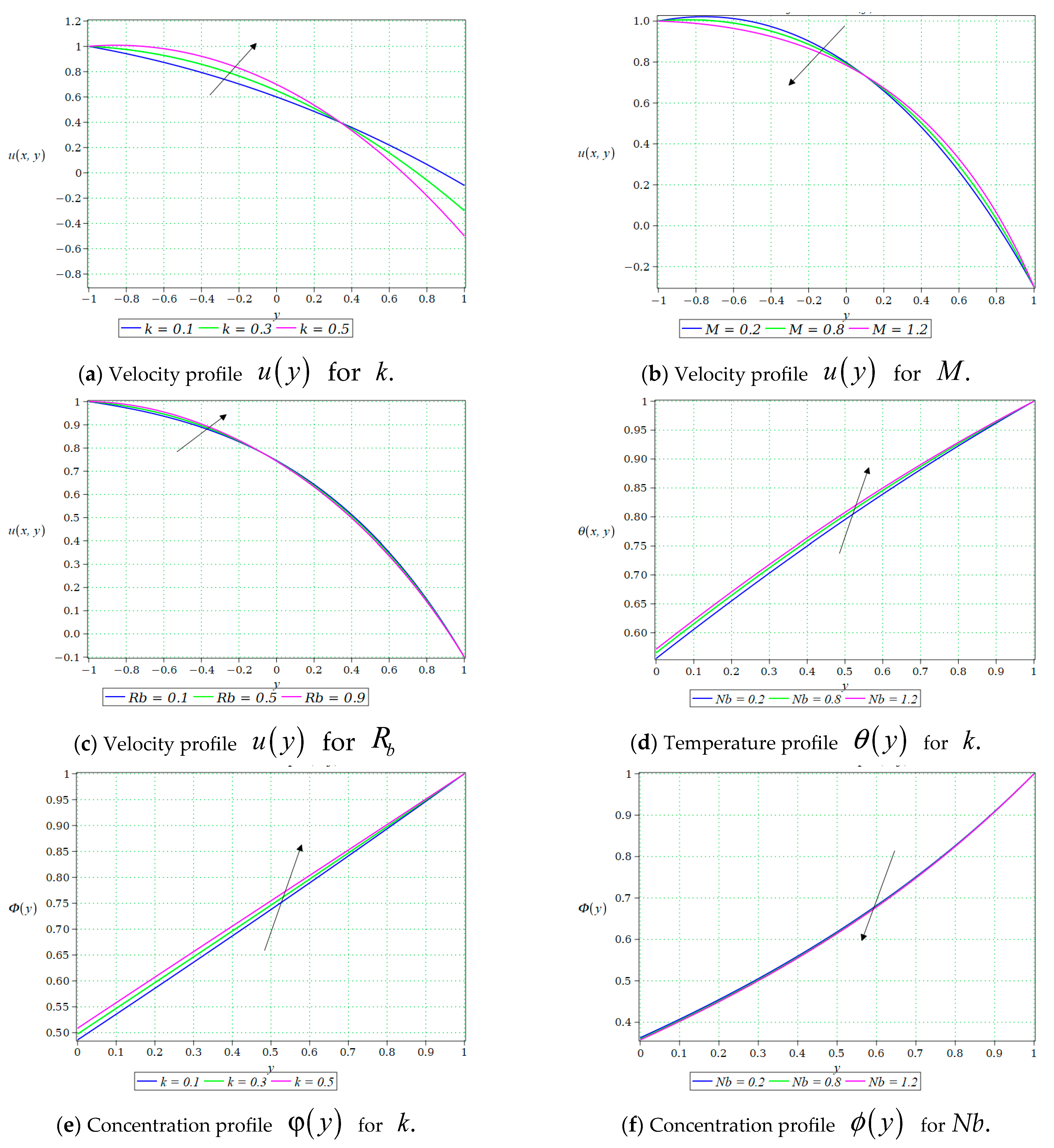
The discussion is based on the numerical results obtained for the Sutterby MHD nanofluid flowing in a thin channel formed by two counter-rotating rolls. The variations in velocity, temperature, concentration, and microorganism distributions are examined with respect to numerous governing parameters, and the outcomes are illustrated and interpreted through graphical representations. Figure 9, Figure 10 and Figure 11 provide valuable insights into the variations in dimensionless velocity, temperature, concentration, and microorganism distribution at the nip position $\left(x=0\right)$. Figure 9a presents the velocity profiles $u\left(y\right)$ for different values of the velocity ratio parameter $k=0.1,0.3,$ and $0.5$. As $k$ increases, the fluid velocity within the channel also increases, which is physically consistent since larger velocity ratios correspond to faster roll speeds and greater momentum transfer. The most significant variations occur in the near-wall regions, particularly close to the upper boundary. For smaller values of $k$ (e.g., $k=0.1$), the velocity decays more gradually, indicating weaker acceleration. In contrast, for higher values of $k$ (e.g., $k=0.5$), the profile shifts upward, demonstrating higher velocity magnitudes across most of the channel. Importantly, the maximum velocity is attained near the roll surfaces, where direct interaction with the moving rolls exerts the strongest influence on the fluid motion. Figure 9b illustrates the outcome of the magnetic parameter $M$ on the velocity profile $u\left(y\right)$ for $M=0.2,0.8,$ and 1.2. It is observed that as $M$ increases, the fluid velocity decreases throughout the channel. This trend is expected because a stronger magnetic field induces a Lorentz force, which acts as a resistive drag force opposing the motion of the electrically conducting nanofluid. Consequently, momentum transfer is suppressed, leading to a reduction in velocity. Similarly, Figure 9c shows the effect of the bioconvection parameter $R_b$ on the velocity profile u(y) for $R_b=0.1,0.5,$ and 0.9. It can be observed that increasing $R_b$ causes a rise in the fluid velocity across the channel.

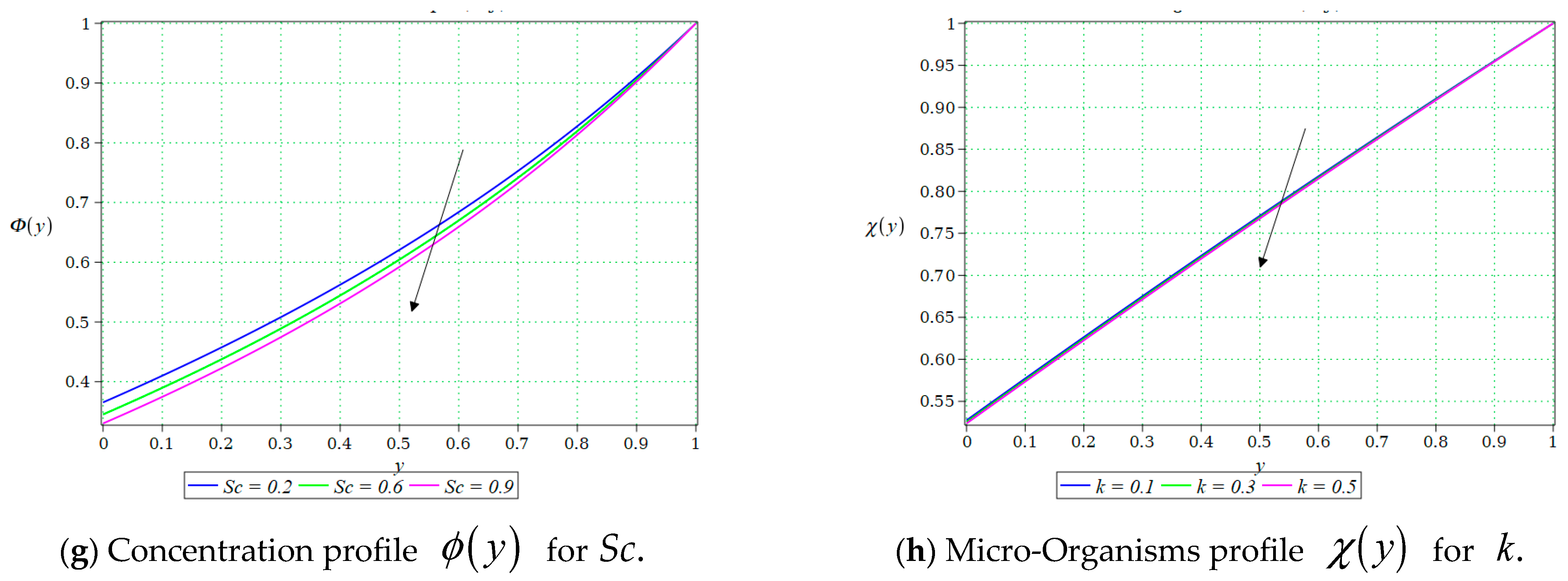
Figure 9e–g illustrates the nanoparticle concentration and micro-organism profiles under the influence of key flow parameters, namely the Brownian motion parameter, the velocity ratio parameter, and the Schmidt number. Figure 9e shows the outcome of the velocity ratio parameter $k$ on the nanoparticle concentration distribution $\varphi \left(y\right)$ across the channel. It is observed that as $k$ increases from 0.1 to 0.5, the concentration profile gradually shifts upward, leading to higher nanoparticle concentrations throughout the domain. Physically, a higher velocity ratio corresponds to stronger counter-rotating roll motion, which enhances fluid mixing and intensifies convective transport. Figure 9g demonstrates the impact of the Brownian motion parameter $Nb$ on the nanoparticle concentration profile $\varphi \left(y\right)$. As $Nb$ increases from 0.2 to 1.2, the concentration curves shift downward, indicating a reduction in nanoparticle concentration throughout the channel. This occurs because increased random motion causes nanoparticles to disperse more widely within the fluid, thereby lowering the concentration profiles.

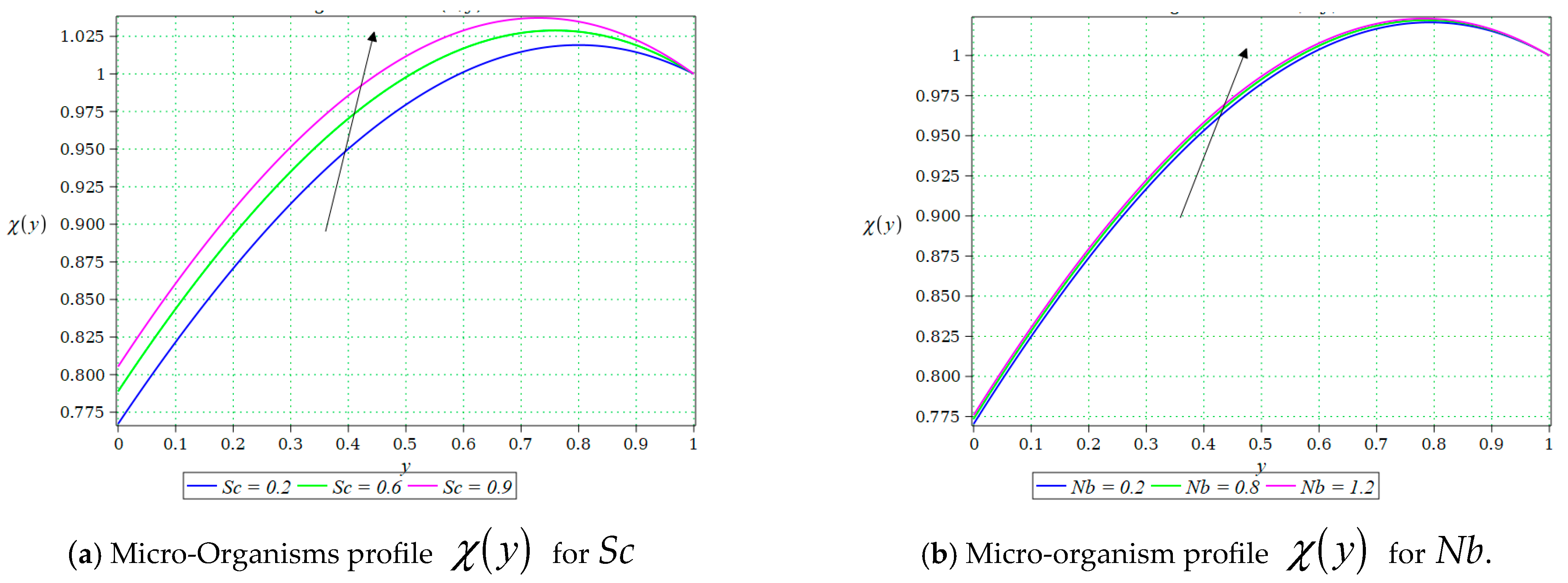
In the context of Sutterby nanofluid flow through reverse roll coating, microorganisms are important as their collective movement induces bioconvective effects that alter the fluid structure and flow characteristics. Their presence introduces additional dynamics into the system, making them a valuable factor to consider in analyzing coating processes. Figure 9h and Figure 10a,b demonstrates the sensitivity of the Micro-Organisms profile $\chi \left(y\right)$ to variations in key dimensionless parameters, namely the velocity ratio parameter $k$, the Schmidt number $Sc$, the Brownian motion parameter $Nb$ and Peclet number $Pe$. Figure 10a highlights the role of the velocity ratio parameter $k$ on the microorganism distribution profile. The concentration profiles have decreasing trend for $k=0.1,0.3,$ and 0.5. Figure 10b illustrates the impact of the Schmidt number $Sc$, on the Micro-Organisms profile $\chi \left(y\right)$. As $Sc$ increases from 0.2 to 0.9, the microorganism concentration rises across the channel, with the profiles shifting upward. Figure 10b shows the impact of the Brownian motion parameter $Nb$ on the microorganism profile $\chi \left(y\right)$. It is observed that increasing $Nb$ from 0.2 to 0.9 elevates the microorganism profile. The trend suggests that enhanced nanoparticle random motion indirectly promotes microorganism distribution.

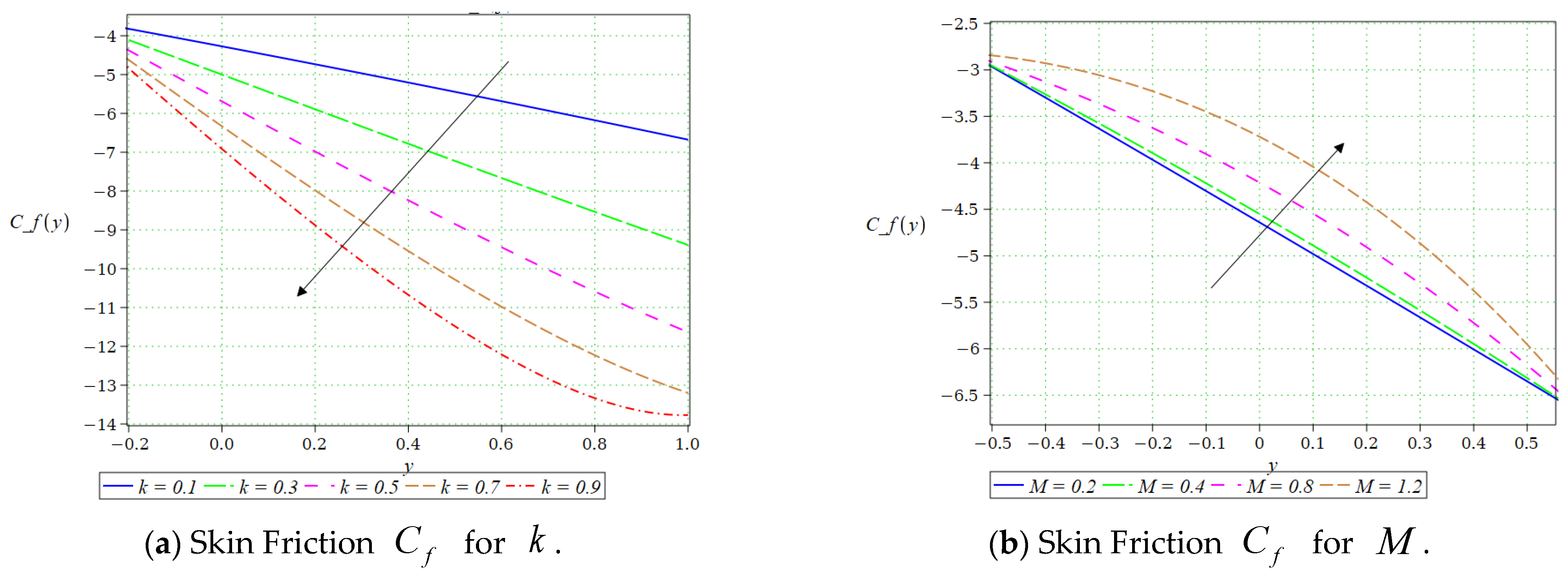
Skin friction is a fundamental engineering quantity in analyzing non-Newtonian nanofluid flow through the reverse roll coating process. It quantifies the shear stress exerted by the fluid at the roll surfaces, which directly governs the energy required to drive the rolls and plays a vital role in maintaining the stability and uniformity of the coating layer. The impact of various parameters on the skin friction coefficient is presented in Figure 11a–e. The influence of the $k$ is shown in Figure 11a. As $k$ increases from 0.1 to 0.9, the skin friction coefficient decreases significantly, with the profiles shifting downward. Figure 11b illustrates the effect of the magnetic field parameter $M$, where an increase in $M$ reduces the magnitude of skin friction due to the Lorentz forces opposing the fluid motion and thereby enhancing resistance near the wall. The variation with the Brownian motion parameter $Nb$ is shown in Figure 11c, where increasing $Nb$ from 0.2 to 1.2, results in a slight reduction in skin friction. A similar trend is observed for the bioconvection number $R_b$ in Figure 11d, indicating a modest decrease in skin friction with increasing microorganism activity. Finally, Figure 11e depicts the effect of the Schmidt number $Sc$, where increasing Sc from 0.2 to 1.0 produces a gradual decline in the skin friction coefficient. In the next phase, we extend the analysis to heat transfer characteristics, where the predictive capabilities of the ANN-LMA framework are discussed in detail.

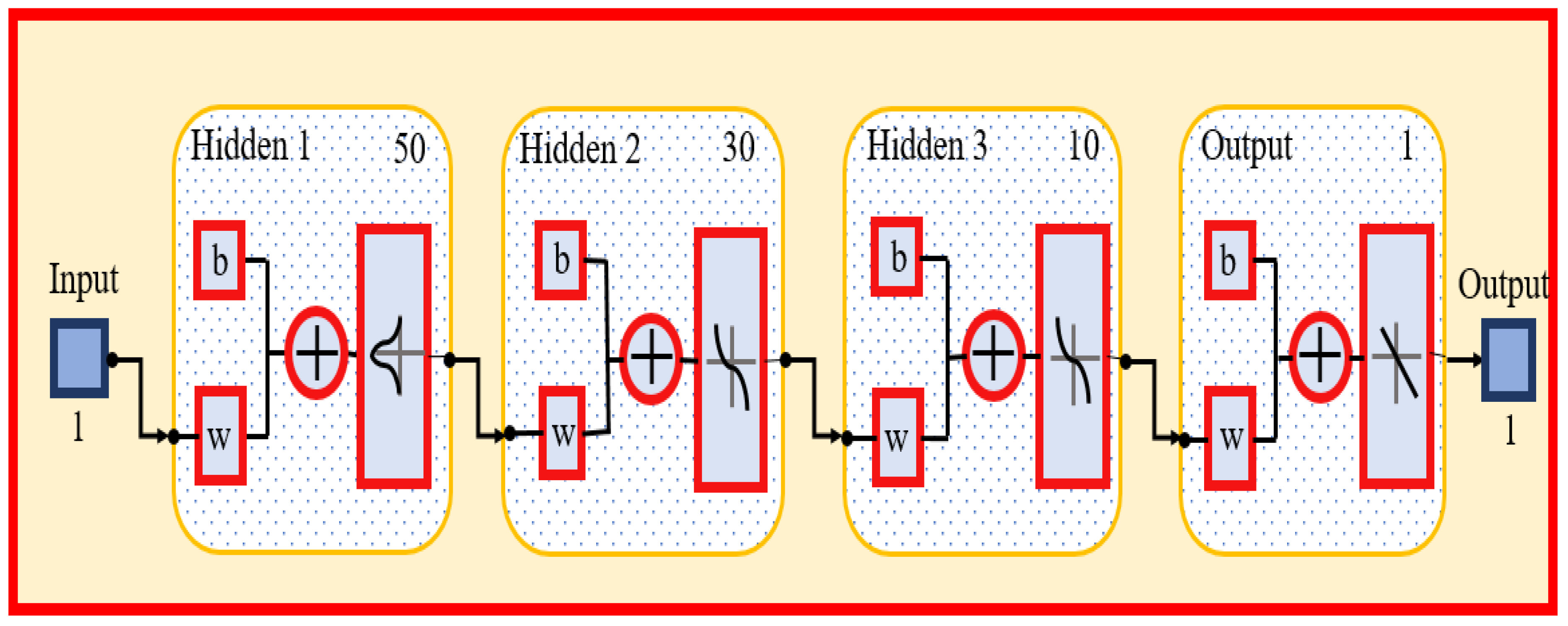
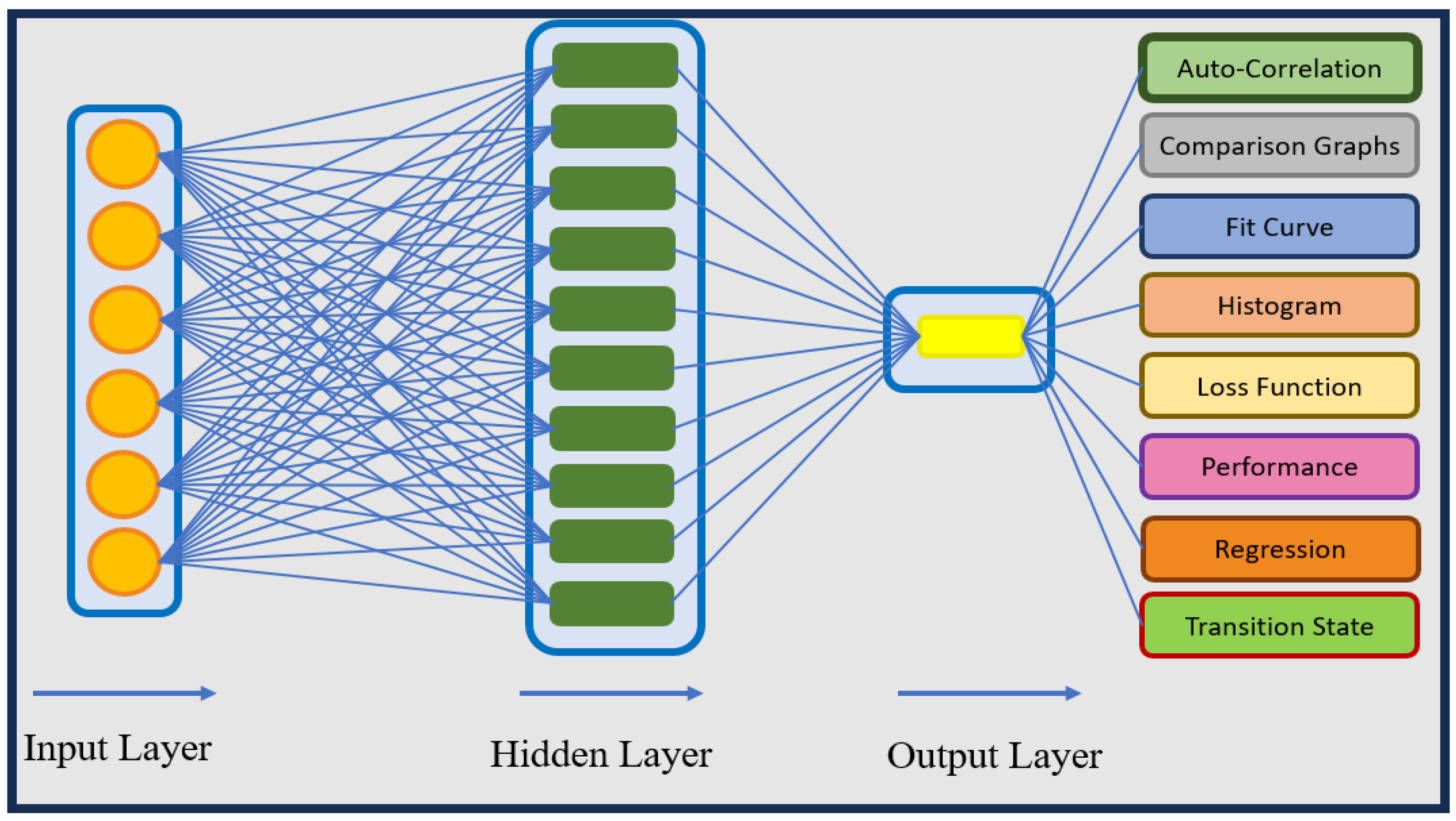
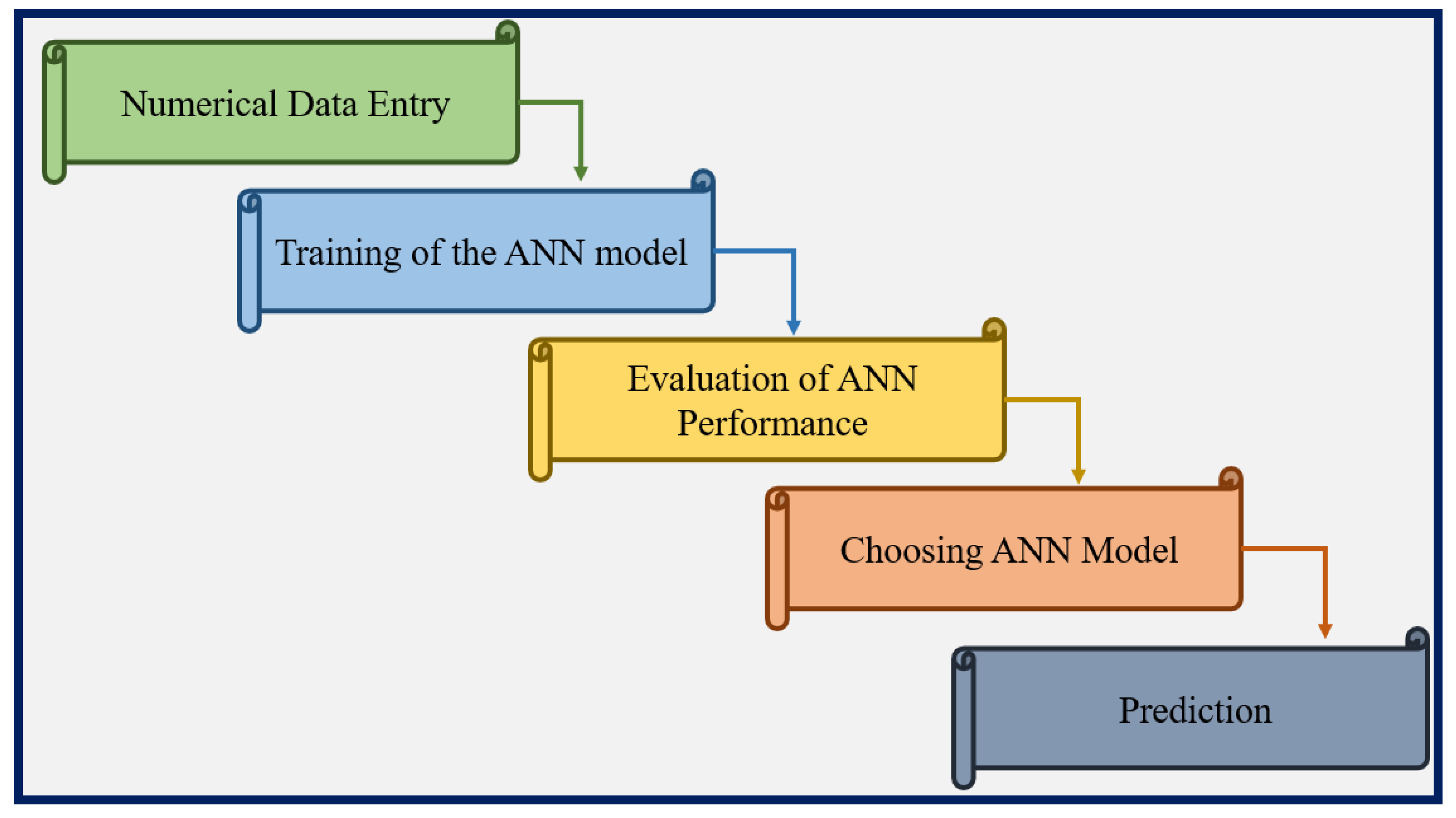
ANNs-LMA Discussion

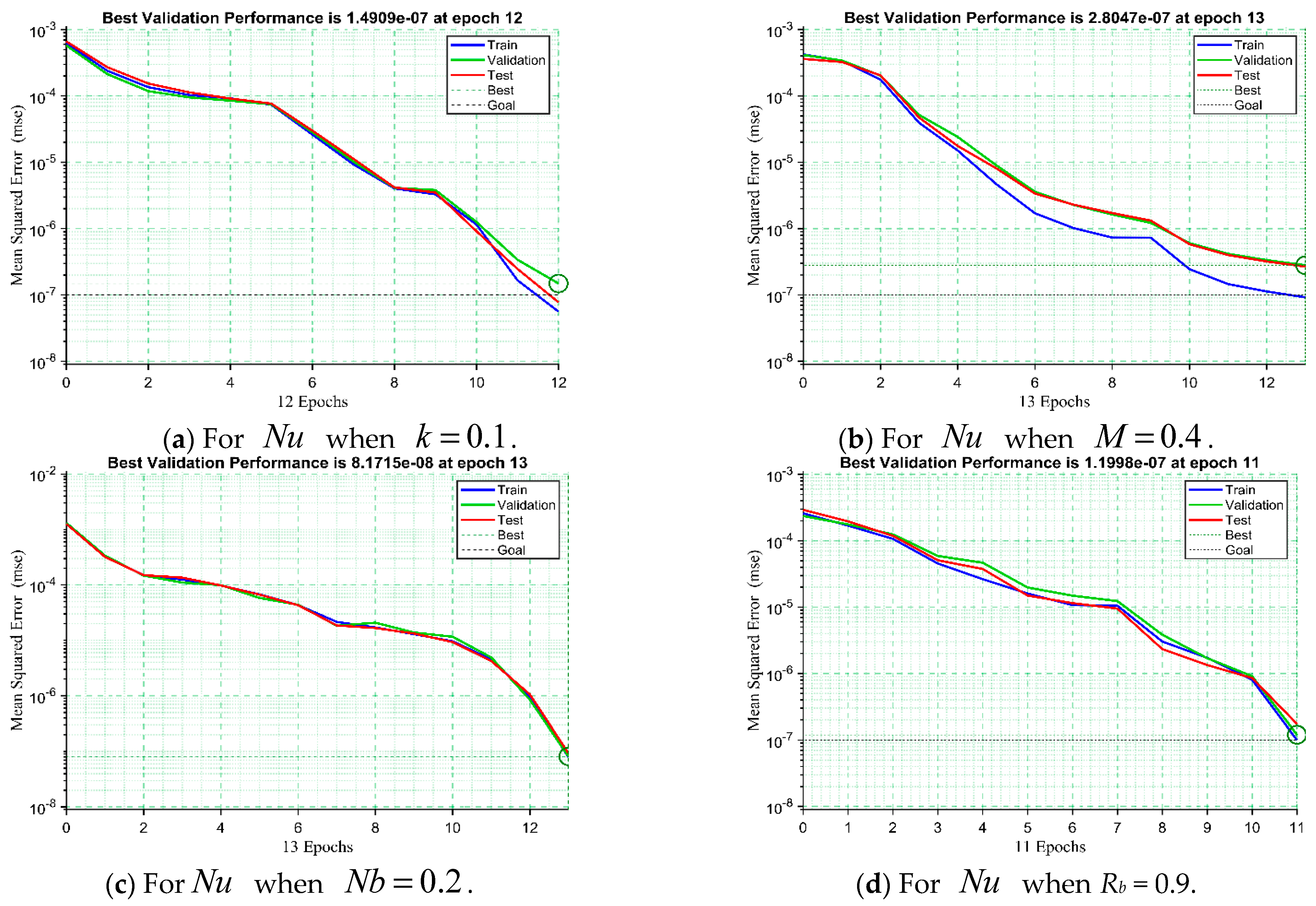
Now we will discuss the output of the ANNs-LMB for heat transfer in the Sutterby MHD nanofluid within a thin channel. Figure 12, Figure 13, Figure 14, Figure 15, Figure 16, Figure 17, Figure 18 and Figure 19 present the outcomes of ANNs-LMB, including performance, histogram, MSE, loss function, and comparisons across training, validation, and testing under different scenarios. Figure 12a–d demonstrates the performance of the ANNs-LMB models through the MSE trajectories obtained during training, validation, and testing across different scenarios. As observed, all models demonstrate rapid convergence toward very low error values, with the optimal validation performance attained at specific epochs. In particular, the MSE curves highlight the convergence patterns of the trained datasets, where the best validation performances are recorded as $1.4909\times {10}^{-7}$ epoch 12, $2.8047\times {10}^{-7}$ at epoch 13, $8.1715\times {10}^{-8}$ at epoch 13, and $1.1998\times {10}^{-7}$ at epoch 11. The smooth decline and close alignment of the training, validation, and testing curves confirm the efficient learning capability of the models and their robustness in generalization, with minimal signs of overfitting. These results emphasize the reliability and adaptability of ANNs-LMA in capturing the highly nonlinear interactions governing the nanofluid system.

Figure 13a–d presents the error histograms for various scenarios of Nusselt number prediction in the thin channel using the ANNs-LMA model. The horizontal axis represents the error values, calculated as the difference between targets and outputs (Errors = Targets − Outputs), while the vertical axis shows the number of instances (frequency) corresponding to each error bin. Each histogram is divided into 20 bins, with blue, green, and red bars denoting the training, validation, and testing datasets, respectively. The vertical orange line indicates the position of zero error, serving as the reference for perfect prediction. From the figure, it can be observed that most of the errors are concentrated close to zero, representing strong model accuracy and only slight deviation from the actual values. The symmetry distribution reveals the absence of significant bias, suggesting that the models perform consistently well across all datasets. This consistency highlights their robust ability to simplify with minimal risk of overfitting. Across all scenarios, the majority of errors are distributed tightly around the zero line, confirming that the model has achieved highly accurate predictions with minimal deviation. In the first case, the maximum concentration of instances is centered between approximately $-2.0\times {10}^{-4}$ and $2.0\times {10}^{-4}$, with the highest frequency exceeding 300 instances. Similarly, in the second scenario, the errors cluster within the range of about $-4.0\times {10}^{-4}$ and $4.0\times {10}^{-4}$, with the tallest bin reaching nearly 200 instances. Based on these outcomes, it can be concluded that the ANNs-LMA model maintains stable and reliable performance across validation, training, and testing phases. 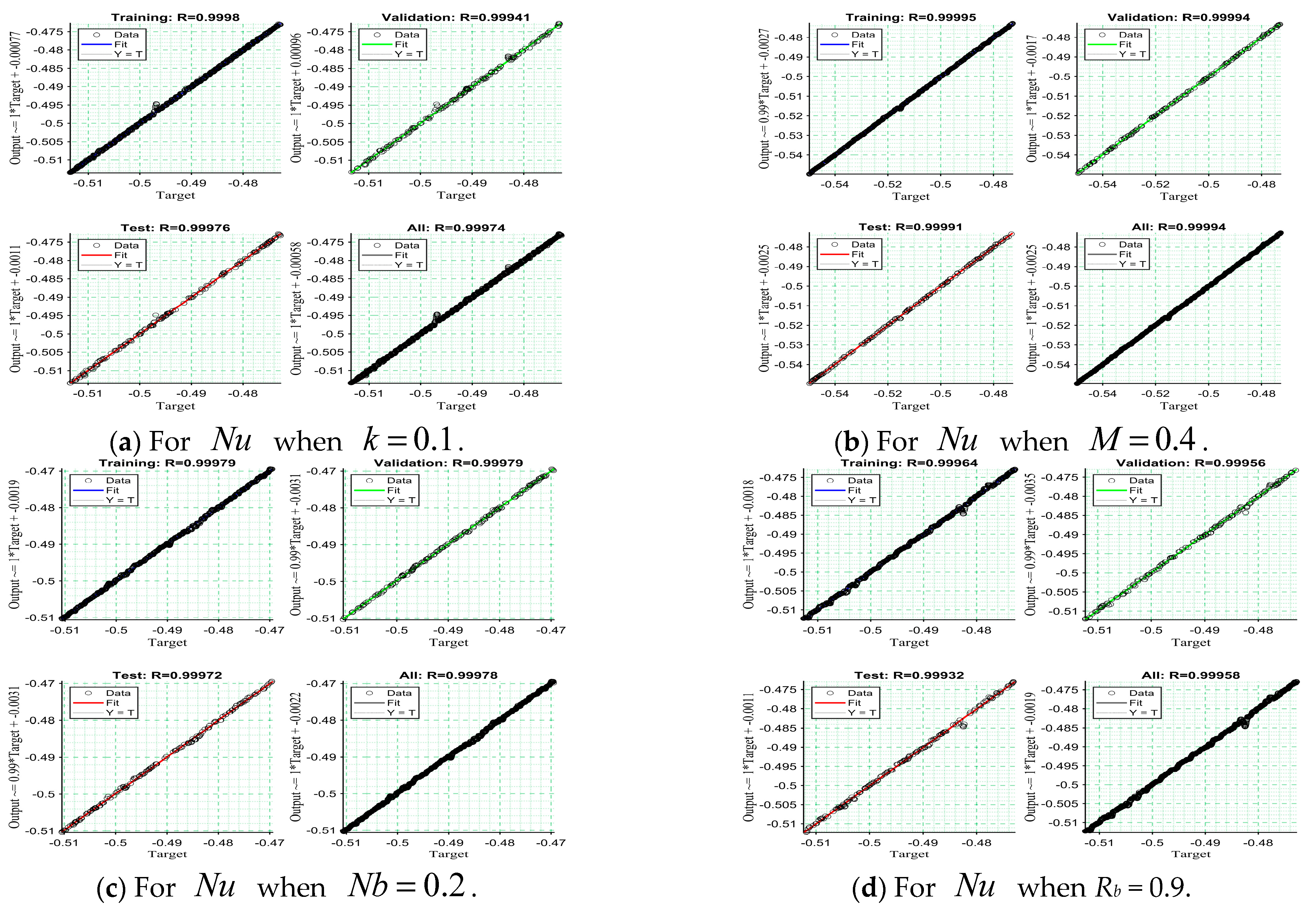Figure 14a–d presents the regression plots of the ANN models for the training, validation, and testing phases, highlighting the correlation between the actual and predicted outputs. In all cases, the data points lie very close to the best-fit line (Y = T), with correlation coefficients $(R)$ exceeding 0.999, which reflects a near-perfect agreement between predictions and targets. Such consistently high $R$-values demonstrate the reliability of the model in capturing the underlying nonlinear dynamics of the system. The strong linear alignment observed across all phases further confirms the absence of overfitting, emphasizing the model’s capability to generalize effectively across different datasets.

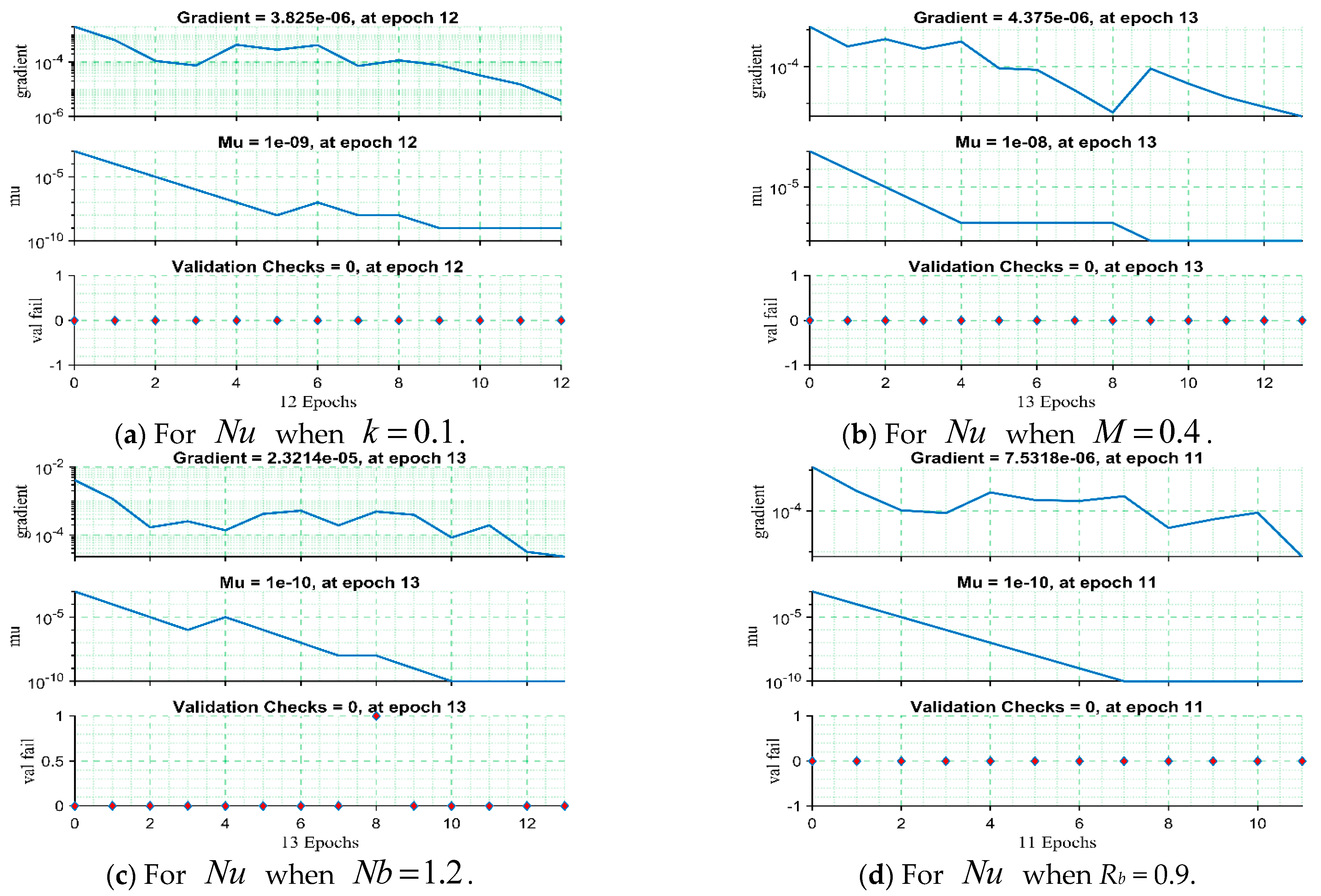
The training performance of ANNs-LMA models for multiple output parameters across distinct physical scenarios is presented in Figure 15a–d. The figures highlight significant training characteristics such as gradient values, $Mu$ parameter variation, and validation tests. In all cases, the gradient values decrease steadily with training, reaching very small magnitudes, which indicates effective convergence and error minimization. The $Mu$ parameters also decline consistently, reflecting stable adjustments of the learning process and consistent improvements in training. Notably, the validation checks remain at zero throughout, confirming that no validation failures occurred and demonstrating the model’s strong ability to avoid overfitting. These observations jointly validate the efficiency, accuracy, and dependability of the ANNs-LMA models in capturing the nonlinear system behavior, while the rapid convergence within 11–13 epochs further emphasizes the robustness and reliability of the training process. 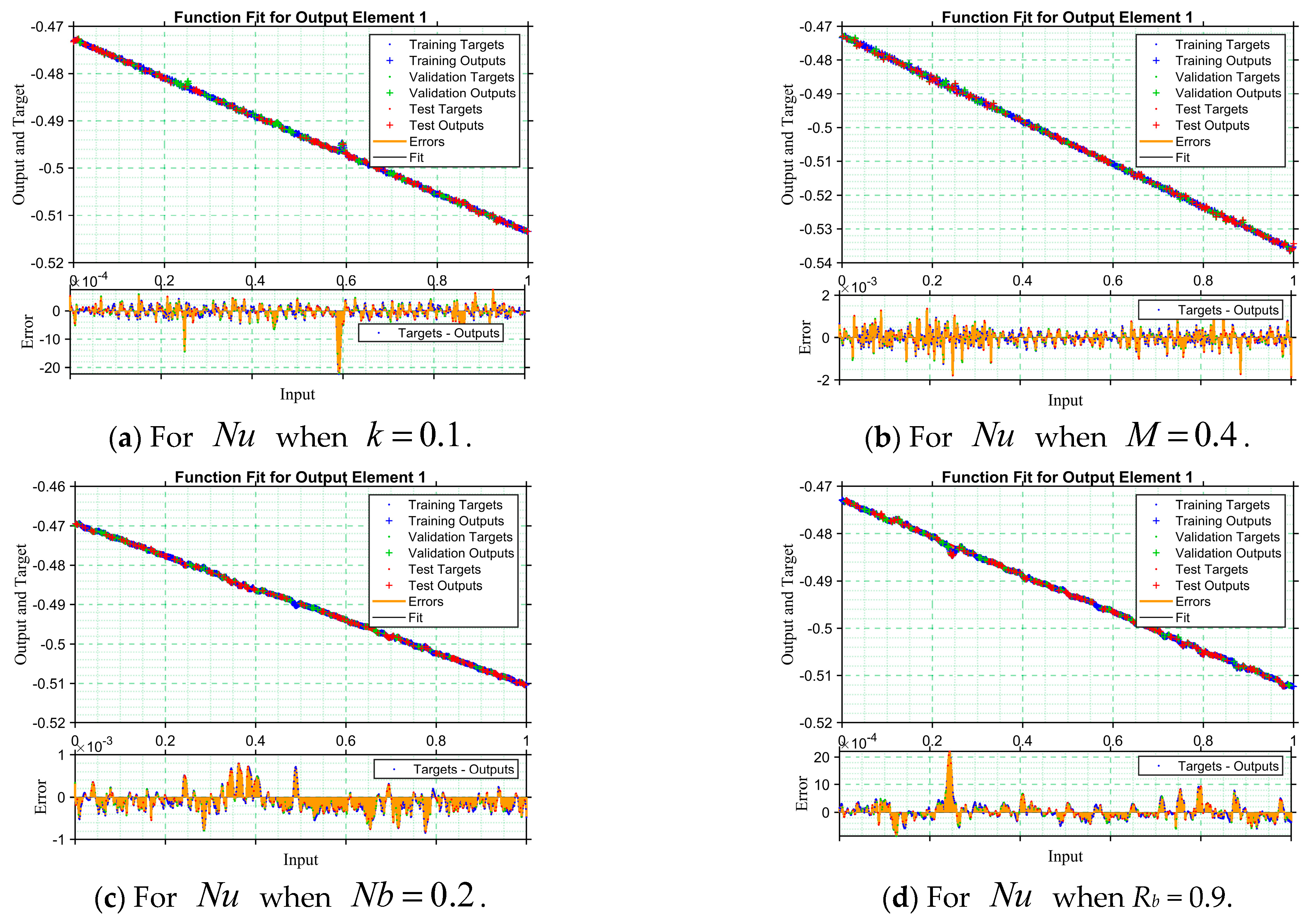Furthermore, Figure 16a–d presents the function fit plots for the trained ANNs-LMA models, where training, validation, and testing datasets are represented by blue, green, and red points, respectively. The black line represents the best-fit curve, whereas the orange line demonstrates the prediction error. In all cases, the predicted outputs align very closely with the target values, demonstrating strong model accuracy. The error plots below each fit confirm this performance, with most errors concentrated around zero. In Figure 16a, errors fluctuate within a narrow range of approximately -0.001 to 0.001, indicating negligible deviation. In Figure 16b, the errors spread slightly wider, ranging between −0.002 and 0.002. Similarly, Figure 16c, d shows minimal deviations, with error values confined to small magnitudes without large outliers.

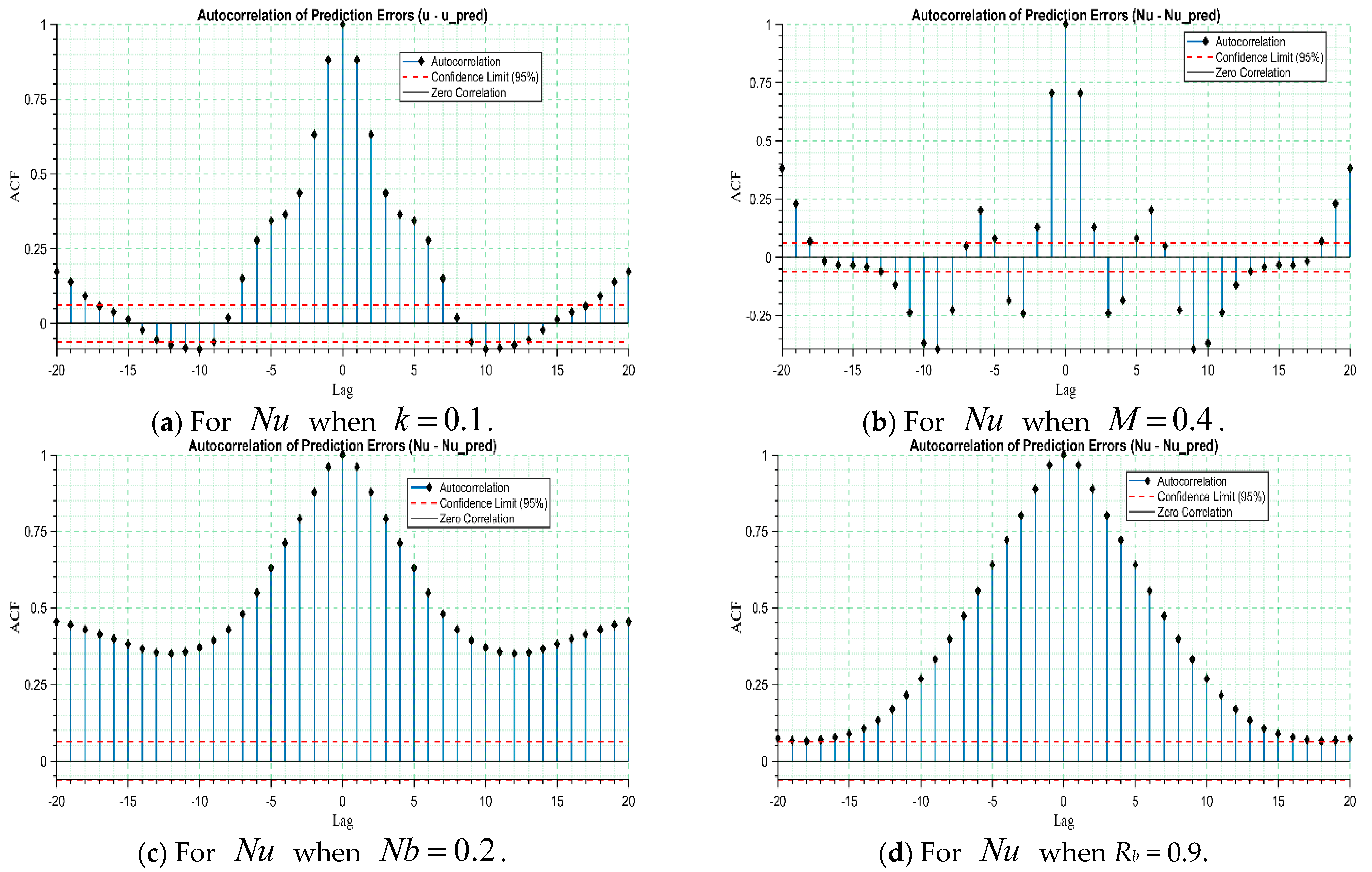
Next, we present the autocorrelation error plots for different scenarios, which are used to evaluate the independence of residual errors in the ANNs-LM model. Ideally, prediction errors should be uncorrelated and lie within the 95% confidence bounds, indicating that the model has efficiently captured the underlying data patterns without leaving systematic dependencies. The autocorrelation error analysis for each scenario of the proposed model trained using the solver is shown in Figure 17a–d. In these cases, most spikes remain within or close to the confidence limits, suggesting that the residuals are largely uncorrelated and that the ANN provides reliable predictions.

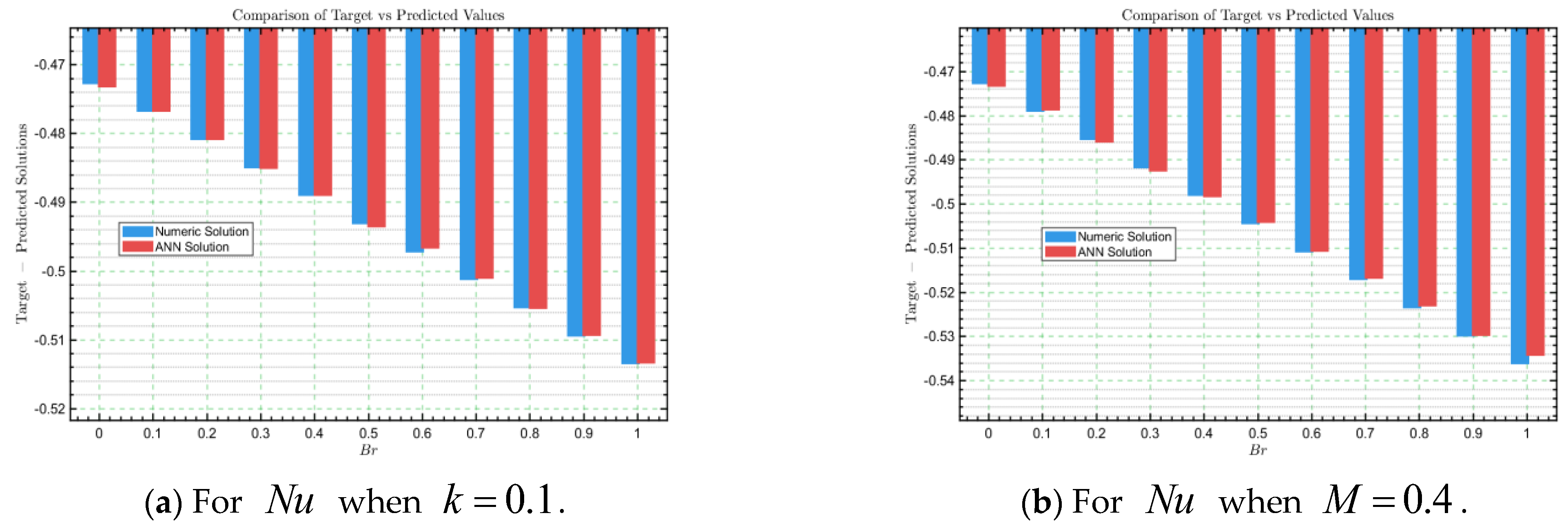
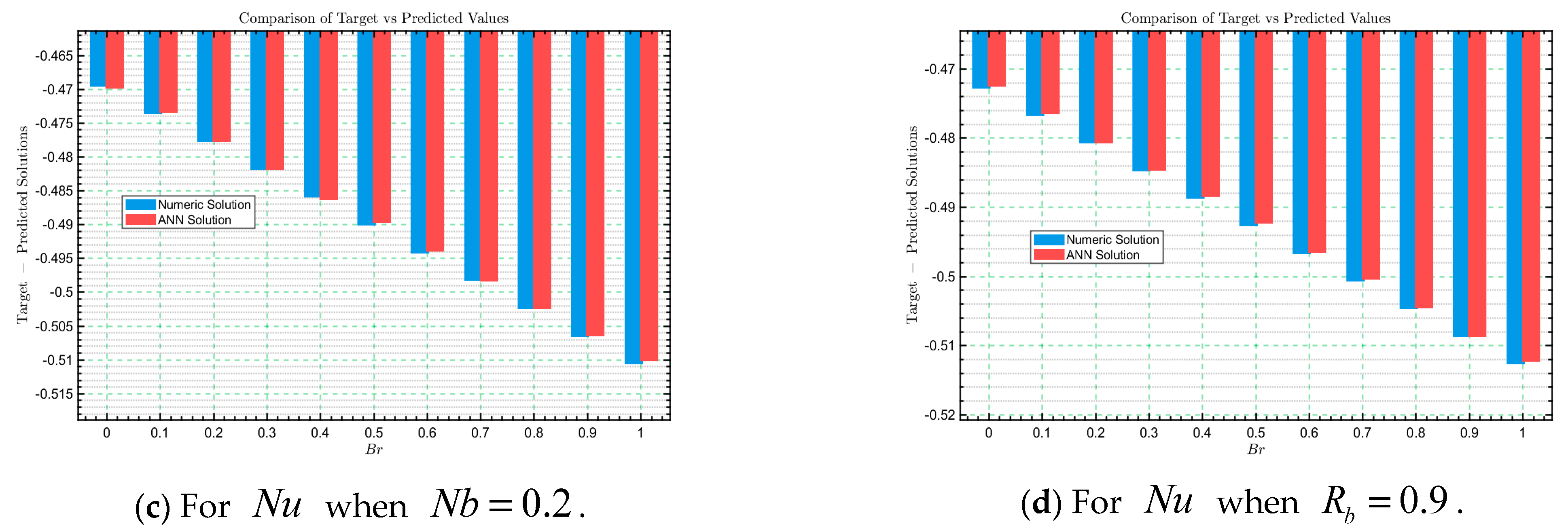
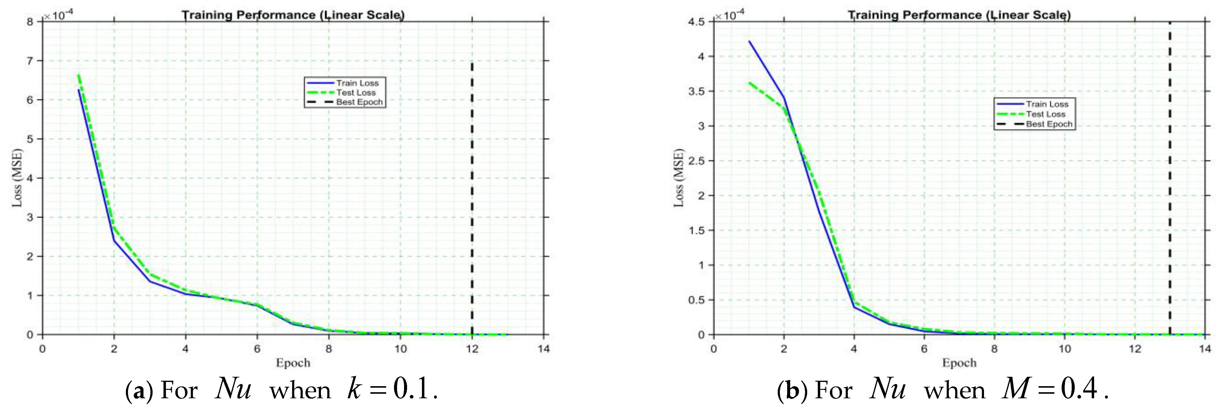
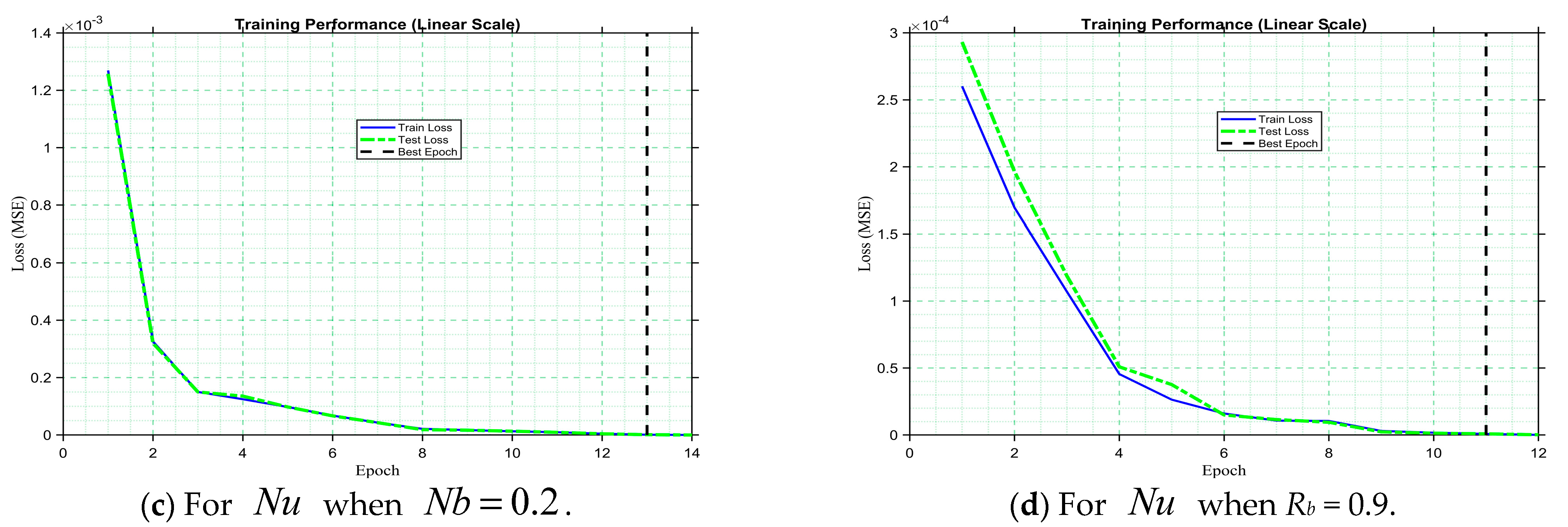
The comparison between numerical solutions and ANNs-LMA predicted solutions is essential for validating the reliability of the trained model. Figure 18a–d presents bar plots that compare the target (numeric) and predicted (ANNs-LMA) solutions versus the Brinkman number (Br) on the horizontal axis and the predicted solution on the vertical axis. In each case, the ANNs-predicted values closely follow the numeric solutions with only minor deviations, demonstrating excellent agreement. This strong alignment confirms that the ANNs-LMA model successfully captures the underlying physical behavior of the system and can serve as a dependable surrogate to traditional numerical methods. Such comparison is important as it not only verifies prediction accuracy but also establishes the ANN model’s potential for computational efficiency in complex fluid dynamic problems. Moreover, the evaluation of the training and testing loss functions is equally important to assess the stability and convergence of the ANNs-LMA model. Figure 19a–d displays the loss (MSE) versus epochs, showing a rapid decrease in error during the initial iterations followed by stabilization at very low values $\left({10}^{-4}-{10}^{-5}\right)$. The close overlap of training and testing loss curves indicates that the model has converged efficiently without signs of overfitting or underfitting. This behavior highlights the robustness of the ANNs-LMA in generalizing across unseen data and achieving reliable predictive performance. The consistent minimization of the loss function demonstrates that the ANNs-LMA model not only reproduces the numerical results accurately but also ensures long-term stability and efficiency in practical prediction tasks.

The convergence performance of the developed ANNs-LMA model has been evaluated using statistical measures such as performance, MSE, gradient, mu, validation, and epochs under varying parametric conditions ($k,M,Nb$ and $R_b$). The results summarized in

Table 2. Numerical analysis for the Temperature of ANNs-LMA for the parameter $k$.

k	MSE		Performance	Gradient	Mu	Validation	Epoch
	Train Value	Testing Value
0.1	$5.6119\times {10}^{-8}$	$7.7549\times {10}^{-8}$	$1.4909\times {10}^{-7}$	$3.835\times {10}^{-6}$	$1\times {10}^{-9}$	$6.1469\times {10}^{-8}$	12
0.3	$9.118\times {10}^{-8}$	$5.4563\times {10}^{-7}$	$6.9617\times {10}^{-7}$	$3.6602\times {10}^{-6}$	$1\times {10}^{-8}$	$2.8047\times {10}^{-7}$	12
0.7	$9.0275\times {10}^{-8}$	$4.7891\times {10}^{-7}$	$5.5392\times {10}^{-7}$	$2.9167\times {10}^{-6}$	$1\times {10}^{-8}$	$7.1993\times {10}^{-8}$	16
0.9	$6.7095\times {10}^{-8}$	$1.3277\times {10}^{-7}$	$1.2998\times {10}^{-7}$	$2.1715\times {10}^{-5}$	$1\times {10}^{-9}$	$4.2398\times {10}^{-7}$	14

,

Table 3. Numerical analysis for the velocity of ANNs-LMA for the parameter $M$.

M	MSE		Performance	Gradient	Mu	Validation	Epoch
	Train Value	Testing Value
0.2	$2.8488\times {10}^{-8}$	$6.5269\times {10}^{-8}$	$6.1469\times {10}^{-8}$	$7.9863\times {10}^{-6}$	$1\times {10}^{-9}$	$6.1469\times {10}^{-8}$	11
0.4	$9.2097\times {10}^{-8}$	$2.6757\times {10}^{-7}$	$2.8047\times {10}^{-7}$	$4.375\times {10}^{-6}$	$1\times {10}^{-8}$	$2.8047\times {10}^{-7}$	13
0.8	$6.5293\times {10}^{-8}$	$1.0558\times {10}^{-7}$	$7.1993\times {10}^{-8}$	$1.5918\times {10}^{-5}$	$1\times {10}^{-10}$	$7.1993\times {10}^{-8}$	13
1.2	$8.1761\times {10}^{-8}$	$4.0553\times {10}^{-7}$	$4.2398\times {10}^{-7}$	$8.891\times {10}^{-6}$	$1\times {10}^{-8}$	$4.2398\times {10}^{-7}$	13

,

Table 4. Numerical analysis for the temperature of ANNS-LMA for the parameter $Nb$.

Nb	MSE		Performance	Gradient	Mu	Validation	Epoch
	Train Value	Testing Value
0.2	$7.8796\times {10}^{-8}$	$9.3222\times {10}^{-8}$	$8.1715\times {10}^{-8}$	$2.3214\times {10}^{-5}$	$1\times {10}^{-10}$	$8.1715\times {10}^{-8}$	13
0.4	$4.6451\times {10}^{-8}$	$1.5018\times {10}^{-7}$	$1.1865\times {10}^{-7}$	$1.6417\times {10}^{-5}$	$1\times {10}^{-9}$	$1.1865\times {10}^{-7}$	10
0.8	$3.8563\times {10}^{-8}$	$9.1904\times {10}^{-8}$	$7.2229\times {10}^{-8}$	$4.3947\times {10}^{-6}$	$1\times {10}^{-9}$	$7.2229\times {10}^{-8}$	15
1.2	$1.3758\times {10}^{-8}$	$2.3738\times {10}^{-8}$	$2.6968\times {10}^{-8}$	$5.6077\times {10}^{-6}$	$1\times {10}^{-10}$	$2.6968\times {10}^{-8}$	11

and

Table 5. Numerical analysis for the velocity of ANNS-LMA for the parameter $R_b$.

${\mathit{R}}_{\mathit{b}}$	MSE		Performance	Gradient	Mu	Validation	Epoch
	Train Value	Testing Value
0.1	$6.7757\times {10}^{-8}$	$8.2552\times {10}^{-8}$	$7.1469\times {10}^{-8}$	$1.2605\times {10}^{-5}$	$1\times {10}^{-10}$	$7.1469\times {10}^{-8}$	14
0.5	$3.3512\times {10}^{-8}$	$6.6279\times {10}^{-8}$	$6.0018\times {10}^{-8}$	$2.7317\times {10}^{-5}$	$1\times {10}^{-10}$	$6.0018\times {10}^{-8}$	13
0.7	$6.6256\times {10}^{-8}$	$1.412\times {10}^{-7}$	$1.164\times {10}^{-7}$	$2.105\times {10}^{-5}$	$1\times {10}^{-9}$	$1.164\times {10}^{-7}$	10
0.9	$9.9798\times {10}^{-8}$	$1.6351\times {10}^{-7}$	$1.1998\times {10}^{-7}$	$7.5318\times {10}^{-6}$	$1\times {10}^{-10}$	$1.1998\times {10}^{-7}$	11

highlight that the model consistently achieves low MSE values across both training and testing datasets. For example, at $k=0.1$, the training and testing MSE values are $5.6119\times {10}^{-8}$ and $7.7549\times {10}^{-8}$, respectively, with a performance value of $1.4909\times {10}^{-7}$ and a gradient of $3.835\times {10}^{-6}$ within 12 epochs. Similarly, at $M=0.2$, the model converges with training and testing MSE values of $2.8488\times {10}^{-8}$ and $6.5269\times {10}^{-8}$, achieving performance of $6.1469\times {10}^{-8}$ and a gradient of $7.9863\times {10}^{-6}$ after only 11 epochs. For the case of $Nb=0.4$, the ANN-LMA demonstrates training and testing MSE values of $3.8563\times {10}^{-8}$ and $9.1904\times {10}^{-8}$, with a performance of 7.2229 × 10⁻⁸ and a gradient of $4.3947\times {10}^{-6}$ over 15 epochs. Similarly, the results for the bioconvection number $R_b$ can be observed from Table 5, where the ANN-LMA model again exhibits stable convergence behavior with low training and testing MSE values, controlled gradients, and efficient epochs. Across all cases, the gradients gradually reduce to the order of ${10}^{-6}-{10}^{-5}$, while the mu parameter remains stable between ${10}^{-8}$ and ${10}^{-10}$, reflecting robust convergence. The validation values remain close to the training accuracy, and the required epochs (ranging between 10 and 16) further confirm efficient convergence without excessive iterations. These outcomes demonstrate that the ANN-LMA model not only reproduces the numerical solutions with high accuracy but also ensures computational efficiency and strong adaptability to capture the nonlinear dynamics of the system under diverse fluid flow scenarios.

Assessing multiple statistical error metrics is important to validate the reliability and robustness of the ANNs-LMB model under varying physical parameters. The outcomes presented in

Table 6. Impact of the $k$ on the $Nu$.

k	MAE	MSE	RMSE	ME	MAD	R2	SST	SSR	Mean AE
0.1	$1.7\times {10}^{-4}$	$7.33\times {10}^{-8}$	$2.71\times {10}^{-8}$	$-3.21\times {10}^{-6}$	$1.72\times {10}^{-4}$	$9.10\times {10}^{-1}$	$1.39\times {10}^{-1}$	$7.34\times {10}^{-5}$	$3.47\times {10}^{-4}$
0.3	$3.1\times {10}^{-4}$	$2.50\times {10}^{-7}$	$4.50\times {10}^{-8}$	$1.78\times {10}^{-5}$	$3.10\times {10}^{-4}$	$9.96\times {10}^{-1}$	$5.21\times {10}^{-1}$	$2.50\times {10}^{-4}$	$6.05\times {10}^{-4}$
0.7	$3.2\times {10}^{-4}$	$2.18\times {10}^{-7}$	$4.67\times {10}^{-8}$	$-1.15\times {10}^{-5}$	$3.16\times {10}^{-4}$	$9.10\times {10}^{-1}$	$1.922$	$2.19\times {10}^{-4}$	$5.77\times {10}^{-4}$
0.9	$2.2\times {10}^{-4}$	$8.64\times {10}^{-8}$	$2.94\times {10}^{-8}$	$2.67\times {10}^{-5}$	$2.22\times {10}^{-4}$	$9.10\times {10}^{-1}$	$2.869$	$8.64\times {10}^{-5}$	$4.02\times {10}^{-4}$

,

Table 7. Impact of the $M$ on the $Nu$.

M	MAE	MSE	RMSE	ME	MAD	R2	SST	SSR	Mean AE
0.2	$1.54\times {10}^{-4}$	$3.89\times {10}^{-8}$	$1.98\times {10}^{-4}$	$2.36\times {10}^{-5}$	$1.52\times {10}^{-4}$	$9.10\times {10}^{-1}$	$3.00\times {10}^{-1}$	$3.90\times {10}^{-5}$	$3.09\times {10}^{-4}$
0.4	$2.85\times {10}^{-4}$	$1.47\times {10}^{-7}$	$3.83\times {10}^{-4}$	$-1.71\times {10}^{-5}$	$2.85\times {10}^{-4}$	$9.10\times {10}^{-1}$	$3.36\times {10}^{-1}$	$1.47\times {10}^{-4}$	$5.67\times {10}^{-4}$
0.6	$2.07\times {10}^{-4}$	$7.23\times {10}^{-8}$	$2.69\times {10}^{-4}$	$-2.87\times {10}^{-5}$	$2.00\times {10}^{-4}$	$9.10\times {10}^{-1}$	$4.95\times {10}^{-1}$	$7.24\times {10}^{-5}$	$3.99\times {10}^{-4}$
0.8	$2.04\times {10}^{-4}$	$7.23\times {10}^{-8}$	$2.69\times {10}^{-4}$	$-2.87\times {10}^{-5}$	$2.00\times {10}^{-4}$	$9.10\times {10}^{-1}$	$4.95\times {10}^{-1}$	$7.240\times {10}^{-5}$	$3.99\times {10}^{-4}$
1.2	$2.94\times {10}^{-4}$	$1.82\times {10}^{-7}$	$4.26\times {10}^{-4}$	$4.18\times {10}^{-5}$	$2.93\times {10}^{-4}$	$9.10\times {10}^{-1}$	$8.00\times {10}^{-1}$	$1.81\times {10}^{-4}$	$5.62\times {10}^{-4}$

,

Table 8. Impact of the $Nb$ on the $Nu$.

$\mathit{N}\mathit{b}$	MAE	MSE	RMSE	ME	MAD	${\mathit{R}}^2$	SST	SSR	MRE
0.2	$2.32\times {10}^{-4}$	$8.14\times {10}^{-8}$	$2.85\times {10}^{-4}$	$-1.30\times {10}^{-4}$	$1.86\times {10}^{-4}$	$9.10\times {10}^{-1}$	$1.41\times {10}^{-1}$	$8.15\times {10}^{-5}$	$4.73\times {10}^{-1}$
0.4	$1.95\times {10}^{-4}$	$7.28\times {10}^{-8}$	$2.70\times {10}^{-4}$	$8.80\times {10}^{-5}$	$1.82\times {10}^{-4}$	$9.10\times {10}^{-1}$	$1.39\times {10}^{-1}$	$7.29\times {10}^{-5}$	$4.04\times {10}^{-1}$
0.8	$1.69\times {10}^{-4}$	$5.16\times {10}^{-8}$	$2.22\times {10}^{-4}$	$7.30\times {10}^{-6}$	$1.66\times {10}^{-4}$	$9.10\times {10}^{-1}$	$1.37\times {10}^{-1}$	$5.17\times {10}^{-5}$	$3.54\times {10}^{-1}$
1.2	$9.20\times {10}^{-4}$	$1.72\times {10}^{-8}$	$1.31\times {10}^{-4}$	$2.90\times {10}^{-5}$	$8.95\times {10}^{-5}$	$9.10\times {10}^{-1}$	$1.35\times {10}^{-1}$	$1.73\times {10}^{-5}$	$2.02\times {10}^{-1}$

and

Table 9. Impact of the $R_b$ on the $Nu$.

${\mathit{R}}_{\mathit{b}}$	MAE	MSE	RMSE	ME	MAD	R2	SST	SSR	Mean AE
0.1	$1.97\times {10}^{-4}$	$7.05\times {10}^{-8}$	$2.69\times {10}^{-4}$	$1.23\times {10}^{-4}$	$1.68\times {10}^{-4}$	$9.10\times {10}^{-1}$	$1.42\times {10}^{-1}$	$7.06\times {10}^{-5}$	$4.00\times {10}^{-4}$
0.5	$1.69\times {10}^{-4}$	$4.24\times {10}^{-8}$	$2.06\times {10}^{-4}$	$1.51\times {10}^{-4}$	$9.24\times {10}^{-5}$	$9.10\times {10}^{-1}$	$1.36\times {10}^{-1}$	$4.24\times {10}^{-5}$	$3.42\times {10}^{-4}$
0.7	$2.24\times {10}^{-4}$	$8.50\times {10}^{-8}$	$2.92\times {10}^{-4}$	$1.48\times {10}^{-4}$	$1.84\times {10}^{-4}$	$9.10\times {10}^{-1}$	$1.33\times {10}^{-1}$	$8.50\times {10}^{-5}$	$4.57\times {10}^{-4}$
1.9	$1.97\times {10}^{-4}$	$1.19\times {10}^{-7}$	$3.37\times {10}^{-4}$	$3.29\times {10}^{-4}$	$2.33\times {10}^{-4}$	$9.10\times {10}^{-1}$	$1.33\times {10}^{-1}$	$1.14\times {10}^{-5}$	$4.68\times {10}^{-4}$

demonstrate that the model consistently maintains high accuracy across changes in $k, M, Nb$ and $R_b$. Across all cases, the error indicators like MAE, MSE, RMSE, ME, MAD, and MRE, remain very small, typically in the range of ${10}^{-4}-{10}^{-3}$, while the coefficient of determination $\left(R^2\right)$ remains close to 0.99. For instance, at $k=0.1$, the ANN achieves MAE of $1.0\times {10}^{-4}$, MSE of $7.326\times {10}^{-7}$, and $R^2=0.9947$, confirming strong predictive accuracy. Similarly, at $M=0.4$, the model yields MAE of $1.0\times {10}^{-4}$, RMSE of $1.0\times {10}^{-4}$, and $R^2=0.9987$. For $Nb=0.8$, one of the lowest error levels is recorded with MSE of $5.1601\times {10}^{-7}$ and RMSE of $2.2\times {10}^{-4}$, while maintaining $R^2=0.9962$. The analysis for $R_b$ further supports these trends, with $R^2$ ranging between 0.9914 and 0.99 and MAE values remaining in the order of ${10}^{-4}$. The stability of additional measures, such as SSR and SST, further validates the model’s balance between explained and unexplained variations. Moreover, the mean absolute error (MAE), which remains below 0.001 in most cases, provides strong evidence of the model’s reliability and its close alignment with numerical solutions. These statistical validations complement the regression, performance, and error histogram analyses, together confirming the robustness, accuracy, and generalization ability of the ANNs-LMB model.

The Nusselt number $Nu$ is an important dimensionless parameter in heat transfer analysis, as it represents the ratio of convective to conductive heat transfer across a boundary. Its evaluation is critical for understanding the effectiveness of thermal transport in fluid flow systems and for optimizing coating and cooling processes.

Table 10. Effects of $M$, $Sc$, $R_b$, $k$ and $Nb$ on Nusselt number $Nu$.

M	Sc	Rb	k	Nb	Nu
0.2				0.2	−0.47770
0.4					−0.47833
0.8					−0.48073
1.2					−0.48444
	0.2				−0.35891
	0.4				−0.35885
	0.8				−0.35873
	1.0				−0.35867
		0.1			−0.47685
		0.5			−0.47677
		0.7			−0.47672
		0.9			−0.47668
			0.1		−0.48086
			0.3		−0.48849
			0.5		−0.49590
			0.9		−0.50974
				0.4	−0.47127
				0.8	−0.45858
				1.2	−0.44612

presents the effect of varying parameters $M, Sc, R_b, k$, and $Nb$ on the $Nu$. The results indicate that $Nu$ decreases slightly with increasing values of these parameters, showing the sensitivity of thermal transport to fluid dynamic conditions. For instance, at $M=0.2$ and $Nb=0.2$, the $Nu$ is $-0.4777$, which further decreases to $-0.48444$ when $M$ is increased to 1.2. Overall, these results highlight that the $Nu$ is strongly dependent on flow and thermal parameters. The analysis demonstrates the importance of carefully selecting these parameters to control convective heat transfer. Likewise, the impact of the other parameters can also be witnessed from the same table, where their respective variations further illustrate the sensitivity of $Nu$ to fluid and thermal conditions.

5. Conclusions

This study applies the ANNs-LMA approach to model and analyze the flow characteristics of a bio-convective magnetohydrodynamic Sutterby nanofluid containing gyrotactic microorganisms within a narrow channel formed by two oppositely rotating rolls. The governing nonlinear differential equations are solved using the finite difference method with Richardson extrapolation, yielding numerical solutions for velocity, concentration, temperature, and bioconvection profiles. The flow behavior is investigated by incorporating key physical effects, including velocity ratio, magnetic fields, Schmidt number, thermophoresis, Brownian motion, and bioconvection. Moreover, this study introduces a novel hybrid framework combining the BVP–Midrich numerical method with ANN-LMA for analyzing Sutterby nanofluid flow in reverse roll coating. The integration of numerical solutions with machine learning enables accurate and efficient prediction of heat transfer, reducing computational cost while maintaining high fidelity. This approach outperforms traditional methods by leveraging the strengths of both numerical and data-driven modeling, offering a robust tool for industrial design and optimization. The main features of this study are listed below:

• The regression, error histogram, performance, and fit curve analyses collectively verify that the ANNs-LMB model delivers near-perfect correlation, minimal prediction errors, strong generalization, and reliable convergence.
• The autocorrelation error analysis confirms that the ANNs-LMB model ensures high accuracy, strong generalization, and robustness, establishing it as an effective predictive tool for nonlinear fluid flow problems.
• The close agreement between ANN-predicted and numerical solutions confirms the reliability of the proposed model in capturing the physical behavior of the system. In addition, the rapid convergence of training and testing loss functions to very low values highlight the robustness, stability, and efficiency of the ANN framework for practical prediction tasks.
• The ANNs-LMB model demonstrated excellent accuracy and stability, with low MSE values, controlled gradients, and efficient convergence across different parameters. These results highlight its reliability as a robust predictive tool for analyzing nonlinear fluid flow problems.
• The ANN-LMB model achieved consistently low error values, with RMSE around $2.2\times {10}^{-4}$, MAE of $1.0\times {10}^{-4}$, and MAD on the order of ${10}^{-4}$, while SST values confirmed a strong balance between explained and unexplained variations. These results validate the model’s robustness, accuracy, and reliability for predicting nonlinear fluid flow.
• The Nusselt number analysis demonstrates that variations in $M,Sc,R_b,k$, and $Nb$ significantly influence convective heat transfer, highlighting the importance of these parameters in thermal performance.

Future work can extend this study toward other coating processes by considering porous webs or surfaces and slip boundary conditions. Moreover, incorporating effects such as thermal radiation, Brownian diffusion, and chemical reactions would provide a more comprehensive understanding of coating flows. Theoretical validation available in the literature, combined with ANN-based predictive modeling, further improves accuracy and supports process optimization in industrial applications.