Exploring Efficient Methods for Using Multiple Spectral Reflectance Indices to Establish a Prediction Model for Early Drought Stress Detection in Greenhouse Tomato

Abstract

Early detection of drought stress in greenhouse tomato (Solanum lycopersicum) is an important issue. Real-time and nondestructive assessment of plant water status is possible by spectroscopy. However, spectral data often suffer from the problems of collinearity, class imbalance, and class overlap, which require some effective strategies to overcome. This study used a spectroscopic dataset on the tomato (cv. ‘Rosada’) vegetative stage and calculated ten spectral reflectance indices (SRIs) to develop an early drought detection model for greenhouse tomatoes. In addition, this study applied the random forest (RF) algorithm and two resampling techniques to explore efficient methods for analyzing multiple SRI data. It was found that the use of the RF algorithm to build a prediction model could overcome collinearity. Moreover, the synthetic minority oversampling technique could improve the model performance when the data were imbalanced. For class overlap in high-dimensional data, this study suggested that two to three important predictors can be screened out, and it then used a scatter plot to decide whether the class overlap should be addressed. Finally, this study proposed an RF model for detecting early drought stress based on three SRIs, namely, RNDVI, SPRI, and SR2, which only needs six spectral wavebands (i.e., 510, 560, 680, 705, 750, and 900 nm) to achieve more than 85% accuracy. This model can be a useful and cost-effective tool for precise irrigation in greenhouse tomato production, and its sensor prototype can be developed and tested in different situations in the future.

1. Introduction

Tomato (Solanum lycopersicum) is an important global crop and ranked first in the world’s vegetable production with 189 million metric tons and a gross production value of approximately USD 100 billion according to the latest statistics of the United Nations Food and Agriculture Organization (FAO) [1]. Climate change affects extreme weather events’ intensity, frequency, and spatio-temporal extent [2]. There is a severe concern for food security and economic losses due to extreme weather events [3]. The increasing global average temperature not only affects plant growth patterns but also reduces surface runoff and water availability [4,5]. Boyer [6] compiled the main environmental factors limiting agricultural production in the U.S., finding that 25.3% of the U.S. land surface had low water availability. In addition, drought accounts for 40.8% of the total indemnification of crop losses for U.S. farmers. Moreover, the FAO pointed out that less than 60% of irrigation water is used by crops. Therefore, the efficiency of agricultural water use needs to be improved due to the increase in global water demand and the decline in available water resources [7].

Increasingly, more crops are cultivated in greenhouses to resist extreme weather events. Greenhouse cultivation can not only reduce the limitations of the natural environment but also provide more suitable growth conditions. For example, when tomato cultivation in Mexico was converted from open field to greenhouse, the yield increased from about 40 to 250–300 t/ha [8], showing the benefits of greenhouse cultivation. The tomato crop has a large canopy and transpiration area with relatively low root and stem hydraulic conductivity, and therefore it is prone to drought stress [9,10]. If tomatoes suffer from water shortage during the flowering, fruit development, and ripening stages, this can seriously affect the fruit quality and yield [11]. Although water shortage damages crops in most cases, a moderate reduction in irrigation at the right time can benefit tomato production. Nangare et al. [12] reported that deficit irrigation during the vegetative stage could enhance tomato root growth, which may stimulate water and nutrient transport. Moderately reducing the irrigation volume not only achieves efficient water use but also increases the Brix and vitamin C content. More importantly, this treatment reduces the proportion of poor-quality fruits without jeopardizing the tomato yield [13,14,15]. However, if deficit irrigation is to be adopted, appropriate water shortage detection methods are needed to avoid adverse effects on tomatoes.

Although irrigation refers to the atmospheric or soil conditions that improve plant growth and increase crop yield [16], conducting irrigation based on the plant response is sometimes more appropriate and accurate [17,18,19]. Initially, the plants respond to stress by reducing one or several physiological functions, and most plants activate their stress-coping mechanisms in this phase. Additionally, when the stressors are removed before senescence becomes dominant, the plants can quickly recover from stress status [20]. Therefore, early detection of plant stress is critical to minimize both acute and chronic loss of productivity [21]. Theoretically, early drought is defined as the period before any apparent changes in morphology related to the drought stress (except for physiological responses that are invisible to the naked eye) can be detected [22,23]. Relative water content, sap flow, water potential, and hydraulic conductivity can serve as indicators of plant water status, but measuring these indicators usually needs destructive methods. Therefore, nondestructive and rapid drought detection technology using spectroscopy is gradually emerging [24]. The spectrum is divided into three ranges: visible (400–700 nm), near-infrared (700–1100 nm), and shortwave infrared (1100–2500 nm), with visible and near-infrared spectroscopy widely used to monitor plant physiological responses. For example, the reflectance of the visible wavebands increases when the leaf pigment decreases, and the reflectance of the near-infrared wavebands increases when the leaf structure changes [22]. In the early stage of plant water shortage, the reflectance of 400–1300 nm varies due to the slight change in the inner structure of the leaf [25]. The most sensitive wavebands for tomato drought stress are 451–554 nm, 660–770 nm, and 835–941 nm [26,27]; thus, spectroscopy may be an effective tool for detecting drought stress in tomato.

Although spectroscopy has many advantages, the raw spectral data are not suitable for classifying crop water status. This is because spectral data consist of many wavebands with high dimensionality. Furthermore, spectral reflectance is easily affected by measurement conditions such as light intensity and the angle of the sun [22], which means that the conditions for measuring the spectrum are limited and the data need to be further corrected. The spectral reflectance index (SRI) can be used to reduce environmental interference and the dimensionality of spectral data. The SRI is composed of two or more wavebands and can link spectral data with plant physiological indicators [28,29]. For example, water index (WI) and normalized difference vegetation index (NDVI) are well-known SRIs related to crop water status [21]. Additionally, an SRI is not easily affected by changes in measurement conditions [26]. Rosa et al. [30] identified several SRIs for detecting drought stress responses before the signs of plant damage were visible. In applications, multiple SRIs can be used simultaneously to monitor physiological status to effectively manage crop growth in the greenhouse [21,26]. However, when data consisting of multiple SRIs are used to classify crop physiological status, the information is often limited by the fact that the values of SRIs are correlated with each other, which is called collinearity in statistics. In the presence of collinearity, spectral data analysis is prone to noise [31]. Therefore, it is necessary to employ appropriate statistical methods to solve the problems of collinearity in spectral data [32]. There is also a phenomenon present in most datasets that the instances of one class outnumber the instances of other classes, the so-called class imbalance [33,34,35]. The class imbalance often occurs due to the nature of the data or the cost of data collection. In professional terminology, the class with more data is the majority class, while the class with less data is the minority class [35,36,37]. 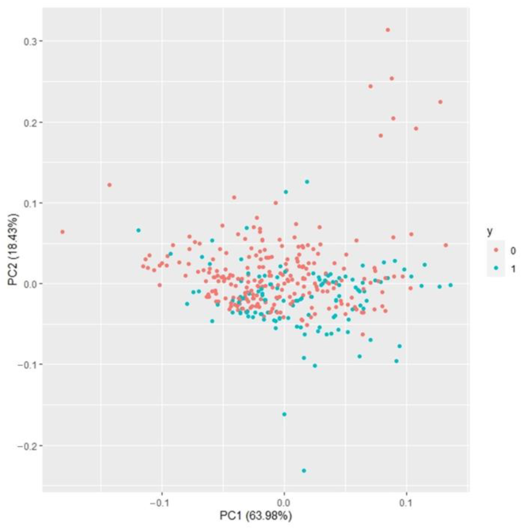When training a model using class-imbalanced data, the classification ability of the model tends to decline and involves a large bias, so the classification ability of the model for the minority classes can be poor [33,34,35]. In addition, several classes often share a common region in the data space, which is called class overlap [38], so they have similar feature values even though they belong to different classes, and this is a substantial obstacle in classification tasks. Consequently, the problems of collinearity, class imbalance, and class overlap must be considered when utilizing multiple SRI data to classify crop water status.

The difficulty of training models on collinear data can be overcome using machine learning, especially nonparametric methods [39]. Among the many nonparametric machine learning methods, random forest (RF) has a light computational burden [40] and can achieve excellent performance when the number of samples is small [41]. 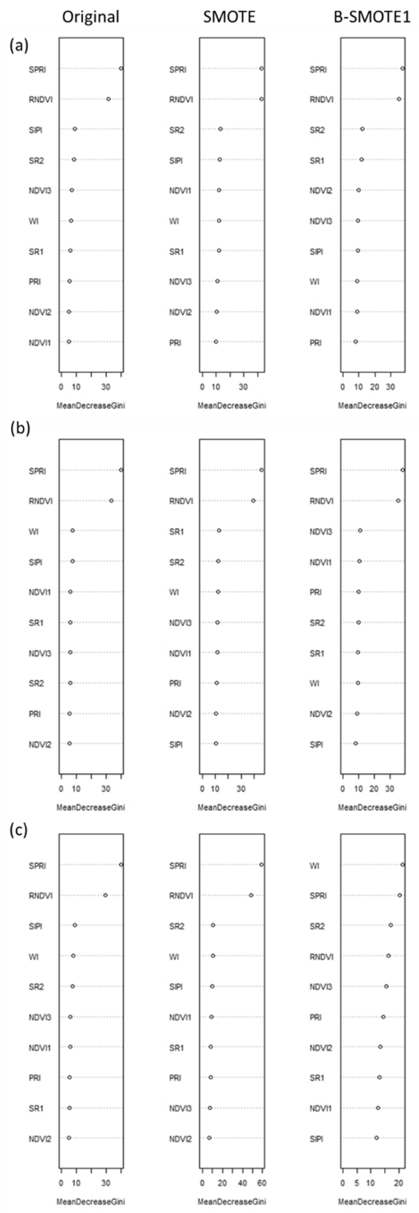In addition, RF is robust when extreme values or noise exist, and it is not prone to overfitting [40]. It can also assess the importance of each predictor, allowing researchers to further select important predictors to simplify the model [42]. There are two types of methods widely used to solve class imbalance and class overlap, namely, data-level and algorithm-level methods. The data-level methods are based on resampling the training dataset before the model training stage. The imbalanced data distribution can be adjusted or the boundaries strengthened between classes by oversampling the minority classes [35,38]. The algorithm-level methods involve proposing novel algorithms or modifying existing algorithms to directly handle datasets with class imbalance and overlap. However, algorithm-level methods require many technical thresholds in mathematics, statistics, and information engineering, so most studies focus on data-level methods that are simpler to implement [35].

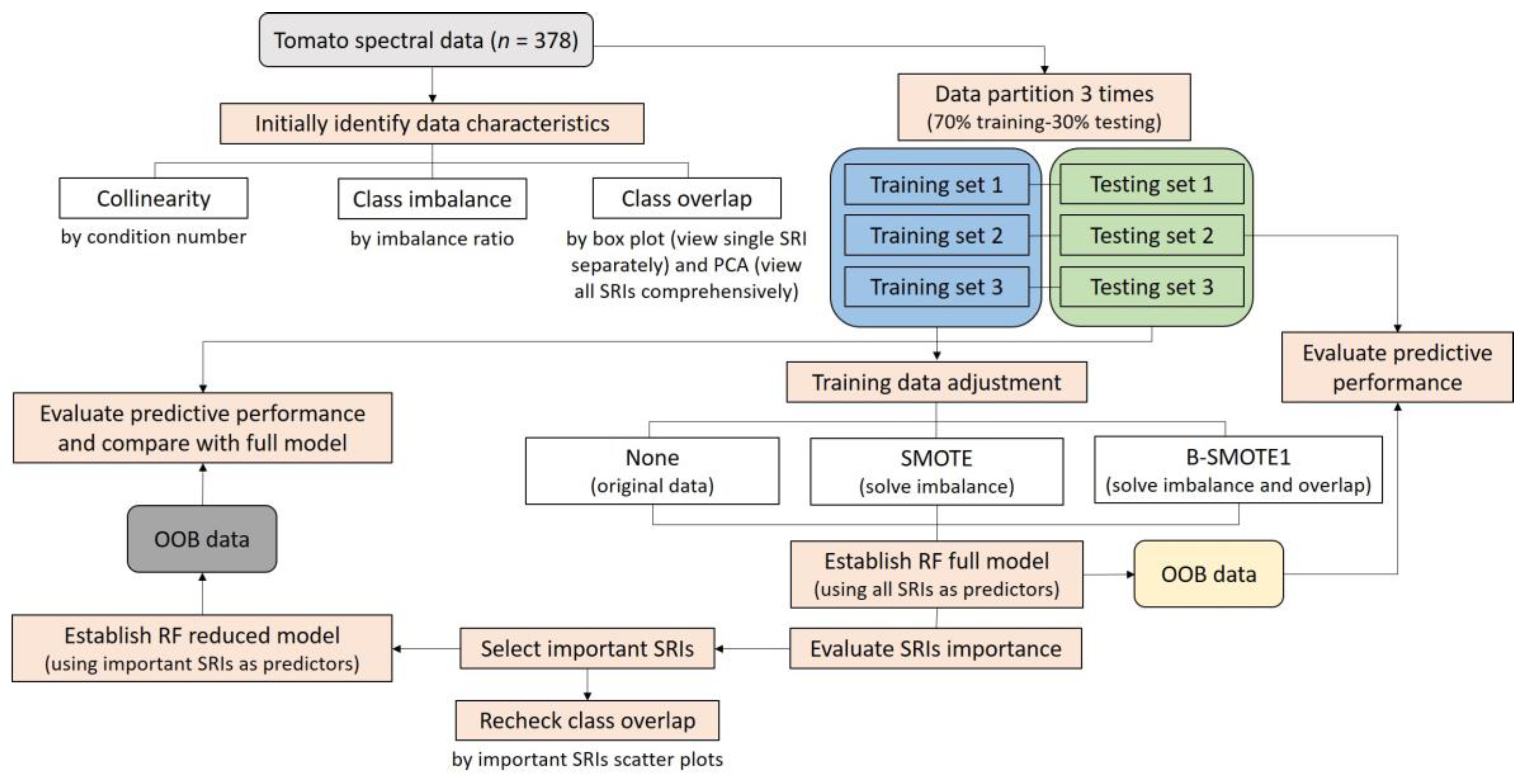
Available water resources are becoming more precious due to climate change and global warming. Agriculture, as an industry with a huge demand for water resources, must use water more precisely, reducing the amount of irrigation water without seriously negatively affecting the crop. This requires effective methods for detecting drought stress; therefore, this study combined SRIs, resampling techniques, and the RF algorithm to detect early drought stress in the vegetative stage of tomato. The study results are useful for the precise irrigation of greenhouse tomatoes and provide suggestions for spectral data analysis in detecting early drought stress.

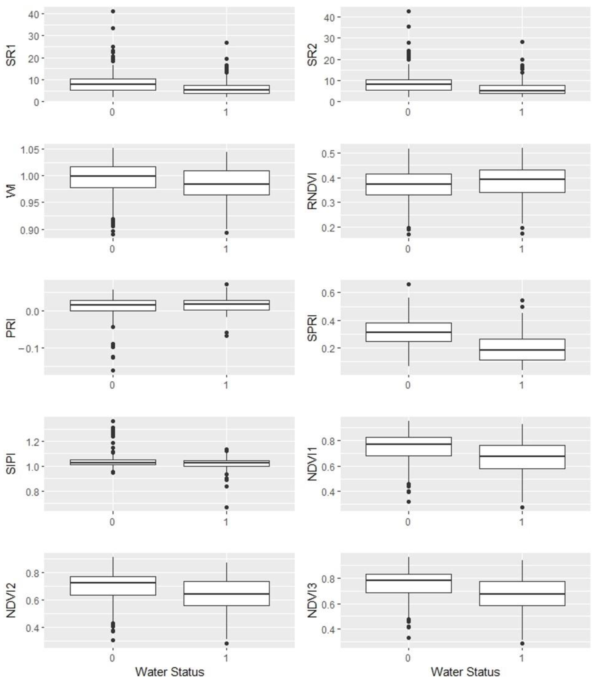
2. Materials and Methods

2.1. Data Source

The spectroscopic dataset on the tomato (cv. ‘Rosada’) vegetative stage was obtained from Tu et al. [23] and comprised 378 observations: 246 and 132 observations from ‘normal’ (coded as 0) and ‘water-deficit’ (coded as 1) tomatoes, respectively. Each observation in the dataset was recorded using an MS-720 Portable Spectroradiometer (EKO Instruments, San Jose, CA, USA) that detects the solar radiation reflecting from the canopy from 350 to 1050 nm and delivers data with a 3 nm interval. In that dataset, early drought stress was defined by the significantly decreased (p < 0.05) CO₂ assimilation rate, transpiration rate, and stomatal conductance of the tomato before the apparent water-deficit-related morphological alterations were observed. These key physiological parameters were collected using an LI-6800 Portable Photosynthesis System (LICOR Biosciences, Lincoln, NE, USA). This study used 14 in 211 wavebands for each spectral observation to calculate 10 SRIs (

Table 1. Constitution of spectral reflectance indices (SRIs) used for prediction model building.

Index Name	Acronym	Equation	Reference
Simple ratio 1	SR1	$\frac{{\mathrm{R}}_{800}}{{\mathrm{R}}_{680}}$	[43,44,45]
Simple ratio 2	SR2	$\frac{{\mathrm{R}}_{900}}{{\mathrm{R}}_{680}}$	[43,44,45]
Water index	WI	$\frac{{\mathrm{R}}_{900}}{{\mathrm{R}}_{970}}$	[43,46,47,48]
Normalized difference vegetation index 1	NDVI1	$\frac{{\mathrm{R}}_{800}-{\mathrm{R}}_{680}}{{\mathrm{R}}_{800}+{\mathrm{R}}_{680}}$	[43,45,47]
Normalized difference vegetation index 2	NDVI2	$\frac{{\mathrm{R}}_{800}-{\mathrm{R}}_{640}}{{\mathrm{R}}_{800}+{\mathrm{R}}_{640}}$	[49]
Normalized difference vegetation index 3	NDVI3	$\frac{{\mathrm{R}}_{860}-{\mathrm{R}}_{670}}{{\mathrm{R}}_{860}+{\mathrm{R}}_{670}}$	[50]
Red edge normalized difference vegetation index	RNDVI	$\frac{{\mathrm{R}}_{750}-{\mathrm{R}}_{705}}{{\mathrm{R}}_{750}+{\mathrm{R}}_{705}}$	[47,51]
Photochemical reflectance index	PRI	$\frac{{\mathrm{R}}_{531}-{\mathrm{R}}_{570}}{{\mathrm{R}}_{531}+{\mathrm{R}}_{570}}$	[47,48,49,52]
Similar photochemical reflectance index	SPRI	$\frac{{\mathrm{R}}_{560}-{\mathrm{R}}_{510}}{{\mathrm{R}}_{560}+{\mathrm{R}}_{510}}$	[53]
Structure-independent pigment index	SIPI	$\frac{{\mathrm{R}}_{800}-{\mathrm{R}}_{445}}{{\mathrm{R}}_{800}-{\mathrm{R}}_{680}}$	[48,49]

).

2.2. Identification of Collinearity, Class Imbalance, and Class Overlap

The condition number (κ) proposed by Belsley et al. [54] was used to assess the collinearity of the full set of predictors. If κ is large, very small differences in the predictor variables have huge influences on the regression coefficient estimation. Typically, a value of κ exceeding 15 indicates that harmful effects of collinearity can be present, so a correction is needed if the value of κ exceeds 30 [39]. The degree of class imbalance was measured as the imbalance ratio (IR), which was calculated as the number of the majority classes divided by the number of the minority classes. According to the IR value, the imbalance of a dataset can be defined as follows: balanced (1–1.5), slightly imbalanced (1.7–3.4), moderately imbalanced (8–16.4), and highly imbalanced (21.9 and above) [38]. There is no standard measurement of class overlap [38]; therefore, box plots, scatter plots, and principal component analysis (PCA) were used to present the class overlap of single, pairwise, and overall predictors. Box plots can graphically demonstrate the minimum, maximum, median, first quartile, third quartile, and outliers of a dataset. Scatter plots can directly present the distribution of data points in two or three dimensions. PCA is a popular multivariate method for reducing the dimensionality of a dataset while preserving the maximum amount of information and enabling the visualization of multidimensional data.

The statistical analyses were implemented using R software (version 4.1.3; R Foundation for Statistical Computing, Vienna, Austria). The ‘collin.fnc’ function in the ‘languageR’ package (version 1.5.0) was used to obtain the κ values. PCA was conducted using the ‘prcomp’ built-in function of R software.

2.3. Dataset Partition and Resampling Methods

In order to assess the performance and stability of the prediction model, the whole dataset was randomly divided into training and testing datasets at a ratio of 70:30 and repeated 3 times. Finally, 3 sets of training–testing data were generated. Training data were used to build a prediction model, while testing data did not participate in the model training and were just used to evaluate the accuracy of the prediction model in classifying new observations.

Table 2. Number of ‘normal’ and ‘water-deficit’ instances and the corresponding imbalance ratio (IR) of each training and testing dataset for building prediction models.

Set	Resampling Method	Training			Testing
		Normal	Water-Deficit	IR	Normal	Water-Deficit	IR
1	none	167	98	1.70	79	34	2.32
	SMOTE		196	1.17
	B-SMOTE1		137	1.22
2	none	168	97	1.73	78	35	2.23
	SMOTE		194	1.15
	B-SMOTE1		136	1.24
3	none	170	95	1.79	76	37	2.05
	SMOTE		190	1.12
	B-SMOTE1		145	1.17

SMOTE: synthetic minority over-sampling technique; B-SMOTE1: borderline-synthetic minority over-sampling technique 1.

displays the sample size for each training and testing set. Additionally, to solve class imbalance and class overlap, the synthetic minority over-sampling technique (SMOTE) [55] and its extension, borderline-SMOTE1 (B-SMOTE1) [56], were used to adjust the training data distribution. SMOTE generates synthetic samples through three steps: first, a minority observation $\overrightarrow{\mathrm{a}}$ is selected randomly; second, an observation $\overrightarrow{\mathrm{b}}$ among the K nearest neighbors of $\overrightarrow{\mathrm{a}}$ in the minority data is chosen at random; finally, these two observations are used to interpolate a new and nonrepeating minority sample $\overrightarrow{\mathrm{c}}$ (Equation (1)). SMOTE does not include any selection criteria for linear interpolation, whereas B-SMOTE1 tries to make synthetic samples generated near the decision boundary. For every instance in the minority class, B-SMOTE1 calculates C nearest neighbors, and the number of majority samples among the C nearest neighbors is denoted by C′. In B-SMOTE1, the number of majority neighbors of each minority instance is used to divide minority instances into three groups: SAFE (0 $\le$ C′ $<\frac{C}{2}$), DANGER ($\frac{C}{2}\le$ C′ $<$ C), and NOISE (C′ $=$ C), but only DANGER is used to generate synthetic instances in the B-SMOTE1 algorithm.

$$\overrightarrow{\mathrm{c}}=\overrightarrow{\mathrm{a}}+w(\overrightarrow{\mathrm{b}}-\overrightarrow{\mathrm{a}})$$

(1)

where w is a random weight with a value between 0 and 1.

In this study, the parameter K of SMOTE was set to 5, and the parameters C and K of B-SMOTE1 were set to 3 and 5, respectively. The data distribution adjusted by the resampling methods is shown in Table 2. Both the SMOTE and B-SMOTE1 were performed using the ‘smotefamily’ (version 1.3.1) package in the R software (version 4.1.3).

2.4. Establishment of Random Forest Model and Important Spectral Reflectance Indices Selection

RF is a nonparametric statistical method that does not require the assumptions of linear relationships and data distribution [57]. RF is formed by the aggregation of a large number of classification and regression trees (CARTs). Two hyperparameters are required before the RF training, ntree and mtry, where ntree is the number of CARTs grown in RF, and mtry is the number of candidate predictors when establishing the CARTs. Each CART is constructed from a bootstrap sample drawn with replacement from the training dataset, and the predictions of all CARTs are finally aggregated through the majority voting. In the RF algorithm, each CART uses the decrease of Gini impurity as a splitting criterion for generating nodes. Each time the CART in the RF splits a node, it randomly selects mtry candidate predictors, and the best splitting predictor is only determined among this randomly selected subset of predictors. RF can not only predict the response but also evaluate and rank predictors with respect to their contribution to predicting the response. The latter is automatically computed for each predictor within the RF algorithm. The importance of each predictor is measured as the mean decrease in Gini impurity (DGI). An important predictor is often selected for splitting and yields a high DGI. After the predictor importance is obtained and the predictors are sorted according to their importance, the important predictors can be determined according to the preset threshold [58].

In this study, ten SRIs were used as predictors of RF, and the screening criteria for important SRIs were set as the intersection of the top five important SRIs in the three training sets. After obtaining important SRIs, we used these SRIs to build the RF reduced model. The RF algorithm was implemented using the ‘randomForest’ package (version 4.6–14) in R software (version 4.1.3). For RF, ntree and mtry must be optimized to minimize the classification error. The optimal value of ntree was searched between 10 and 1000, and mtry was tuned using the ‘tuneRF’ function. The importance of each predictor, measured as the mean DGI, was calculated using the ‘importance’ function in the ‘randomForest’ package.

2.5. Model Performance Evaluation

Out-of-bag data (OOB data) or pre-split testing datasets can be used to evaluate the RF model performance [59]. The OOB data are those that have not been selected during the bootstrap sampling process. Moreover, each CART in the RF has its own OOB data. For the OOB data, each CART in RF is used to predict the respective OOB data and compare the predicted results with the actual results to evaluate the prediction performance. Another way to evaluate the prediction capacity is to preseparate a subset of the data as the testing data before training the RF, and then use the established model to make predictions on these testing data. Model performance was evaluated in terms of sensitivity (Sens), precision (Prec), F1 score (F1), accuracy (Acc), and balanced accuracy (bAcc), which are defined as follows:

$$Sens=\frac{\mathrm{T}\mathrm{P}}{\mathrm{T}\mathrm{P}+\mathrm{F}\mathrm{N}}\times 100\%$$

(2)

$$Prec=\frac{\mathrm{T}\mathrm{P}}{\mathrm{T}\mathrm{P}+\mathrm{F}\mathrm{P}}\times 100\%$$

(3)

$$F1=\frac{2\times \mathrm{S}\mathrm{e}\mathrm{n}\mathrm{s}\times \mathrm{P}\mathrm{r}\mathrm{e}\mathrm{c}}{\mathrm{S}\mathrm{e}\mathrm{n}\mathrm{s}+\mathrm{P}\mathrm{r}\mathrm{e}\mathrm{c}}$$

(4)

$$Acc=\frac{\mathrm{T}\mathrm{P}+\mathrm{T}\mathrm{N}}{\mathrm{T}\mathrm{P}+\mathrm{T}\mathrm{N}+\mathrm{F}\mathrm{P}+\mathrm{F}\mathrm{N}}\times 100\%$$

(5)

$$bAcc=\frac{\frac{\mathrm{T}\mathrm{P}}{\mathrm{T}\mathrm{P}+\mathrm{F}\mathrm{N}}+\frac{\mathrm{T}\mathrm{N}}{\mathrm{T}\mathrm{N}+\mathrm{F}\mathrm{P}}}{2}\times 100\%$$

(6)

where TN is the number of true negatives (when the actual water status of the tomato was ‘normal’, and the model also classified it as ‘normal’); FP is the number of false positives (when the actual water status of the tomato was ‘normal’ but the model classified it as ‘water-deficit’); FN is the number of false negatives (when the actual water status of the tomato was ‘water-deficit’ but the model classified it as ‘normal’); and TP is the number of true positives (when the actual water status of the tomato was ‘water-deficit’ and the model also classified it as ‘water-deficit’). The range of these metrics is between 0–100%; the closer to 100%, the better the model performance.

3. Results and Discussion

The study workflow is illustrated in Figure 1. Briefly, possible problems for the spectral data were identified, such as collinearity, class imbalance, and class overlap. Then, three training/testing datasets were generated and adjusted using three resampling methods, namely, nonresampling (original data), SMOTE, and B-SMOTE1, respectively. The third step was to build the RF full model with the ten SRIs and evaluate the importance of each SRI. After selecting the important SRIs, the RF reduced model was built with fewer predictors, and the class overlap was reexamined. Finally, the three resampling methods and the predictive performance of the full and reduced models were compared.

3.1. Diagnosis of Data Problems

The predictors used in this study to establish an early drought stress detection model were ten SRIs (composed of 14 wavebands), and the response variable was the tomato water status, i.e., ‘normal’ or ‘water-deficit’. Regarding collinearity, κ = 757.595, which means the data were highly collinear (κ > 30). If a dataset is characterized by substantial collinearity, at least two problems may arise when using the parametric method. First, parameter estimates may assume counterintuitive and theoretically uninterpretable values. Second, no predictor may be statistically significant in explaining the variation of the response [60]. In order to demonstrate the difficulty of parametric methods in dealing with highly collinear data, we used a popular classification method, namely, logistic regression, to build prediction models. Logistic regression is similar to linear regression, except that its dependent variable is binary (e.g., normal/water-deficit) rather than continuous. The positive and negative signs of the parameter estimate for logistic regression reflect the relationship between the SRI value and the water status. A positive sign means that the larger the SRI value, the more likely it was a ‘water-deficit’ sample; conversely, a negative sign indicates that the smaller the SRI value, the more likely it was a ‘water-deficit’ sample. It was found that when the ten SRIs were used as independent variables simultaneously, the coefficient estimates of each SRI calculated by logistic regression were very different among three sets, and even the positive and negative signs were inconsistent (

Table 3. Parameter estimates for each SRI of logistic regression were established with three original training datasets. A positive sign means that the larger the SRI value, the more likely it was a ‘water-deficit’ sample; conversely, a negative sign means that the smaller the SRI value, the more likely it was a ‘water-deficit’ sample.

Set	Spectral Reflectance Indices
	SR1	SR2	WI	RNDVI	PRI	SPRI	SIPI	NDVI1	NDVI2	NDVI3
1	0.80	$-$0.73	$-$48.40	96.07	9.01	$-$11.12	12.33	13.22	26.08	$-$80.43
2	0.25	0.02	$-$36.38	102.10	$-$4.86	$-$23.94	10.58	34.50	$-$9.08	$-$68.71
3	$-$0.65	0.53	$-$35.89	110.63	0.31	$-$6.47	1.18	2.91	33.35	$-$85.98

). This result reflected the instability caused by collinearity in parameter estimation using parametric methods.

A common strategy for resolving the problem of collinearity for spectral data is to implement the partial least squares model, but a suitable preprocessing method for the spectral data usually has to be chosen [61]. In contrast, machine learning methods (e.g., RF) put more emphasis on achieving efficient extraction of important features and accurate prediction of response, so the complex task of spectral preprocessing can be avoided [27].

The study dataset comprised 246 ‘normal’ and 132 ‘water-deficit’ observations, and the IR was 1.86, indicating that the data were slightly imbalanced. After three random samplings, the IR of the original training datasets was between 1.70 and 1.79, and the IR of the testing datasets ranged from 2.05 to 2.32 (Table 2). In the case of class imbalance, it is difficult for the classification model to determine the correct classification rules due to the scarcity of minority class data in the training set [36]. In addition, the class imbalance is often accompanied by class overlap [35]. It can be observed from the respective box plots of the SRIs used as predictors that only the distribution of SPRI was different between the two water statuses, with considerable overlap between the other SRIs (Figure 2). Since ten SRIs were used as predictors, which cannot be presented in a scatter plot, PCA was applied to comprehensively investigate the class overlap of all predictors. It was found that projecting the data of the ten SRIs from a high dimension to a two-dimensional plane retained more than 80% of the data variation (Figure 3). It can be seen from the PCA score plot that the sample distributions of the two water statuses had a high overlap.

In summary, the study data suffered from the problems of collinearity, class imbalance, and class overlap; therefore, the RF algorithm less affected by collinearity was employed in model training to establish the prediction model, and SMOTE and B-SMOTE1 were used to adjust the original training datasets to reduce the IR values (Table 2).

3.2. Evaluation of RF Full Model’s Predictive Performance and Predictors’ Importance

The optimal hyperparameter values of the RF full model built using ten SRIs as predictors and the prediction results for the OOB data and testing dataset are shown in Table S1, with the average and standard deviation of the model performance metrics established by the same resampling method in the three datasets shown in

Table 4. The performance of the RF full models built using three resampling methods to predict OOB data and testing data. The performance metrics are presented as the mean ± standard deviation. The range of these metrics is between 0–100%; the closer to 100%, the better the model performance.

Resampling Method	Data	Performance Metrics
		Sens	Prec	F1	Acc	bAcc
Nonresampling	OOB	81.0% $\pm$ 3.0%	86.4% $\pm$ 0.8%	83.6% $\pm$ 1.5%	88.4% $\pm$ 0.8%	86.8% $\pm$ 1.2%
	testing	79.2% $\pm$ 7.6%	82.4% $\pm$ 1.3%	80.5% $\pm$ 3.9%	88.2% $\pm$ 1.7%	85.7% $\pm$ 3.3%
SMOTE	OOB	91.4% $\pm$ 1.8%	91.9% $\pm$ 0.7%	91.6% $\pm$ 0.9%	91.1% $\pm$ 0.9%	91.0% $\pm$ 0.8%
	testing	83.0% $\pm$ 6.2%	78.2% $\pm$ 4.8%	80.3% $\pm$ 2.8%	87.3% $\pm$ 1.5%	86.2% $\pm$ 2.2%
B-SMOTE1	OOB	83.8% $\pm$ 7.3%	86.7% $\pm$ 7.7%	85.2% $\pm$ 7.4%	86.8% $\pm$ 6.9%	86.5% $\pm$ 6.9%
	testing	79.0% $\pm$ 8.1%	81.7% $\pm$ 6.8%	80.2% $\pm$ 6.9%	85.9% $\pm$ 5.1%	84.7% $\pm$ 5.6%

OOB data: out-of-bag data; Sens: sensitivity; Prec: precision; F1: F1 score; Acc: accuracy; bAcc: balanced accuracy.

. The RF full model established by the original data achieved Sens of 79.2%, Prec of 82.4%, F1 of 80.3%, and Acc of 88.2% when predicting the testing data. This performance is better than the RF models in previous works [23,27], which used the same training data. It is worth noting that all 211 spectral wavebands were used as predictors of RF in the previous studies, whereas the model with 10 SRIs (composed of only 14 wavebands) could achieve a better performance in this study. This also reflects that the SRI is a more appropriate predictor than separate spectral wavebands.

According to the results of this study, adjusting the training data distribution through SMOTE greatly improved the performance of predicting OOB data, especially Sens; however, the value of Prec slightly decreased when employing this model to predict the testing data. The RF full model trained with SMOTE had a higher Sens and lower Prec, indicating fewer false negative cases (where the actual water status of the tomato is ‘water-deficit’, but the model classifies it as ‘normal’) and more false positive cases (where the actual water status of the tomato is ‘normal’, but the model classifies it as ‘water-deficit’). In general, the choice of suitable models depends on different misclassification costs and user’s objectives or demands. Regarding the capability of evaluating model classification, F1, Acc, and bAcc are more comprehensive metrics than Sens and Prec [62]. Moreover, when the data suffer from class imbalance, bAcc is one of the most reliable metrics [38]. From the perspective of bAcc, the model built with SMOTE performed the best (Table 4). Notably, although the data used seemed to have class overlap (Figure 2 and Figure 3), the model established by B-SMOTE1 utilized to resolve this problem was not much improved (Table 4); rather, it performed worse in predicting the testing data. Unfortunately, adjustments to the training data do not always bring a positive effect.

Among the nine combinations (3 datasets × 3 resampling methods) performed in this study, two SRIs, namely, SPRI and RNDVI, were prominent with mean DGIs almost three times higher than those of the other SRIs (Figure 4). The top five important SRIs are summarized in

Table 5. The top five important SRIs selected by RF models using the mean decrease in Gini impurity.

Data	Set	Important Reflectance Spectral Indices
Original	1	SPRI, RNDVI, SIPI, SR2, NDVI3
	2	SPRI, RNDVI, WI, SIPI, NDVI1
	3	SPRI, RNDVI, SIPI, WI, SR2
SMOTE	1	SPRI, RNDVI, SR2, SIPI, NDVI1
	2	SPRI, RNDVI, SR1, SR2, WI
	3	SPRI, RNDVI, SR2, WI, SIPI
B-SMOTE1	1	SPRI, RNDVI, SR2, SR1, NDVI2
	2	SPRI, RNDVI, NDVI3, NDVI1, PRI
	3	WI, SPRI, SR2, RNDVI, NDVI3

. Regardless of the resampling technique used, RNDVI and SPRI were important predictors. In addition, SR2 was one of the top five important predictors in the three SMOTE-processed datasets. This SRI also appeared twice in the top five lists of the three sets for original and B-SMOTE1 processed data. RNDVI, SPRI, and SR2 have been studied in dwarf green beans (Phaseolus vulgaris humilis) [44], sugar beet (Beta vulgaris) [45], tomato [47], olive (Olea europaea) [51], and rocket (Eruca sativa) [53] and have been proven to be useful in assessing the plant water status in open fields or greenhouses. Therefore, only these three SRIs were used in the next step to build the reduced models.

3.3. Predictive Performance of Reduced Models and Model Comparison

The optimal hyperparameter values of the RF reduced model built using SPRI, RNDVI, and SR2 and the prediction results for the OOB data and testing dataset are shown in Table S1 with the average and standard deviation of the model performance metrics shown in

Table 6. The performance of the RF reduced models built using three resampling methods to predict OOB data and testing data. The performance metrics are presented as the mean ± standard deviation. The range of these metrics is between 0–100%; the closer to 100%, the better the model performance.

Resampling Method	Data	Performance Metrics
		Sens	Prec	F1	Acc	bAcc
Nonresampling	OOB	87.2% $\pm$ 2.0%	77.6% $\pm$ 1.3%	82.1% $\pm$ 1.6%	87.7% $\pm$ 0.9%	87.5% $\pm$ 1.2%
	testing	77.3% $\pm$ 6.4%	83.2% $\pm$ 8.9%	79.5% $\pm$ 4.1%	87.6% $\pm$ 2.6%	84.8% $\pm$ 2.7%
SMOTE	OOB	91.6% $\pm$ 1.4%	90.3% $\pm$ 1.4%	91.0% $\pm$ 1.4%	90.4% $\pm$ 1.4%	90.3% $\pm$ 1.4%
	testing	83.0% $\pm$ 6.2%	76.7% $\pm$ 7.1%	79.3% $\pm$ 3.6%	86.4% $\pm$ 2.5%	85.5% $\pm$ 2.3%
B-SMOTE1	OOB	83.4% $\pm$ 11.2%	83.0% $\pm$ 10.0%	83.1% $\pm$ 10.5%	84.9% $\pm$ 9.7%	84.8% $\pm$ 9.8%
	testing	79.8% $\pm$ 10.8%	80.1% $\pm$ 9.6%	79.8% $\pm$ 9.6%	85.6% $\pm$ 6.9%	84.5% $\pm$ 7.7%

. The model trained by adjusting the training data distribution with SMOTE had the highest Sens and bAcc, while the model trained by B-SMOTE1 performed the worst. The class overlap was reexamined to determine the reason for the poor B-SMOTE1 performance. Since there were only three SRIs, pairwise and three-dimensional scatter plots were plotted. Scatter plots showed that the overlapping was almost nonexistent, so the water status data points were well separated in two or three dimensions (Figure 5), whereas there were some synthetic ‘water-deficit’ samples (green points) surrounded mainly by the ‘normal’ samples (red points) in the scatter plots of the B-SMOTE1 processed data (Figure 6). Thus, we speculate that when the class imbalance and class overlap are not severe, the property of B-SMOTE1 that limits the synthetic samples generated at decision boundaries may increase the complexity of the data, thereby causing difficulties in model classification. This result may also explain the poor performance of B-SMOTE1 in the RF full model (Table 4). Since there is no standard method for detecting the class overlap, especially in high-dimensional situations [38], the box plot (Figure 2) and PCA (Figure 3) used in this study may not truly represent the distribution of data points in the high dimension, which leads to a bias in judging class overlap. Based on these results, we suggest that before applying B-SMOTE1 on high-dimensional data, researchers can first screen out two to three important predictors and then use a scatter plot to detect the class overlap. We propose that screening important predictors can simplify the model to reduce data collection costs and help researchers see the characteristics of the data more easily and choose appropriate analysis methods.

Finally, the performance of the full model (using all ten SRIs) and the reduced model (using only RNDVI, SPRI, and SR2) trained by adjusting the training data distribution with SMOTE were compared, showing that the reduced model metrics, except the value of Sens, were about 1% lower than those of the full model (Table 4 and Table 6). Even though the performance of the reduced model decreased, it still had Sens of 83.0–91.6%, Prec of 76.7–90.3%, F1 of 79.3–91.0%, Acc of 86.4–90.4%, and bAcc of 85.5–90.3%. More importantly, the number of spectral wavebands reduced from 14 to 6, i.e., 510, 560, 680, 705, 750, and 900 nm, achieving the benefits of reducing data collection costs and computational loading. There are many machine learning methods that are more powerful than RF and can handle spectral data well. For example, Tu et al. [23] proposed a convolutional neural network (CNN), 1D-SP-Net, to deal with the imbalanced data. Kuo et al. [27] established a CNN, 1D-ResGC-Net, for feature selection in spectral data. However, the training requirements of these methods are much more complex than those of RF. The RF combined with the SMOTE method in this study makes it easier to build a model and can achieve performance comparable to CNN. In summary, the proposed RF model can accurately detect early drought stress in the vegetative stage of greenhouse tomatoes using three SRIs, namely, RNDVI, SPRI, and SR2, to provide a useful auxiliary tool for precise irrigation. In the future, a sensor prototype can be developed based on the results of this study and tested on different tomato varieties and growth stages. Tomato yield and fruit quality should also be included in the assessment. These efforts can make the tool more comprehensive and reliable.

4. Conclusions

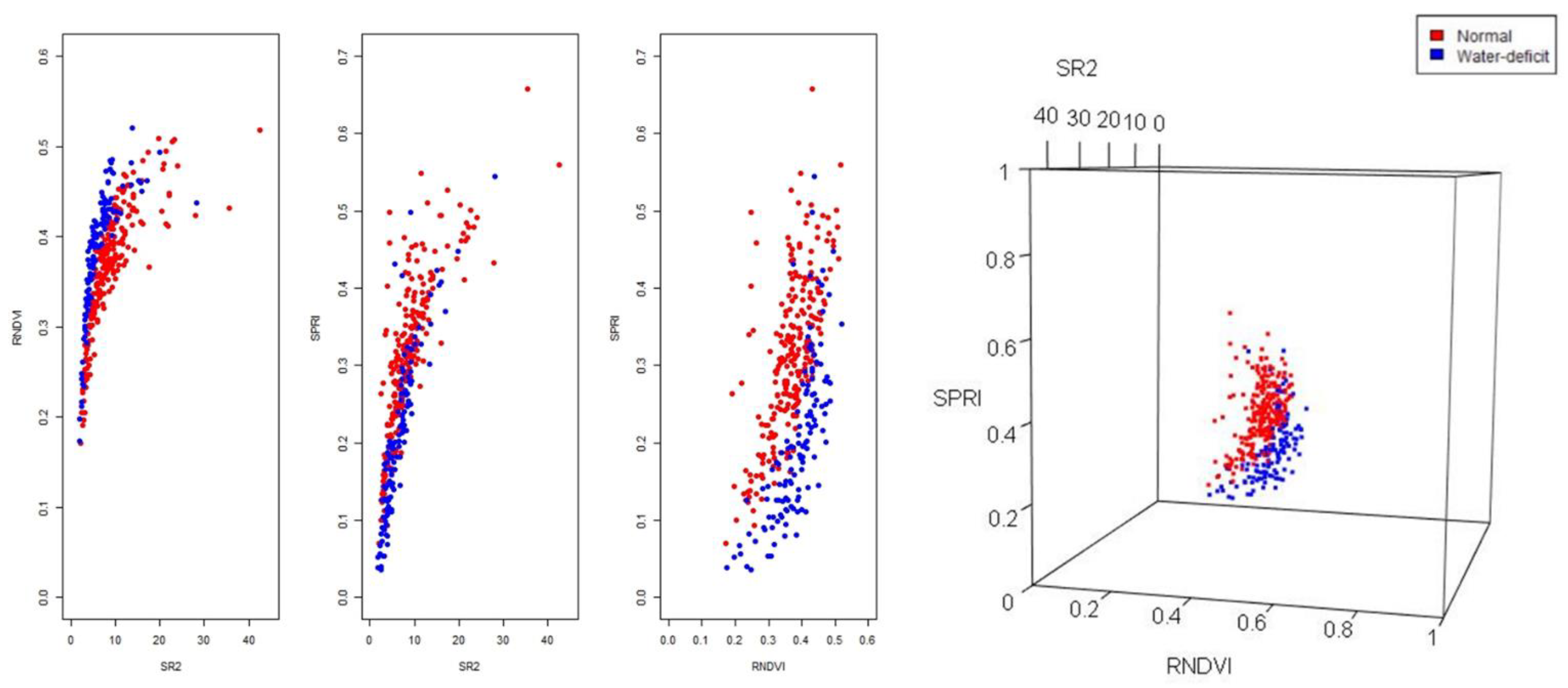
Real-time detection of plant drought stress through noncontact and nondestructive sensors to meet the water needs of greenhouse crop production is one of the directions of precision irrigation. Many SRIs have been proposed to establish the prediction model, but the spectral data often suffer from problems of collinearity, class imbalance, and class overlap, which require some effective strategies to overcome. This study developed an early drought detection model for the vegetative stage of greenhouse tomatoes and explored the strategies for analyzing multiple SRI data. It was found that using RF to build the model can overcome collinearity well. For class imbalance, SMOTE can be used to adjust the training data distribution to improve the model’s ability to identify minority classes. For the class overlap in high-dimensional data, we suggest that researchers can first screen out two to three important predictors and then use scatter plots to detect the class overlap. When there is indeed class overlap in the data, resampling techniques developed to address class overlap (e.g., B-SMOTE1) can be used to process the training data. Finally, the proposed RF model for detecting early drought stress based on three SRIs, namely, SPRI, RNDVI, and SR2, which only require six spectral wavebands, i.e., 510, 560, 680, 705, 750, and 900 nm, achieved more than 85% accuracy. We concluded that this reduced model can serve as a useful and cost-effective tool for precise irrigation in greenhouse tomato production. A sensor prototype can be developed and tested in different situations to make it more comprehensive and reliable.

References

1. FAO. FAOSTAT. 2023. Available online: https://www.fao.org/faostat/en/#data (accessed on 25 November 2023).
2. IPCC. Managing the risks of extreme events and disasters to advance climate change adaptation. In A Special Report of Working Groups I and II of the Intergovernmental Panel on Climate Change; Field, C.B., Barros, V., Stocker, T.F., Qin, D., Dokken, D.J., Ebi, K.L., Eds.; IPCC: Geneva, Switzerland, 2012. [Google Scholar]
3. Cogato, A.; Meggio, F.; De Antoni Migliorati, M.; Marinello, F. Extreme weather events in agriculture: A systematic review. Sustainability 2019, 11, 2547. [Google Scholar] [CrossRef]
4. Mankin, J.S.; Seager, R.; Smerdon, J.E.; Cook, B.I.; Williams, A.P. Mid-latitude freshwater availability reduced by projected vegetation responses to climate change. Nat. Geosci. 2019, 12, 983–988. [Google Scholar] [CrossRef]
5. Pokhrel, Y.; Felfelani, F.; Satoh, Y.; Boulange, J.; Burek, P.; Gädeke, A.; Gerten, D.; Gosling, S.N.; Grillakis, M.; Gudmundsson, L.; et al. Global terrestrial water storage and drought severity under climate change. Nat. Clim. Change 2021, 11, 226–233. [Google Scholar] [CrossRef]
6. Boyer, J.S. Plant productivity and environment. Science 1982, 218, 443–448. [Google Scholar] [CrossRef] [PubMed]
7. Calzadilla, A.; Rehdanz, K.; Tol, R.S.J. Water scarcity and the impact of improved irrigation management: A computable general equilibrium analysis. Agric. Econ. 2011, 42, 305–323. [Google Scholar] [CrossRef]
8. Huang, K.-M.; Guan, Z.; Hammami, A. The US fresh fruit and vegetable industry: An overview of production and trade. Agriculture 2022, 12, 1719. [Google Scholar] [CrossRef]
9. Domingo, R.; Pérez-Pastor, A.; Ruiz-Sánchez, M.C. Physiological responses of apricot plants grafted on two different rootstocks to flooding conditions. J. Plant Physiol. 2002, 159, 725–732. [Google Scholar] [CrossRef]
10. Shao, G.; Huang, D.; Cheng, X.; Cui, J.; Zhang, Z. Path analysis of sap flow of tomato under rain shelters in response to drought stress. Int. J. Agric. Biol. Eng. 2016, 9, 54–62. [Google Scholar] [CrossRef]
11. Jangid, K.K.; Dwivedi, P. Physiological responses of drought stress in tomato: A review. Int. J. Environ. Agric. Biotech. 2016, 9, 53. [Google Scholar] [CrossRef]
12. Nangare, D.D.; Singh, Y.; Kumar, P.S.; Minhas, P.S. Growth, fruit yield and quality of tomato (Lycopersicon esculentum Mill.) as affected by deficit irrigation regulated on phenological basis. Agric. Water Manag. 2016, 171, 73–79. [Google Scholar] [CrossRef]
13. Buttaro, D.; Santamaria, P.; Signore, A.; Cantore, V.; Boari, F.; Montesano, F.F.; Parente, A. Irrigation management of greenhouse tomato and cucumber using tensiometer: Effects on yield, quality and water use. Agric. Agric. Sci. Procedia 2015, 4, 440–444. [Google Scholar] [CrossRef]
14. Cui, J.; Shao, G.; Lu, J.; Keabetswe, L.; Hoogenboom, G. Yield, quality and drought sensitivity of tomato to water deficit during different growth stages. Sci. Agric. 2019, 77, e20180390. [Google Scholar] [CrossRef]
15. Wu, Y.; Yan, S.; Fan, J.; Zhang, F.; Xiang, Y.; Zheng, J.; Guo, J. Responses of growth, fruit yield, quality and water productivity of greenhouse tomato to deficit drip irrigation. Sci. Hortic. 2021, 275, 109710. [Google Scholar] [CrossRef]
16. Li, H.; Guo, Y.; Zhao, H.; Wang, Y.; Chow, D. Towards automated greenhouse: A state of the art review on greenhouse monitoring methods and technologies based on the internet of things. Comput. Electron. Agric. 2021, 191, 106558. [Google Scholar] [CrossRef]
17. Fang, S.-L.; Chang, T.-J.; Tu, Y.-K.; Chen, H.-W.; Yao, M.-H.; Kuo, B.-J. Plant-response-based control strategy for irrigation and environmental controls for greenhouse tomato seedling cultivation. Agriculture 2022, 12, 633. [Google Scholar] [CrossRef]
18. Fang, S.-L.; Tu, Y.-K.; Kang, L.; Chen, H.-W.; Chang, T.-J.; Yao, M.-H.; Kuo, B.-J. CART model to classify the drought status of diverse tomato genotypes by VPD, air temperature, and leaf–air temperature difference. Sci. Rep. 2023, 13, 602. [Google Scholar] [CrossRef]
19. Kacira, M.; Sase, S.; Okushima, L.; Ling, P.P. Plant response-based sensing for control strategies in sustainable greenhouse production. J. Agric. Meteorol. 2005, 61, 15–22. [Google Scholar] [CrossRef]
20. Lichtenthaler, H.K. The stress concept in plants: An introduction. Ann. N. Y. Acad. Sci. 1998, 851, 187–198. [Google Scholar] [CrossRef]
21. Katsoulas, N.; Elvanidi, A.; Ferentinos, K.P.; Kacira, M.; Bartzanas, T.; Kittas, C. Crop reflectance monitoring as a tool for water stress detection in greenhouses: A review. Biosyst. Eng. 2016, 151, 374–398. [Google Scholar] [CrossRef]
22. Behmann, J.; Steinrücken, J.; Plümer, L. Detection of early plant stress responses in hyperspectral images. ISPRS J. Photogramm. Remote Sens. 2014, 93, 98–111. [Google Scholar] [CrossRef]
23. Tu, Y.-K.; Kuo, C.-E.; Fang, S.-L.; Chen, H.-W.; Chi, M.-K.; Yao, M.-H.; Kuo, B.-J. A 1D-SP-Net to determine early drought stress status of tomato (Solanum lycopersicum) with imbalanced Vis/NIR spectroscopy data. Agriculture 2022, 12, 259. [Google Scholar] [CrossRef]
24. Fernández-Novales, J.; Tardaguila, J.; Gutiérrez, S.; Marañón, M.; Diago, M.P. In-field quantification and discrimination of different vineyard water regimes by on-the-go NIR spectroscopy. Biosyst. Eng. 2018, 165, 47–58. [Google Scholar] [CrossRef]
25. Carter, G.A. Primary and secondary effects of water content on the spectral reflectance of leaves. Am. J. Bot. 1991, 78, 916–924. [Google Scholar] [CrossRef]
26. Elvanidi, A.; Katsoulas, N.; Ferentinos, K.P.; Bartzanas, T.; Kittas, C. Hyperspectral machine vision as a tool for water stress severity assessment in soilless tomato crop. Biosyst. Eng. 2018, 165, 25–35. [Google Scholar] [CrossRef]
27. Kuo, C.-E.; Tu, Y.-K.; Fang, S.-L.; Huang, Y.-R.; Chen, H.-W.; Yao, M.-H.; Kuo, B.-J. Early detection of drought stress in tomato from spectroscopic data: A novel convolutional neural network with feature selection. Chemometr. Intell. Lab. Syst. 2023, 239, 104869. [Google Scholar] [CrossRef]
28. Sims, D.A.; Gamon, J.A. Relationships between leaf pigment content and spectral reflectance across a wide range of species, leaf structures, and developmental stages. Remote Sens. Environ. 2002, 81, 337–354. [Google Scholar] [CrossRef]
29. Thenkabail, P.S.; Smith, R.B.; De Pauw, E. Hyperspectral vegetation indices and their relationships with agricultural crop characteristics. Remote Sens. Environ. 2000, 71, 158–182. [Google Scholar] [CrossRef]
30. Rosa, A.P.; Barão, L.; Chambel, L.; Cruz, C.; Santana, M.M. Early identification of plant drought stress responses: Changes in leaf reflectance and plant growth promoting rhizobacteria selection-the case study of tomato plants. Agronomy 2023, 13, 183. [Google Scholar] [CrossRef]
31. Mariotto, I.; Thenkabail, P.S.; Huete, A.; Slonecker, E.T.; Platonov, A. Hyperspectral vs. multispectral crop-productivity modeling and type discrimination for the HyspIRI mission. Remote Sens. Environ. 2013, 139, 291–305. [Google Scholar] [CrossRef]
32. Yi, Q.; Jiapaer, G.; Chen, J.; Bao, A.; Wang, F. Different units of measurement of carotenoids estimation in cotton using hyperspectral indices and partial least squares regression. ISPRS J. Photogramm. Remote Sens. 2014, 91, 72–84. [Google Scholar] [CrossRef]
33. Ali, H.; Salleh, M.N.M.; Saedudin, R.; Hussain, K.; Mushtaq, M.F. Imbalance class problems in data mining: A review. Indones. J. Electr. Eng. Comput. Sci. 2019, 14, 1560–1571. [Google Scholar] [CrossRef]
34. Douzas, G.; Bacao, F.; Last, F. Improving imbalanced learning through a heuristic oversampling method based on k-means and SMOTE. Inf. Sci. 2018, 465, 1–20. [Google Scholar] [CrossRef]
35. Lin, W.-C.; Tsai, C.-F.; Hu, Y.-H.; Jhang, J.-S. Clustering-based undersampling in class-imbalanced data. Inf. Sci. 2017, 409–410, 17–26. [Google Scholar] [CrossRef]
36. Ali, A.; Shamsuddin, S.M.; Ralescu, A.L. Classification with the class imbalance problem: A review. Int. J. Advance Soft Compu. Appl. 2013, 5, 1–31. [Google Scholar]
37. Garcia, V.; Sanchez, J.S.; Mollineda, R.A. On the effectiveness of preprocessing methods when dealing with different levels of class imbalance. Knowl. Based Syst. 2012, 25, 13–21. [Google Scholar] [CrossRef]
38. Vuttipittayamongkol, P.; Elyan, E.; Petrovski, A. On the class overlap problem in imbalanced data classification. Knowl. Based Syst. 2021, 212, 106631. [Google Scholar] [CrossRef]
39. Tomaschek, F.; Hendrix, P.; Baayen, R.H. Strategies for addressing collinearity in multivariate linguistic data. J. Phon. 2018, 71, 249–267. [Google Scholar] [CrossRef]
40. Rodriguez-Galiano, V.F.; Ghimire, B.; Rogan, J.; Chica-Olmo, M.; Rigol-Sanchez, J.P. An assessment of the effectiveness of a random forest classifier for land-cover classification. ISPRS J. Photogramm. Remote Sens. 2012, 67, 93–104. [Google Scholar] [CrossRef]
41. Boulesteix, A.-L.; Janitza, S.; Kruppa, J.; König, I.R. Overview of random forest methodology and practical guidance with emphasis on computational biology and bioinformatics. Wiley Interdiscip. Rev. Data Min. Knowl. Discov. 2012, 2, 493–507. [Google Scholar] [CrossRef]
42. Speiser, J.L.; Miller, M.E.; Tooze, J.; Ip, E. A comparison of random forest variable selection methods for classification prediction modeling. Expert Syst. Appl. 2019, 134, 93–101. [Google Scholar] [CrossRef]
43. Genc, L.; Demirel, K.; Camoglu, G.; Asik, S.; Smith, S. Determination of plant water stress using spectral reflectance measurements in watermelon (Citrullus vulgaris). Am.-Eurasian J. Agric. Environ. Sci. 2011, 11, 296–304. [Google Scholar]
44. Köksal, E.S. Hyperspectral reflectance data processing through cluster and principal component analysis for estimating irrigation and yield related indicators. Agric. Water Manag. 2011, 98, 1317–1328. [Google Scholar] [CrossRef]
45. Köksal, E.S.; Güngör, Y.; Yildirim, Y.E. Spectral reflectance characteristics of sugar beet under different levels of irrigation water and relationships between growth parameters and spectral indexes. Irrig. Drain. 2010, 60, 187–195. [Google Scholar] [CrossRef]
46. Clevers, J.G.P.W.; Kooistra, L.; Schaepman, M.E. Using spectral information from the NIR water absorption features for the retrieval of canopy water content. Int. J. Appl. Earth Obs. Geoinf. 2008, 10, 388–397. [Google Scholar] [CrossRef]
47. Kittas, C.; Elvanidi, A.; Katsoulas, N.; Ferentinos, K.P.; Bartzanas, T. Reflectance indices for the detection of water stress in greenhouse tomato (Solanum lycopersicum). Acta Hortic. 2016, 1112, 63–70. [Google Scholar] [CrossRef]
48. Sun, P.; Grignetti, A.; Liu, S.; Casacchia, R.; Salvatori, R.; Pietrini, F.; Loreto, F.; Centritto, M. Associated changes in physiological parameters and spectral reflectance indices in olive (Olea europaea L.) leaves in response to different levels of water stress. Int. J. Remote Sens. 2008, 29, 1725–1743. [Google Scholar] [CrossRef]
49. Jones, C.L.; Weckler, P.R.; Maness, N.O.; Stone, M.L.; Jayasekara, R. Estimating water stress in plants using hyperspectral sensing. In Proceedings of the 2004 ASAE Annual Meeting, Ottawa, ON, Canada, 1–4 August 2004; p. 1. [Google Scholar] [CrossRef]
50. Borzuchowski, J.; Schulz, K. Retrieval of leaf area index (LAI) and soil water content (WC) using hyperspectral remote sensing under controlled glasshouse conditions for spring barley and sugar beet. Remote Sens. 2010, 2, 1702–1721. [Google Scholar] [CrossRef]
51. Marino, G.; Pallozzi, E.; Cocozza, C.; Tognetti, R.; Giovannelli, A.; Cantini, C.; Centritto, M. Assessing gas exchange, sap flow and water relations using tree canopy spectral reflectance indices in irrigated and rainfed Olea europaea L. Environ. Exp. Bot. 2014, 99, 43–52. [Google Scholar] [CrossRef]
52. Sarlikioti, V.; Driever, S.M.; Marcelis, L.F.M. Photochemical reflectance index as a mean of monitoring early water stress. Ann. Appl. Biol. 2010, 157, 81–89. [Google Scholar] [CrossRef]
53. Tsirogiannis, I.L.; Katsoulas, N.; Savvas, D.; Karras, G.; Kittas, C. Relationships between reflectance and water status in a greenhouse rocket (Eruca sativa Mill.) cultivation. Europ. J. Hort. Sci. 2013, 78, 275–282. [Google Scholar]
54. Belsley, D.A.; Kuh, E.; Welsch, R.E. Regression Diagnostics: Identifying Influential Data and Sources of Collinearity; John Wiley & Sons, Inc.: New York, NY, USA, 1980. [Google Scholar]
55. Chawla, N.V.; Bowyer, K.W.; Hall, L.O.; Kegelmeyer, W.P. SMOTE: Synthetic minority over-sampling technique. J. Artif. Intell. Res. 2002, 16, 321–357. [Google Scholar] [CrossRef]
56. Han, H.; Wang, W.Y.; Mao, B.H. Borderline-SMOTE: A New Over-Sampling Method in Imbalanced Data Sets Learning. In Advances in Intelligent Computing; Springer: Cham, Switzerland, 2005; Volume 3644, pp. 878–887. [Google Scholar] [CrossRef]
57. Breiman, L. Random Forests. Mach. Learn. 2001, 45, 5–32. [Google Scholar] [CrossRef]
58. Genuer, R.; Poggi, J.M.; Tuleau-Malot, C. Variable selection using random forests. Pattern Recognit. Lett. 2010, 14, 2225–2236. [Google Scholar] [CrossRef]
59. Probst, P.; Boulesteix, A.L. To tune or not to tune the number of trees in random forest. J. Mach. Learn. Res. 2018, 18, 1–18. [Google Scholar]
60. Kutner, M.H.; Nachtsheim, C.J.; Neter, J.; Li, W. Applied Linear Statistical Models, 5th ed.; McGraw-Hill: New York, NY, USA, 2004. [Google Scholar]
61. Barker, M.; Rayens, W. Partial least squares for discrimination. J. Chemometr. 2003, 17, 166–173. [Google Scholar] [CrossRef]
62. Luque, A.; Carrasco, A.; Martín, A.; de Las Heras, A. The impact of class imbalance in classification performance metrics based on the binary confusion matrix. Pattern Recognit. 2019, 91, 216–231. [Google Scholar] [CrossRef]
Figure 1. The workflow of model building and analysis.
Horticulturae 09 01317 g001
Figure 2. Box plots of the ten SRIs depicted by the original data. For water status, 0 denotes ‘normal’, and 1 denotes ‘water deficit’. The box is drawn from the first quartile to the third quartile, with a horizontal line drawn in the middle to denote the median. In addition to the box on a box plot, the boundaries of the lower and upper lines are the minimum and the maximum values of the dataset, respectively. Points outside the upper and lower lines are outliers.
Horticulturae 09 01317 g002
Figure 3. Two-dimensional score plot for the PCA of the ten SRIs depicted by the original data. The first and second principal components can retain 63.98% and 18.43% of the data variations, respectively, for a total of 82.41%. For response y, 0 denotes ‘normal’, and 1 denotes ‘water deficit’.
Horticulturae 09 01317 g003
Figure 4. Ranking of importance for the nine combinations (3 datasets × 3 resampling methods) to SRI: (a) set 1, (b) set 2, and (c) set 3. The horizontal axis of each graph is the mean decrease in Gini impurity, and SRIs are ranked from top to bottom from the most important to the least important.
Horticulturae 09 01317 g004
Figure 5. Pairwise and three-dimensional scatter plots of SPRI, RNDVI, and SR2 depicted by the original data. Red points are ‘normal’ instances; blue points are ‘water-deficit’ instances.
Horticulturae 09 01317 g005
Figure 6. Pairwise and three-dimensional scatter plots of SPRI, RNDVI, and SR2 depicted by the B-SMOTE1 processed data. Red points are ‘normal’ instances; blue points are ‘water-deficit’ instances; green points are synthetic ‘water-deficit’ instances.
Horticulturae 09 01317 g006