Abstract
Coffee producers are ever more interested in understanding the dynamics of coffee’s spatial and temporal variability. However, it is necessary to obtain high-density yield data for decision-making. The objective of this study is to evaluate the quality of yield data obtained through a yield monitor onboard a coffee harvester, as well as to evaluate the potential of the data collected over three harvests. The yield monitor validation data showed a high correlation (above R2 0.968) when compared with the data obtained by a wagon instrumented with load cells. It was also possible to obtain yield maps for three consecutive seasons, allowing the identification of their internal variability, as well as classifying regions that show alternating yield patterns between years as the expression of the biennial yield behavior manifested inside and along the field, in addition to the spatial variability. This result indicates that, in addition to knowing the spatial yield variability, the biennial variance information must also be considered in the strategies for site-specific management. Regions that presented high yield variance should be alternated according to the productive year (high and low yield) and not only in consideration of their yield variability as on the regions with more stable yield behavior over time. The use of yield data can help the producer make more assertive decisions for crop and farm management.
1. Introduction
Brazil is among the world’s leading producers of Coffea arabica L., second-largest consumer, and leader in world exports [1]. The expected area cultivated with coffee in Brazil for the year 2022 is 1.82 million hectares, with 78% of the Arabica variety and 22% of the Conilon (or Robusta) variety [2].
As a perennial crop, coffee yield is the integrated result of various factors involved in the crop management, soil, climate, and the plant itself [3]. The coffee crop has particularities that contribute to high spatial variability of yield, and one of them is its biennial nature [4]. Due to the physiological characteristics of the plant, the crop alternates between years of high and low yield and this biennial period has a marked effect on the coffee yield variability [5]. The previous knowledge of high and low yield areas has its benefits, for example, the adoption of management strategies that consider the potential for yield and profitability. In addition, a broad knowledge of high-quality coffee production techniques is indispensable for modern coffee farming and, for that, modern management tools, such as precision agriculture (PA), must be used [6].
PA techniques offer solutions for the differentiated management of areas, in which inputs are applied according to demands where and when they are needed. The main objective of PA is to provide economic and environmental benefits [7]. Thus, agricultural practices with greater precision can maximize the potential of each portion of the field, making the crop more profitable, favoring cost reduction and minimizing environmental impacts [8].
For some crops, such as grains, techniques for monitoring the spatial variability of yield are already relatively consolidated and available on the market, unlike perennial crops such as coffee [9,10]. The yield map is considered the most complete and true information to visualize the crop variability, as it shows the actual response of the crop to the conditions presented during the season and, thereby, affected by the different production factors [11]. In mechanized harvesting, this information can be obtained throughout the harvest with the georeferenced measurement of the product flow in the harvester.
In Brazil, with the increasing reduction of labor availability for agriculture, the coffee plantations, traditionally cultivated in sloped areas, have migrated to flatter areas, significantly expanding mechanized harvesting [12]. This technological advance was made possible by the development of the first coffee harvester in 1979 [13].
According to Silva et al. [13], this technological development in mechanization has been favorable for the coffee sector, but when it comes to yield mapping, most of the scientific approaches that aim to identify spatial variability and yield map of coffee plants, use manual collected point sampling techniques with low density, in the order of 2.2 to 4.6 points ha−1 [14,15,16]. Pioneering investigations for coffee yield mapping with mechanized harvesting were carried out by Balastreire et al. [17], measuring the weight of stripped coffee, and by Sartori et al. [18], Molin et al. [6], and Angnes et al. [19], measuring the harvested volume and which became commercial for some time. Both obtained consistent results quantifying the spatial variability of coffee yield. However, in addition to the raw data obtained during the harvesting, Sartori et al. [18] and Molin et al. [6] used a Conversion Factor (CF) to transform field data obtained by the harvester into processed coffee yield data. Traditionally, producers already sample known volumes of coffee that are then dried, peeled, and weighed to obtain the CF [20]. In addition to the CF, the samples can also be classified according to the degree of maturation to quantify the classes of harvested fruits, such as unripe, ripe, and overripe fruits [21].
Recently, Santana et al. [22] compiled academic research on PA in Brazilian coffee production in the period from 2000 to 2021 and observed that remote sensing and the investigation of soil and climate spatial variability, along with yield data sampled with aid of geostatistics, predominated with few studies focusing on yield maps from harvesters. In addition, Molin et al. [6] and Angnes et al. [19] showed that the observation of areas with different productive potential within the stands, and the possibility of site-specific treatment indicates the potential of using PA concepts for the management of coffee areas.
In this sense, the objectives of this study were to evaluate the quality of coffee volume data obtained using a yield monitor embedded in a coffee harvester. The other objective was to generate yield maps along production cycles to advance the understanding of the spatial and temporal variability of coffee yields in commercial areas. The spatialized production information in the form of yield maps is fundamental for understanding the behavior of the variability of a crop.
2. Material and Methods
The study was conducted in commercial coffee areas in the municipality of Patos de Minas, Minas Gerais state, Brazil (reference coordinates: Latitude 18°32′28.55″ S, Longitude 46°3′51.17″ W, coordinates reference system WGS 84; altitude greater than 1000 m). The climate of the study areas is classified as AW, tropical with dry winter and rainy summer, according to the Köppen climate classification [23]. The monthly normals temperature (1991–2020) range from 18.9 °C in the coldest month (June) to 23.4 °C in the warmest month (October) with average annual temperature around 21.6 °C [24].
The yield data were collected for the crop harvests of 2019, 2020, and 2021. The experimental area of 10.24 ha is characterized by a flat to a slightly corrugated surface and equipped with drip irrigation. The area was cultivated with the IAC Catuai 144 variety, planted in 2006 and had its first harvest in 2009.
Data were obtained using a harvester K3 Millennium (Jacto, Pompeia, Brazil), equipped with a yield monitor [18]. In the coffee harvester, two systems of vibrating rods detach the fruits from the branches on both sides of the coffee plants. The fruits are collected below the plants, transported by horizontal belts, and driven by two elevators, one on each side of the plants. When the fruits get to the top of the machine, they are blown to remove light impurities and then fall into a small reservoir that feeds the paddle conveyor. The paddle conveyor then takes the fruits to a container that moves parallel to the harvester (Figure 1—green flow). On top of the temporary reservoir, there is an ultrasonic sensor which monitors the presence or absence of fruits and governs the hydraulic motor (Figure 1c) trigger of the paddle conveyor, ensuring its 2.791 L volume compartments are full. The datalogger collected data (number of full cells in a given period) at a frequency of 0.05 Hz, with the geographic coordinates obtained by the GNSS receiver. The work speed is obtained by the displacement sensor installed on a non-drive wheel of the harvester.
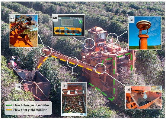
Figure 1.
Flow of coffee fruits in the harvester and details of the components of the yield monitor, temporary reservoir, and ultrasonic sensor (a); paddle conveyor (b); hydraulic motor (c); data logger (d); GNSS receiver (e); coffee wagon (f).
At the same time, an experiment was carried out to compare the data obtained with the yield monitor with the simultaneous weighing using a coffee wagon instrumented with load cells (Figure 2). The measurement of harvester yield data was carried out using a big-bag fixed to a metal structure supported on four load cells with individual reading capacity of up to 1000 kg and with an accuracy of 10 g, on a coffee wagon, similar to the work performed by [17]. The load cells were calibrated and connected to a data logger responsible for sending the data at a frequency of 5 Hz to a notebook that performed the integration with the positioning data obtained by a GNSS SMART6-L™ (NovAtel Inc., Calgary, AB, Canada) with TerraStar-C correction that results in an accuracy of ±0.09 m [25] (Figure 2e).
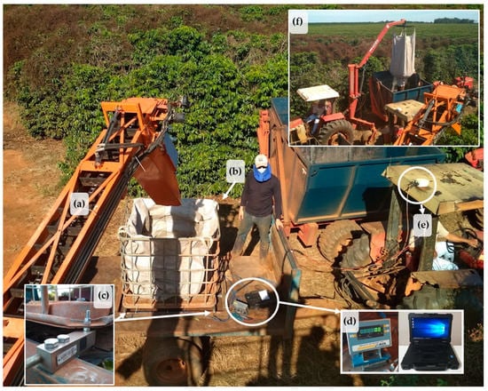
Figure 2.
Details of the coffee wagon instrumentation used to measure the harvester’s yield data, loading (a); big-bag (b); load cells (c); data logger (d); GNSS receiver (e); unloading (f).
The evaluation of the quality of the data generated by the monitor was carried out in two crop rows, one with low and the other with high yield of coffee fruits of the Catuaí 144 variety, with a spacing between lines of 4.0 m and 0.5 m between plants, with an approximate population of 5000 plants ha−1. In the low yield line, therefore, with low grain flow, data were collected in an extension of approximately 250 m and, in the high flow area, in an extension of approximately 87 m.
In order to compare the data obtained by the harvester and the load cells, it was necessary to standardize the frequency between the data obtained using the distance traveled as an adjustment factor. The data were analyzed with the addition of a standard offset according to the delay distance between the harvester and the instrumented wagon and the data without the offset. To compare the yield estimates performed by the yield monitor versus the load cells, a linear model was adjusted, and its coefficient of determination (R2) calculated.
To obtain the weight values of processed coffee (peeled and dried grains), it was necessary to obtain the CF. For this, 23, 44, and 31 samples were collected during the 2019, 2020, and 2021 harvests, respectively, at each coffee wagon, so random samples were collected throughout the area (Figure 3).

Figure 3.
Collection flow and processes for obtaining the CF.
Each sample consists of one liter of raw coffee that was weighed and sent to dry until it reached approximately 12% moisture and then peeled and weighed again to obtain the CF. The final weight of the processed coffee was determined using Equation (1):
where X is the yield of processed coffee (Mg ha−1); = volume accumulated over a time interval (L); is the distance traveled in the same time interval (m), W is the width of the coffee line (4 m), and CF is (kg L−1).
Yield data was filtered, eliminating headland maneuver data. Data close to roads that divide and cross the area and the discrepant data were filtered using the MapFilter 2.0 software using global filtering with a threshold of 100%, based on the methodology proposed by Maldaner and Molin [26].
Descriptive statistical and geostatistical analyses followed by visual assessment of yield maps were performed to identify patterns in spatial variability [27]. The variability expressed by the coefficient of variation (CV) was classified as low (CV < 12%), median (12% < CV < 62%), and high (CV > 62%), according to Warrick and Nielsen [28]. Spatial dependence index (SDI) was calculated from the semivariograms as C0/(C0 + C1), where C0 is the nugget variance (non-spatial variance), and C0 + C1 is the sill variance (spatially dependent variance). SDI was interpreted as strong (<0.25), moderate (between 0.25 and 0.75), or weak (>0.75), according to Cambardella et al. [29]. The model was determined based on the lowest root mean squared error (RMSE) value.
Yield data were interpolated using the software Vesper 1.6 [30] using the ordinary kriging method with a spatial resolution of 3.0 × 3.0 m. For the temporal analysis of the data, the interpolated maps were normalized with values 0 to 1 from Equation (2):
where xni is the normalized yield at point i of the grid, and xi is the yield at point i of the grid.
The identification of the temporal patterns of yield in the study area was first performed through the punctual correlation between the yield of the high-yield years. For this, the adjusted Pearson correlation coefficient was calculated for a linear model. At the same time, the normalized difference in yield between the years was calculated from Equation (3):
where is the normalized difference between the evaluated years, is the normalized yield at point i of the grid in year and is the normalized yield in grid point i in year .
To evaluate the temporal behavior and stability of yield between the years, the average temporal variance (Equation (4)) was calculated, following the methodology proposed by Blackmore et al. [31].
where: is the temporal variance at grid point i, t is the time in years between 2019 and 2021, Y is the yield in years t at point i, and is the mean of the yield for the whole field in years t.
3. Results and Discussion
3.1. Quality of Yield Data
In order to compare the data obtained by the yield monitor and the data obtained by the load cells, they were synchronized. This synchronization was necessary due to the path that the coffee fruits travel internally in the harvester. The harvest speed was approximately constant, and the displacement of the paddle conveyor was controlled by the ultrasound sensor, which depends on the amount of fruit being harvested. In this sense, it was necessary to adjust the distance between the beginning of the harvest and the beginning of the discharge to the coffee wagon.
The coffee wagon moved approximately 10 m until the first data was recorded by the harvester’s yield monitor. The behavior of the coffee fruit flow obtained in the high yield row (Figure 4a) shows that 519 L and 359 kg of coffee were harvested at a distance of approximately 87 m, representing a fruit flow of 5.96 L m−1 and 4.12 kg m−1, respectively. For the low-yield row (Figure 4b), the data indicated a harvest of 435 L and 331 kg of coffee in 219 m, corresponding to a flow of 1.98 L m−1 and 1.51 kg m−1, respectively, approximately three times lower than in the high-yield row. In addition, the distance lag between the beginning of the harvester’s data recording and the arrival of material on the instrumented wagon was approximately 36 m, a distance 3.6 times greater than in the high flow condition. In this case, higher variability in fruit flow was also observed. The first peak of variation was observed for both the load cells and by the yield monitor shortly after the arrival of the first fruits to the coffee wagon when the harvester was already in operation and the fruit flow suddenly increased.
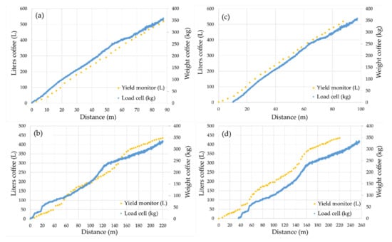
Figure 4.
Distribution of coffee fruit harvest data obtained by the yield monitor and by load cells in the (a) high- and (b) low-yield rows, and with the addition of offset in the distance to the load cells wagon in the (c) high- and (d) low-yield rows.
The high frequency of data collection obtained with the load cells on the wagon made it possible to clearly observe the variations in the flow of coffee fruits and, in some places, the offset between the data from the monitor and the load cells (Figure 4b). The fact that the measurement was made at different locations along with the coffee fruit flow most likely explains these differences. The ultrasonic sensor effectively controls the grain flow to ensure that the paddle conveyor compartments remain full until unloading. The load cells measure the mass flow being unloaded at the end of the paddle conveyor. The flicker effect is caused by the lack of harvested coffee fruit to fill the cells, causing the paddle conveyor to not move. Consequently, small variations in the comparison of signals are expected, as the systems are not measuring the flow of fruits harvested at the same location and with the mechanical interference of the flow by the yield monitor.
The results are also presented considering the addition of the offset in the distance between the harvester and instrumented wagon data. The offsets adopted were 10 m and 36 m for the high and low flow lines, respectively (Figure 4c,d). After correcting the load cells’ spatial offset, the data became more similar to those of the yield monitor, especially for the low flow line. Regardless, the yield monitor performed well in capturing the yield variability in the field.
The coffee fruit volume data obtained by the yield monitor and the fruit weight data obtained by the load cells on the wagon were initially correlated separately for each area without the addition of the offset. The fruit flow was regular for the high-yield row (Figure 5a), with no great variations in yield along the way, resulting in R2 of 0.995. In the low-yield row (Figure 5b), the R2 was 0.968. The joint analysis of the data referring to the two collections (Figure 5c) resulted in an R2 of 0.975, indicating a high correlation between the data obtained at high frequency by weighing and those on fruit volume obtained by the yield monitor at relatively low frequency.
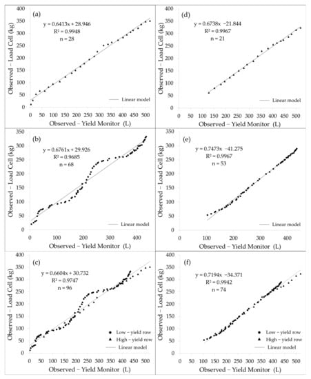
Figure 5.
Linear regression of coffee harvest data obtained by the yield monitor and by load cells for the (a,d) high-yield row, (b,e) low-yield row, (c,f) and all data together (a–c) before and (d–f) after correcting the offset.
As for the data considering the offset, the differences are small for the high-yield row (Figure 5d) when compared to those without the offset (R2 0.997), which can be explained by the constant and linear coffee fruit flow. For the low-yield row (Figure 5e), it is possible to notice a difference between the data that were not adjusted (Figure 5b). As the area presented greater variation in the fruit flow, the adjustment between the fruits leaving the harvester and the fruits entering the instrumented wagon proved to be efficient to perform the comparison, obtaining an R2 of 0.997. When the data from the two collections are grouped (Figure 5f), it is possible to observe a good fit, with R2 of 0.994.
The figures evidence the fact that the coffee mass data obtained from the load cells allowed greater detailing of the small flow changes during harvest. This behavior can be explained due to the low frequency in the collection of data from the yield monitor, as already observed by Maldaner et al. [32] when using an instrumented wagon to measure yield data in sugarcane harvesters.
3.2. Temporal and Spatial Yield Variability
The data referring to coffee fruit samples obtained in the field over the three harvests and the calculated CF are presented in Table 1. It was possible to observe that in the years 2019 and 2021, the area was harvested when more than 80% of the fruits were overripe or dry. On the other hand, the 2020 harvest happened when 49.1% and 22.2% of the coffee fruits were classified as ripe and unripe, respectively. Analyzing the results, the 1.0 L of coffee samples convert to a higher mass of dried and peeled grains when the harvest presented a higher percentage of overripe and dry coffee fruits, therefore, resulting in higher CF.

Table 1.
Coffee fruit weight, maturity stage, and CF from samples collected over three consecutive harvests (2019 to 2021).
As highlighted by Pezzopane et al. [33], as coffee fruits ripen, natural water loss is expected. Therefore, in the years 2019 and 2021, the amount of overripe coffee was greater and with the driest fruits. According to Silva et al. [34], unripe coffee has humidity between 60–70%, ripe coffee 45–55%, and overripe coffee 30–40%. In the harvest years of 2019 and 2021, the higher percentage of overripe fruits led to a coffee fruit density ranging between 470.0 and 492.5 g L−1. On the other hand, for the 2020 harvest, most of the fruits were in the ripe and unripe stages, resulting in an average coffee fruit density of 677.5 g L−1. This variation in the maturation stage also influences the size of the fruit. The overripe coffee fruits are usually smaller than the unripe and ripe coffee fruits, therefore, due to the smaller volume, more fruits are sampled per liter, resulting in higher CF values after drying and processing.
The need to obtain a CF from field samples to convert volume to yield data may be one of the factors limiting the adoption of yield monitors embedded in harvesters. As an alternative to this challenge, Bazame et al. [21] proposed the use of images associated with artificial intelligence to classify the grains and determine the stage of maturation in high spatial resolution.
During the 2019 harvest, data from some regions were not recorded by the yield monitor due to operational problems, resulting in a smaller amount of data when compared to the other years. However, even with this loss, the density of the filtered yield data ranged from 535 to 760 points ha−1. The density of data collection was still high when compared to scientific approaches that also aimed to identify spatial variability and map coffee yield. Ferraz et al. [14], Carvalho et al. [15], and Ferraz et al. [16] used manually collected point sampling techniques, and data collection ranged from 2.2 to 4.6 points ha−1.
Descriptive statistics of raw and filtered yield data are presented in Table 2. Data showed variations between years, with 2019 being the year with the lowest average yield (1.29 Mg ha−1). In the following year, the yield of processed coffee reached 2.03 Mg ha−1, and in 2021, it again decreased to 1.44 Mg ha−1. According to the classification of Warrick and Nielsen [28], the values of coefficient of variation (CV) ranging from 43.43% to 49.04% indicate that there is median variability in yield in the area. Carvalho et al. [15] highlighted that this may be a problem when only the average yield is considered for management decisions carried out for the entire area.

Table 2.
Descriptive statistics of yield data after filtering for the three evaluated crops.
Observing the average annual yield data, it is possible to identify the behavior of the crop, going from a year of low yield in 2019, to a year of high yield in 2020, and again showing low yield values in the following harvest (2021). In general, the coffee yield has a biennial behavior, with an alternation between a year of high yield, followed by a year of low yield. This variation is explained by the morphophysiological behavior of the coffee plant [35,36].
In addition to the biennial variability, the yield data for the three years also show a large yield spatial variability in the area (Figure 6). Several factors can influence this variability, including the biennial characteristic [4], the occurrence of diseases, pests and weeds [37,38,39], and soil fertility and foliar nutrition [40,41]. The biennial participation is expressive in the variation of the coffee yield. Due to the physiological characteristics of the plant, it must have high vegetative activity during one year, so that the following year it can produce well [5]. These high-density data (between 552.8 and 792.1 points ha−1) show this behavior of the crop with a high level of detail.
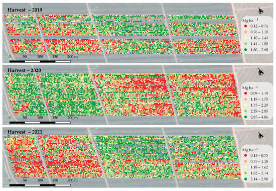
Figure 6.
Filtered processed coffee yield map data obtained by the yield monitor for the 2019 harvest; 2020 and 2021.
The semivariograms of yield data (Table 3) fitted exponential models with RSME of 0.022 Mg ha−1 for the 2019 harvest, with RSME of 0.011 Mg ha−1 for 2020 and 0.016 Mg ha−1 for 2021 using the Gaussian model. The spatial dependence index (SDI) was moderate, similar to the results found by Molin et al. [6], in which the authors used yield data obtained by a yield monitor and found a moderate SDI value fitted to the spherical model. In contrast, Carvalho et al. [15] collected point yield data samples, with a density of 4.5 points ha−1 at regular spacings and reported strong spatial dependence for yield in two seasons, with semivariograms fitted to a spherical model. Silva et al. [13], who sampled fruits of four plants around the crossing points of a sampling grid of 25 m (11 points ha−1) to calculate the average yield per plant, also found a strong spatial dependence for the yield of two coffee plantations by adjusting spherical models.

Table 3.
Semivariogram model and variables used to interpolate coffee yield data.
After adjusting the semivariograms, it was possible to estimate the yield in unsampled locations by interpolation and to standardize the size of each pixel of the maps for further spatial and temporal analysis.
The results of interpolation and normalization of yield data are shown in Figure 7. Regions with values close to 1 represent the maximum yield, while regions close to 0 represent the minimum yield for the year. A visual comparison shows some similarities between the years. The regions that had high yields in 2019 and 2021 were the same regions that had the lowest yields in 2020. Carvalho et al. [15] also observed similar results. The explanation for this alternation may be related to fruiting. Plants that produced a lot in 2019 (regions with green coloring in Figure 7) used their reserves for fruiting, negatively influencing the growth of branches and, consequently, reducing yield in 2020 (regions with red coloring in Figure 7). According to Matiello et al. [42], the coffee plant goes through a phase of low metabolism after high yields, and this behavior can cause this alternation of yield. It is important to point out that the biennial yield behavior is expressed inside and along the field, in addition to the spatial variability.
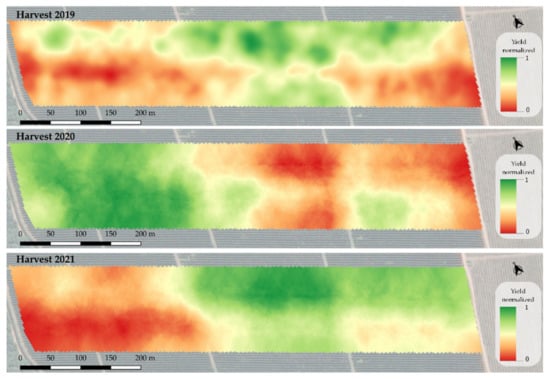
Figure 7.
Normalized yield map for the harvest in 2019, 2020, and 2021.
When the normalized yield data are individually compared among the years, it is possible to observe this yield alternation in the area. In consecutive years (Figure 8a,c) it is possible to notice the yield inversion pattern, presenting negative correlation values r of −0.53 when comparing between the harvests of 2019 and 2020, and r of −0.87 in the comparison between the harvests of 2020 and 2021. These results corroborate the results found by Carvalho et al. [15], which evaluated coffee yield over two years and also found a negative correlation between sequential years, with an r of −0.69. When the data from the odd years (2019 and 2021) are compared (Figure 8b), the behavior is opposite, with a positive correlation of r of 0.75. This indicates that there is an alternation of yield within the same area during the years and that the alternation regions are repeated.
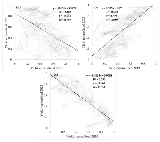
Figure 8.
Correlation of normalized yield data between crops of 2019 and 2020 (a), 2019 and 2021 (b), and 2020 and 2021 (c).
The maps of the normalized difference in yield are shown in Figure 9. Values close to 1 indicate that the region has a greater difference in yield between the years evaluated, whereas values close to 0 show a low difference in yield between the years. Likewise, in the correlation data, it was possible to notice the alternating behavior of yield between the sequential years 2019 and 2020 (Figure 9a) and 2020 and 2021 (Figure 9c). The map of the difference between the odd-numbered years (2019 and 2021) showed a result of low difference, indicating the similarity between the productive regions (Figure 9b). This yield difference between the years presents an additional degree of difficulty in managing the spatial variability of coffee plantations, since temporal variability influences and requires a longer sequence of data for a better understanding of the variability and for making decisions.
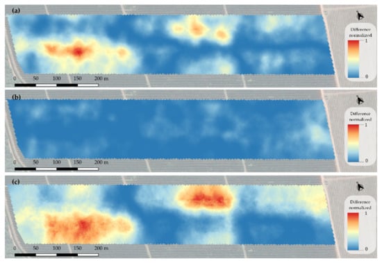
Figure 9.
Normalized difference map between yield data between crops 2019 and 2020 (a), 2019 and 2021 (b), and 2020 and 2021 (c).
Following the methodology proposed by [31], Figure 10 shows the map with the temporal variance yield for the three years evaluated. The regions that have the greatest variance in yield data are highlighted in the red areas, and the regions that have the most stability in yield data over the three years are highlighted in the blue areas. The regions with the highest variance were also the regions that showed the greatest differences between sequential years (Figure 9a,c). This result may indicate that, in addition to knowing the production variability, the variance information must also be considered in the strategies for site-specific management. The regions that presented high yield variance should possibly be conducted differently, receiving localized treatments alternated according to the productive year (high and low yield) and not only in consideration of their yield variability. As for the regions with low variance in the yield data, it is assumed that they present a more stable yield behavior over time, so they could be conducted taking into account only the yield variability.

Figure 10.
Yield map temporal variance along the three harvests.
4. Conclusions
The data obtained by the volumetric yield monitor embedded in a harvester showed a high correlation with those obtained with the load cells. This fact qualifies the yield data, allowing the identification of the fruit flow variation during harvest and the spatialization of these data to obtain reliable yield maps, with high data density.
It was possible to obtain yield data in a commercial area during three consecutive seasons, allowing the identification of its internal variability, as well as classifying regions that present alternating yields between the years evaluated. This result indicates that, in addition to knowing the spatial yield variability, the biennial variance information must also be considered in the strategies for site-specific management. Regions that presented high yield variance should be conducted differently, being alternated according to the productive year (high and low yield) and not only in consideration of their yield variability. This type of information helps in the search for possible causes of this variability so that the crop can be managed considering these spatial and temporal differences.
Future research to estimate coffee productivity using high-density data obtained by harvesters should consider faster and more assertive methods to identify the degree of fruit maturation, so, in addition to productivity, it would be possible to obtain a new layer regarding fruit quality, a subject that was not addressed in detail in this work and that is of great interest to coffee producers.
Author Contributions
Conceptualization, M.M. and J.P.M.; methodology, M.M., H.C.B. and J.P.M.; software, M.M. and H.C.B.; formal analysis, M.M. and H.C.B.; writing—original draft preparation, M.M., J.P.M. and H.C.B.; writing—review and editing, M.M., J.P.M. and H.C.B. All authors have read and agreed to the published version of the manuscript.
Funding
This research received no external funding.
Institutional Review Board Statement
Not applicable.
Informed Consent Statement
Not applicable.
Data Availability Statement
Not applicable.
Acknowledgments
To the Guima Café Group for allowing the use of their plantations as experimental areas and providing the people and machinery, Terrena Agronegócios for supporting the research, and the Coordination for the Improvement of Higher Education Personnel (in Portuguese: Coordenação de Aperfeiçoamento de Pessoal de Nível Superior—CAPES) for granting the scholarship of authors 1 and 3—Finance Code 001.
Conflicts of Interest
The authors declare no conflict of interest.
References
- Companhia Nacional de Abastecimento—(CONAB). Acompanhamento da Safra Brasileira: Café. 2021. Available online: https://www.conab.gov.br/component/k2/item/download/40314_5ca4f5eaec7d5fb8e90ec9645427e205 (accessed on 23 March 2022).
- Companhia Nacional de Abastecimento—(CONAB). Acompanhamento da Safra Brasileira: Café. 2022. Available online: https://www.conab.gov.br/component/k2/item/download/40911_0eac1d762da9a95acc3d8d4bd36d7359 (accessed on 23 March 2022).
- Santinato, F. Inovações Tecnológicas Para Cafeicultura de Precisão. Doctoral Thesis, Faculdade de Ciências Agrárias e Veterinárias—UNESP, Jaboticabal, São Paulo, Brazil, 2016; 125p. [Google Scholar]
- De Camargo, A.P.; de Camargo, M.B.P. Definition and outline for the phenological phases of arabic coffee under Brazilian tropical conditions. Bragantia 2001, 60, 65–68. [Google Scholar] [CrossRef]
- Rena, A.B.; Maestri, M. Fisiologia do cafeeiro. Inf. Agropecuário 1985, 11, 26–40. [Google Scholar]
- Molin, J.P.; Motomiya, A.V.D.A.; Frasson, F.R.; Faulin, G.D.C.; Tosta, W. Test procedure for variable rate fertilizer on coffee. Acta Scientiarum. Agronomy 2010, 32, 569–575. [Google Scholar] [CrossRef]
- Lowenberg-DeBoer, J.; Erickson, B. Setting the record straight on precision agriculture adoption. Agron. J. 2019, 111, 1552–1569. [Google Scholar] [CrossRef]
- Murugan, D.; Garg, A.; Singh, D. Development of an Adaptive Approach for Precision Agriculture Monitoring with Drone and Satellite Data. IEEE J. Sel. Top. Appl. Earth Obs. Remote Sens. 2017, 10, 5322–5328. [Google Scholar] [CrossRef]
- Molin, J.P.; Faulin, G.D.C. Spatial and temporal variability of soil electrical conductivity related to soil moisture. Sci. Agric. 2013, 70, 1–5. [Google Scholar] [CrossRef]
- Colaço, A.F.; Pagliuca, L.G.; Romanelli, T.L.; Molin, J.P. Economic viability, energy and nutrient balances of site-specific fertilization for citrus. Biosyst. Eng. 2020, 200, 138–156. [Google Scholar] [CrossRef]
- Molin, J.P.; do Amaral, L.R.; Colaço, A. Agricultura de Precisão, 1st ed.; Oficina de Textos: São Paulo, Brazil, 2015; p. 224. [Google Scholar]
- Rosa, V.G.C.; Moreira, M.A.; Rudorff, B.F.T.; Adami, M. Coffee crop yield estimate using an agrometeorological-spectral model. Pesqui. Agropecuária Bras. 2010, 45, 1478–1488. [Google Scholar] [CrossRef]
- Silva, F.M.; Souza, Z.M.; Figueiredo, C.A.P.; Vieira, L.H.S.; Oliveira, E. Spatial variability of chemical attributes and coffee productivity in two harvests. Ciência E Agrotecnologia 2008, 32, 231–241. [Google Scholar] [CrossRef]
- Ferraz, G.A.E.S.; da Silva, F.M.; Carvalho, L.C.C.; Alves, M.D.C.; Franco, B.C. Spatial and temporal variability of phosphorus, potassium and of the yield of a coffee field. Eng. Agric. 2012, 32, 140–150. [Google Scholar] [CrossRef]
- Carvalho, L.C.; Silva, F.M.; Ferraz, G.A.; Stracieri, J.; Ferraz, P.F.; Ambrosano, L. Geostatistical analysis of Arabic coffee yield in two crop seasons. Rev. Bras. Eng. Agrícola E Ambient. 2017, 21, 410–414. [Google Scholar] [CrossRef]
- Ferraz, G.A.E.S.; da Silva, F.M.; de Oliveira, M.S.; Custódio, A.A.P.; Ferraz, P. Spatial variability of plant attributes in a coffee plantation. Rev. Ciênc. Agron. 2017, 48, 81–91. [Google Scholar] [CrossRef]
- Balastreire, L.A.; Schueller, J.K.; Amaral, J.R.; Leal, J.C.G.; Baio, F.H.R. Coffee Yield Mapping. ASAE Annu. Meet. 2002. [Google Scholar] [CrossRef]
- Sartori, S.; Fava, J.F.M.; Domingues, E.L.; Ribeiro Filho, A.C.; Shiraisi, L.E. Mapping the spatial variability of coffee yield with mechanical harvester. In Proceedings of the World Congress on Computers in Agriculture and Natural Resources, Foz do Iguaçu, Paraná, Brazil, 13–15 March 2002; pp. 196–205. [Google Scholar] [CrossRef]
- Angnes, G.; Martello, M.; Faulin, G.D.C.; Molin, J.P.; Romanelli, T.L. Energy efficiency of variable rate fertilizer application in coffee production in Brazil. AgriEngineering 2021, 3, 815–826. [Google Scholar] [CrossRef]
- Faulin, G.C.; Molin, J.P.; Stanislavski, W.M. Sample density and method for obtaining of the correction factor used in the coffee (Coffea arabica L.) yield map. In Proceedings of the Congresso Brasileiro de Agricultura de Precisão—ConBAP, São Pedro, São Paulo, Brazil, 14–17 September 2014. [Google Scholar]
- Bazame, H.C.; Molin, J.P.; Althoff, D.; Martello, M. Detection, classification, and mapping of coffee fruits during harvest with computer vision. Comput. Electron. Agric. 2021, 183, 106066. [Google Scholar] [CrossRef]
- Santana, L.S.; Ferraz, G.A.e.S.; Teodoro, A.J.d.S.; Santana, M.S.; Rossi, G.; Palchetti, E. Advances in Precision Coffee Growing Research: A Bibliometric Review. Agronomy 2021, 11, 1557. [Google Scholar] [CrossRef]
- Alvares, A.C.; Stape, J.L.; Sentelhas, P.C.; Gonçalves, J.L.M.; Sparovek, G. Koppen’s climate classification map for Brazil. Meteorol. Z. 2013, 22, 711–728. [Google Scholar] [CrossRef]
- INMET. Brazil Climate Normals 1991–2020. 2022. Available online: https://portal.inmet.gov.br/normais (accessed on 30 April 2022).
- Maldaner, L.F.; Canata, T.F.; Dias, C.T.S.; Molin, J.P. A statistical approach to static and dynamic tests for Global Navigation Satellite Systems receivers used in agricultural operations. Sci. Agric. 2021, 78. [Google Scholar] [CrossRef]
- Maldaner, L.F.; Molin, J.P. Data processing within rows for sugarcane yield mapping. Sci. Agric. 2020, 77. [Google Scholar] [CrossRef]
- Colaço, A.F.; Molin, J.P.; Rosell-Polo, J.R.; Escolà, A. Spatial variability in commercial orange groves. Part 1: Canopy volume and height. Precis. Agric. 2019, 20, 788–804. [Google Scholar] [CrossRef]
- Warrick, A.W.; Nielsen, D.R. Spatial variability of soil physical properties in the field. In Applications of Soil Physics; Hillel, D., Ed.; Academic Press: New York, NY, USA, 1980; pp. 319–344. [Google Scholar]
- Cambardella, C.A.; Moorman, T.B.; Nowak, J.M.; Parkin, T.B.; Karlen, D.L.; Turco, R.F.; Konopka, A.E. Field-scale variability of soil properties in central Iowa soils. Soil Sci. Soc. Am. J. 1994, 58, 1501–1511. [Google Scholar] [CrossRef]
- Minasny, B.; Mcbratney, A.B.; Whelan, B.M. VESPER Version 1.62; Australian Centre for Precision Agriculture, McMillan Building A05; The University of Sydney: Sydney, Australia, 2005. [Google Scholar]
- Blackmore, S.; Godwin, R.J.; Fountas, S. The analysis of spatial and temporal trends in yield map data over six years. Biosyst. Eng. 2003, 84, 455–466. [Google Scholar] [CrossRef]
- Maldaner, L.F.; Canata, T.F.; Molin, J.P. An approach to sugarcane yield estimation using sensors in the harvester and zigbee technology. Sugar Tech 2021. [Google Scholar] [CrossRef]
- Gaspari-Pezzopane, C.D.; Medina Filho, H.P.; Bordignon, R.; Siqueira, W.J.; Ambrósio, L.A.; Mazzafera, P. Environmental influences on the intrinsic outturn of coffee. Bragantia 2005, 64, 39–50. [Google Scholar] [CrossRef]
- Silva, J.S.; Moreli, A.P.; Donzeles, S.M.L.; Soares, S.F.; Vitor, D.G. Harvesting, Drying and Storage of Coffee. In Food Engineering Series; Springer: Berlin/Heidelberg, Germany, 2021; pp. 1–64. [Google Scholar] [CrossRef]
- Pereira, S.O.; Bartholo, G.F.; Baliza, D.P.; Sogreira, F.M.; Guimarães, R.J. Growth, productivity and bienniality of coffee plants according to cultivation spacing. Pesqui. Agropecuária Bras. 2011, 46, 152–160. [Google Scholar] [CrossRef]
- Valadares, S.V.; Neves, J.C.L.; Rosa, G.N.G.P.; Martinez, H.E.P.; Venegas, V.H.A.; Lima, P.C. Productivity and biennial production of dense coffee plantations under diferente levels of N and K. Pesqui. Agropecuária Bras. 2013, 98, 296–303. [Google Scholar] [CrossRef]
- Fialho, C.M.T.; Silva, G.R.; Freitas, M.A.M.; França, A.C.; Mello, C.A.D.; Silva, A.A. Competition of weeds with coffee plants, in two times of infestation. Planta Daninha 2011, 28, 969–978. [Google Scholar] [CrossRef]
- Carvalho, A.M.; Mendes, A.N.; Botelho, C.E.; Oliveira, A.C.; Rezende, J.C.; Rezende, R.M. Agronomic performance of coffee cultivars resistant to coffee rust in Minas Gerais state, Brazil. Bragantia 2012, 71, 481–487. [Google Scholar] [CrossRef]
- Lopes, P.R.; Araújo, K.C.S.; Ferraz, J.M.G.; Lopes, I.M.; Fernandes, L.G. Producing agroecological coffee in Southern Minas Gerais: Alternative systems forintensive production of agrochemicals. Rev. Bras. Agroecol. 2012, 7, 25–38. [Google Scholar]
- Wadt, P.G.S.; Dias, J.R.M. Regional and inter-regional DRIS norms for nutritional evaluation of Conilon coffee. Pesqui. Agropecuária Bras. 2012, 47, 822–830. [Google Scholar] [CrossRef]
- Scalco, M.S.; Alvarenga, L.A.; Guimarães, R.J.; Dominghetti, A.W.; Colombo, A.; Assis, G.A.; Abreu, G.F. Leaf contents of phosphorus and zinc, productivity, and growth of irrigated coffee. Pesquisa Agropecuária Brasileira 2014, 49, 95–101. [Google Scholar] [CrossRef]
- Matiello, J.B.; Garcia, A.W.R.; Almeida, S.R. Adubação Racional na Lavoura Cafeeira, 1st ed.; Bom Pastor: Varginha, Brazil, 2008; p. 114. [Google Scholar]
Publisher’s Note: MDPI stays neutral with regard to jurisdictional claims in published maps and institutional affiliations. |
© 2022 by the authors. Licensee MDPI, Basel, Switzerland. This article is an open access article distributed under the terms and conditions of the Creative Commons Attribution (CC BY) license (https://creativecommons.org/licenses/by/4.0/).