Article

Spatial Variability of Production and Quality in Table Grapes ‘Flame Seedless’ Growing on a Flat Terrain and Slope Site

by
Nicolás Verdugo-Vásquez
1,
Emilio Villalobos-Soublett
1,
Gastón Gutiérrez-Gamboa
2,* and
Miguel Araya-Alman
3,*
1
Centro de Investigación Intihuasi, Instituto de Investigaciones Agropecuarias (INIA), Colina San Joaquín s/n, La Serena 1700000, Chile
2
Escuela de Agronomía, Facultad de Ciencias, Universidad Mayor, Huechuraba 8580000, Chile
3
Departamento de Ciencias Agrarias, Universidad Católica del Maule, km 6 Camino Los Niches, Curicó 3340000, Chile
*
Authors to whom correspondence should be addressed.
Horticulturae 2021, 7(8), 254; https://doi.org/10.3390/horticulturae7080254
Submission received: 31 July 2021 / Revised: 10 August 2021 / Accepted: 17 August 2021 / Published: 19 August 2021
(This article belongs to the Section Viticulture)

Abstract

:
(1) Background: Precision agriculture has been used mostly to study spatial variability in vineyards for winemaking. Nevertheless, there is little available information on the impacts of its use on table grape vineyards under different slope conditions. (2) Methods: The aim was to study the spatial variability of production and berry quality in ‘Flame Seedless’ vines established on a flat (3% slope) and sloping (23% slope) terrain in the Chilean hyper-arid northern region. (3) Results: The results showed that in both vineyards, the measured variables presented a high spatial variability according to their coefficient of variation, being higher in slope than in the flat vineyard. The geostatistical analysis showed that 82% of the measured variables presented a strong spatial dependence in the slope vineyard, whereas 45% and 55% of the variables measured in the flat vineyard presented strong and moderate spatial dependence, respectively. Elevation was related to berry quality parameters in both vineyards, while trunk vine circumference was related to berry quality for the slope vineyard and to yield for the flat vineyard. (4) Conclusions: There is an important spatial variability in table grape vineyards mostly those cultivated on slope sites. Therefore, precision agriculture tools can be useful for zoning table grape vineyards, and thus improving both economic returns of viticulturists and sustainability.

1. Introduction

Chile is the main table grape exporter in the world, with this crop accounting for a total of 53,523 ha of planted surface [1]. Table grapes are mostly cultivated in northern Chile under hyper-arid and semiarid conditions, where a severe reduction in irrigation water availability accompanied by temperature increases has been registered in the last decade [2]. Under these conditions, the main planted cultivar is ‘Flame Seedless’ [2,3]. Due to the geography of northern Chile, a significant portion of table grape production has been developed on sites that vary between 15 and 40% in slope, alongside flat vineyards (slope less than 5%).
During the last decade, several authors have postulated that in agriculture, and especially in viticulture, there is a high degree of spatial variability [4,5,6]. The use of precision agriculture tools in viticulture has made it possible to quantify the spatial variability of vineyards in several countries, including Chile [5,7,8], Uruguay [9], Australia [10], France [6], and Spain [11]. Some reports have revealed significant spatial variability in vineyards with respect to yield [12,13], bunch composition [14], vegetative growth [15], water status [7], and soil physicochemical characteristics [5]. However, these investigations were developed in vineyards planted for winemaking, and currently, there is scarce information available regarding spatial variability in vineyards for table grape production.
Some agronomical practices differ in vine management for table grape production compared to the practices employed in winemaking. Growth regulator applications and cluster thinning are essential practices that must be performed in order to obtain berries of a specific size and shape [16,17]. The production cycle of table grapes is shorter, since the harvesting of table grapes is usually performed when soluble solids reach between 15 and 17 ºBrix, while harvesting in winemaking usually takes place between 21 and 25 ºBrix [18,19]. These management differences could suggest that the variability of the yield components and berry quality parameters in a plot for table grape production could be less than those observed in a plot for vine cultivated for winemaking.
Despite the economic importance of table grape production in Chile and other producing countries, there are few available studies quantifying the spatial variability in table grape plots [20,21]. The quantification of spatial variability in table grape plots would make it possible to determine whether precision agriculture tools are useful and recommendable for use under this productive system. Therefore, the main goal of this study was to characterize the spatial variability of the production and berries quality of table grapes ‘Flame Seedless’ cultivated on flat and sloping terrain.

2. Materials and Methods

2.1. Experimental Site and Plant Material

Research was conducted in two commercial vineyards (Figure 1), belonging to the Agricultural Research Institute (INIA) planted with ‘Flame Seedless’ (Vitis vinifera L.) in the Vicuña Experimental Center, Elqui Valley, Coquimbo Region (30°02′ S, 70°41′ O, 630 m.a.s.l.) during the 2017–18 season.
Details about the characteristics of the vineyards with respect to total surface, rootstock selection, season of planting, and slope level, among others, are presented in Table 1. The vines were managed according to the conventional viticultural practices used in the Elqui Valley, in terms of leaf management, fertilization, growth regulator applications, irrigation, pruning and disease control.
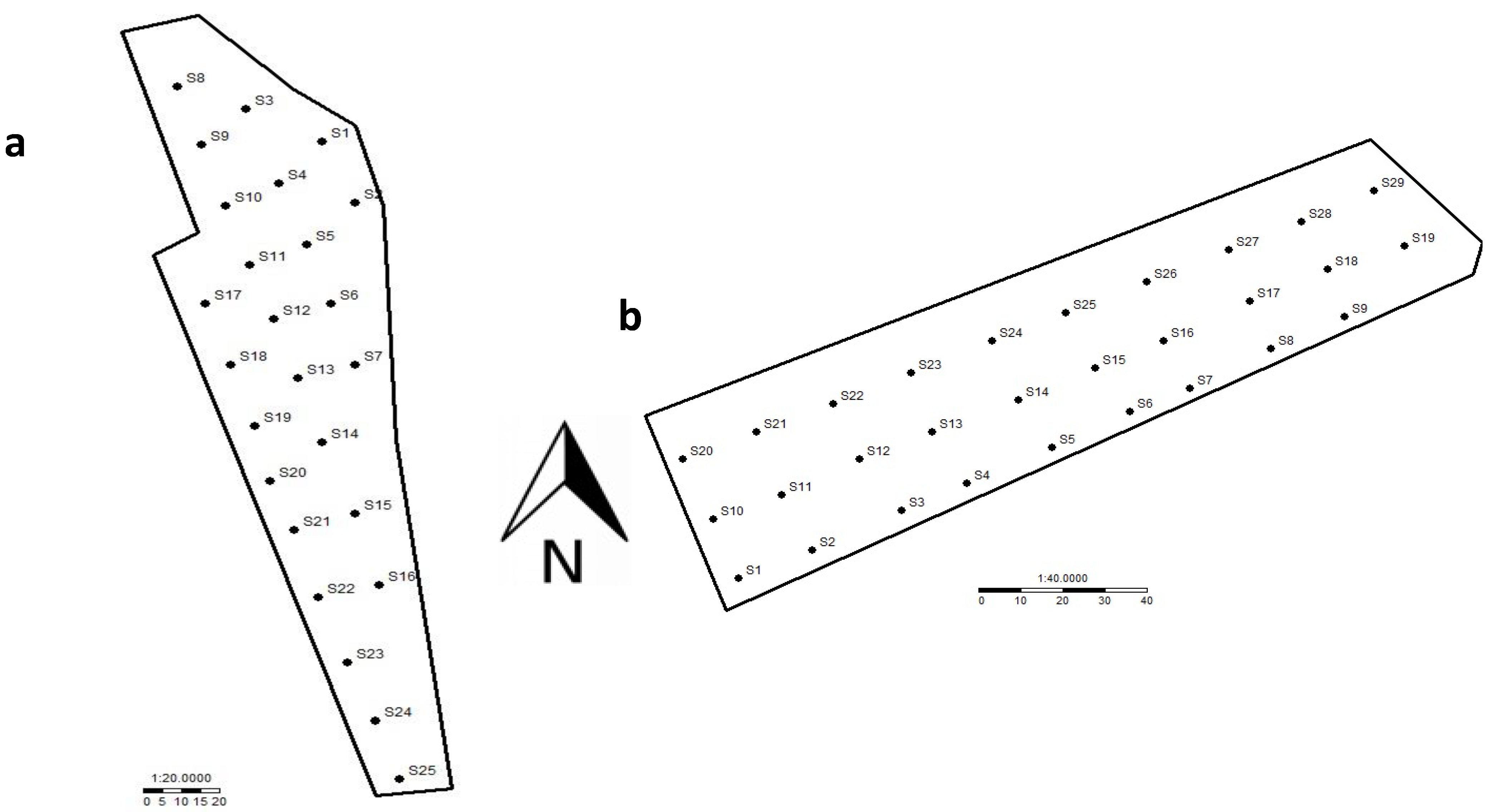
A regular sampling grid was designed within each plot (Figure 2) with 30 measurement sites per hectare (15 × 15 m). Based upon plot surface, the sampling grid considered 25 sites for the slope plot and 29 sites for the flat plot. Each site of the grid was represented by one plant. Sampling grid characteristics were conditioned by the operational restrictions related to the time required to perform the measurements in the vineyards. However, in the absence of other spatial information, given the average spatial variability of the yield in a wide number of vineyard plots [12], the sampling distance was enough to consider most of the of intra-plot variability. The borders of the fields and sampling sites within each field were geo-referenced with a differential global positioning system receiver (DGPS) (Trimble, Pathfinder ProXRS, Sunnyvale, CA, USA) and stored as Eastern and Northern coordinates (Datum WGS84, UTM projection, Zone 19S) to perform the mapping and spatial analysis. The elevation of each site was obtained from previous measurements (DGPS), and was expressed in meters above sea level.

2.2. Soil and Climate Conditions

Soil is classified as alluvial clay and belongs to the Entisol order [22]. The climatic characteristics of the study site were described in the reports published by Verdugo-Vásquez et al. [23,24]. Briefly, the zone under study is classified as hyper-arid (<100 mm annual rainfall average). Due to the low rainfall recorded during the season and the high vapor pressure deficit, it is necessary to apply water through irrigation.

2.3. Yield, Yield Components and Vine Vigor Parameters

The clusters of each sampling grid were manually harvested and weighed in a digital weight scale, recording yield per vine (kg vine−1) and the number of bunches per vine. The cluster weight (g) was obtained, dividing the yield per vine by the number of clusters per vine. In both plots, vines from the sampling grids were manually pruned in winter and the pruning weight (kg vine−1) was determined. Scion trunk circumference (cm) was measured at the end of each season (April) at 30 cm above the ground using a measuring tape.

2.4. Berry Quality Parameters

Measurements of total soluble solids (TSS) were performed weekly (from post-veraison) to define harvest in both plots. For each cluster, two berries were sampled at the top, the middle and the bottom of the cluster. The table grape harvest was determined when TSS reached close to 19 ºBrix in both plots. This last value corresponding to the optimal maturity at harvest to table grape producers in Elqui Valley. One sampling date for berry physicochemical parameters was considered, and it was performed at harvest by randomly selecting 100 berries from each site of the grid. TSS measurement was done using a thermo-compensating refractometer (BRIX30 model, Leica IFT 40, Fisher Scientific, Waltham, MA, USA), while pH and titratable acidity was determined using the OIV protocols [25]. Prior to the physicochemical measurements, the equatorial diameter (caliber, expressed in mm) of the 100 berries per site was determined, obtaining a value per site (average 100 berries). Maturity index was calculated as the relationship between TSS and titratable acidity [26].

2.5. Statistical Analysis

The analysis was performed according to the method described by Verdugo-Vásquez et al. [8]. Basic statistics such as standard deviation, and coefficient of variation (CV) were calculated. An analysis of variance (ANOVA) was carried out with the aim to find differences between the slope and flat plots for all the production and quality variables measured. Mean separation was performed by using Tukey test (p < 0.05) after verification of homogeneity of variance (Levene’s test). Yield, total soluble solids, berry weight and caliber data were subjected to a non-parametric test (Kruskal–Wallis test), since they did not comply with the assumption of homoscedasticity (Levene’s test). The analyzes were performed using the Xlstat Software version 2020.3.1 (Addinsoft SARL, Paris, France).
A semivariogram analysis was performed to study the spatial dependence of the measured variables in each plot. The computation of a semivariogram is usually not recommended with a low number of points (<100) [27]. However, for this experiment, the quality of data collected (manual measurements averaged over 100 berries) and the significant spatial organization of the fields allowed us to consider such analysis [8]. In these situations, the residual maximum likelihood (REML) variogram has been proposed because fewer data are required for the analysis [28]. The REML method is parametric and is considered reliable where there is trend in the data because it is based on generalized increments that filter trend out and only the covariance parameters are estimated [28]. Thus, omnidirectional semivariograms were calculated, and the three basic parameters of the semivariogram were obtained: nugget ( C 0 ), sill ( C 0 + C 1 ) and range (a), which define the degree and scale of spatial variation among the observations [8]. From semivariogram parameters the degree of spatial dependence also called the Cambardella index ( C I ), was derived by using the ratio between the nugget and the total semivariance of the semivariogram (sill), expressed as a percentage [29] as shown in Equation (1).
C I   ( % ) = [ C 0 C 0 + C 1 ] 100
The Cambardella index allowed us to compare the relative size of the nugget effect for each date of the experiment [29]. Thus, the values of C I < 25% indicate a strong spatial dependence; the values of C I 25% ≤ C I ≤ 75% indicate a moderate spatial dependence, and the values of C I > 75% correspond to a weak spatial dependence [30].
Mapping was performed according to the method described by Verdugo-Vásquez et al. [31]. Briefly, the interpolation method used in this study was based on a deterministic function (inverse distance weighting) with a power coefficient value (p = 0.5). Data mapping was performed with 3Dfield software (version 2.9.0.0., Copyright 1998–2007, Vladimir Galouchko, Moscow, Russia). Three classes were considered for each map: low (0 to 33% quantile), medium (34 to 67% quantile) and high (68 to 100% quantile).

2.6. Principal Component Analysis

A principal component analysis (PCA) was performed for the slope and flat plot, including all the measured variables in the sampling grids to define relationships between the plots and variables. The analyses were performed using the Xlstat Software version 2020.3.1 (Addinsoft SARL, Paris, France). In addition, maps of the first two factors of each PCA were also produced.

3. Results

3.1. Variability of Production and Quality of Table Grapes

Descriptive statistics for productive, berry physicochemical, and vine vigor parameters are presented in Table 2, Table 3 and Table 4. Regarding the yield and yield components (Table 2) both vineyards presented a high coefficient of variation, which was higher for the slope than the flat plot. Based on this, CV ranged from 8 to 34% in yield and yield components for the slope plot, whereas it varied from 4 to 16% in the flat plot (Table 2). Yield CV in the slope (34%) plot was more than the double than the flat (13%) plot. The analysis of variance showed significant statistical differences for the yield and yield components between both vineyards. Table grape cultivated in the flat plot presented higher yield, number of clusters, cluster weight and berry weight than the ones established in the slope plot (Table 2).
The descriptive statistics for the berry physicochemical parameters are presented in Table 3. There is a low CV for all the variables measured (Table 3), and in general, it was higher for the slope than the flat plot. Based on this, the CV ranged from 3 to 9% in berry physicochemical parameters for the slope plot, whereas it varied from 2 to 6% in the flat plot (Table 3). Total soluble solids (TSS) and caliber in table grapes from slope plot presented considerably higher CV (about double) than the ones collected from the flat plot. The analysis of variance showed significant statistical differences in most of the physicochemical parameters between both vineyards, except for total soluble solids (TSS). As expected, TSS did not show statistical differences between the plots. Titratable acidity and caliber were higher in the berries collected from the flat than from the slope vineyard (Table 3). pH and maturity index were higher in table grapes from the slope plot than in the ones from the flat plot (Table 3). In this way, significant statistical differences were found for the maturity index between the slope and the flat plots, which was probably associated with the differences in titratable acidity.
The descriptive statistics for the vine vigor parameters are presented in Table 4. There are small differences on CV for each of the measured variables. Trunk circumference did not show statistical differences between the vines cultivated in the slope and flat plots. Pruning weight was higher in the vines growing in the slope plot than in the ones established in the flat plot.

3.2. Spatial Dependence Characterization of Production and Quality of Table Grapes

Geostatistical analysis is presented in Table 5. Most of the measured variables presented moderate and strong spatial dependence, according to Cambardella Index. In this way, 82% of the variables showed a strong spatial dependence in the slope vineyard, whereas 45 and 55% of the measured variables presented a strong and moderate spatial dependence in the flat vineyard, respectively. The number of clusters and pH were the variables that presented a weak spatial dependence in the slope plot, while the rest of the parameters presented a strong spatial dependence. The yield, total soluble solids, pH, maturity index, and vigor parameters presented a moderate spatial dependence in the flat plot, whereas the rest of the parameters presented a strong spatial dependence.
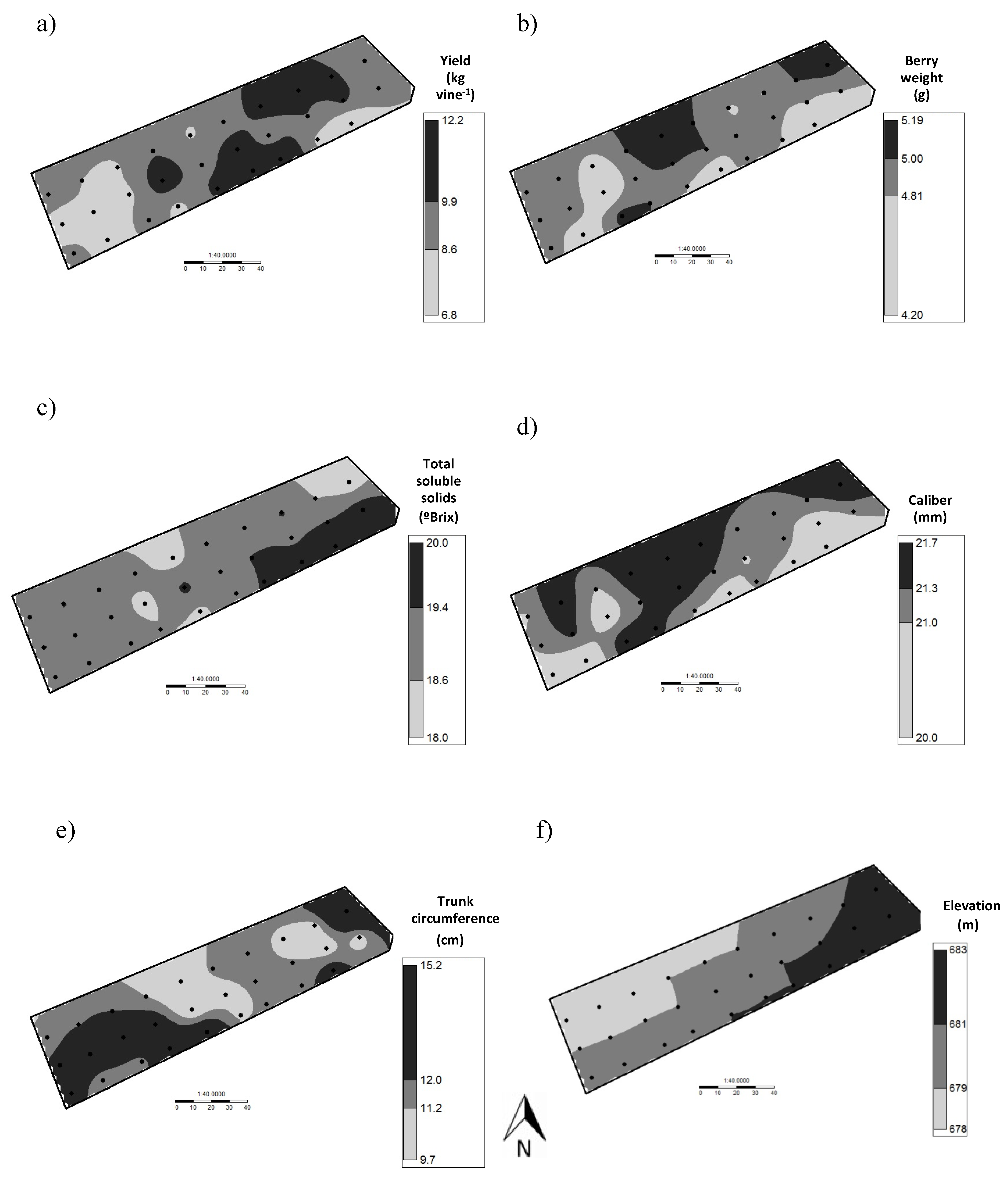
Figure 3 and Figure 4 show maps of yield, berry weight, total soluble solids, caliber, trunk circumference and elevation measured in the slope and flat vineyards, respectively. Based on the results presented in Figure 3, the slope vineyard presented a variability with a high spatial structure, confirming the results of the geostatistical analysis (Table 5). In general, the low quartile (0 to 33% quartile presented in light gray color) was the one that presented the highest spatial structure. Total soluble solids (Figure 3c) and elevation (Figure 3f) were the variables that presented the highest spatial structure, where each class is represented by a specific area within the vineyard.
Based on the results presented in Figure 4, the variability of the flat vineyard had a consistent spatial structure. In general, the classes are represented by more than one zone within the plot (Figure 4). In this way, total soluble solids (Figure 4c) and elevation (Figure 4f) were the variables that presented the highest spatial structure, a result also observed for the slope vineyard. On the other hand, similarities between the maps of the slope and flat vineyards were observed (Figure 3 and Figure 4). Both vineyards presented similar spatial patterns of elevation alike to those observed for total soluble solids.

3.3. Multivariate Analysis of the Measured Variables by Plot

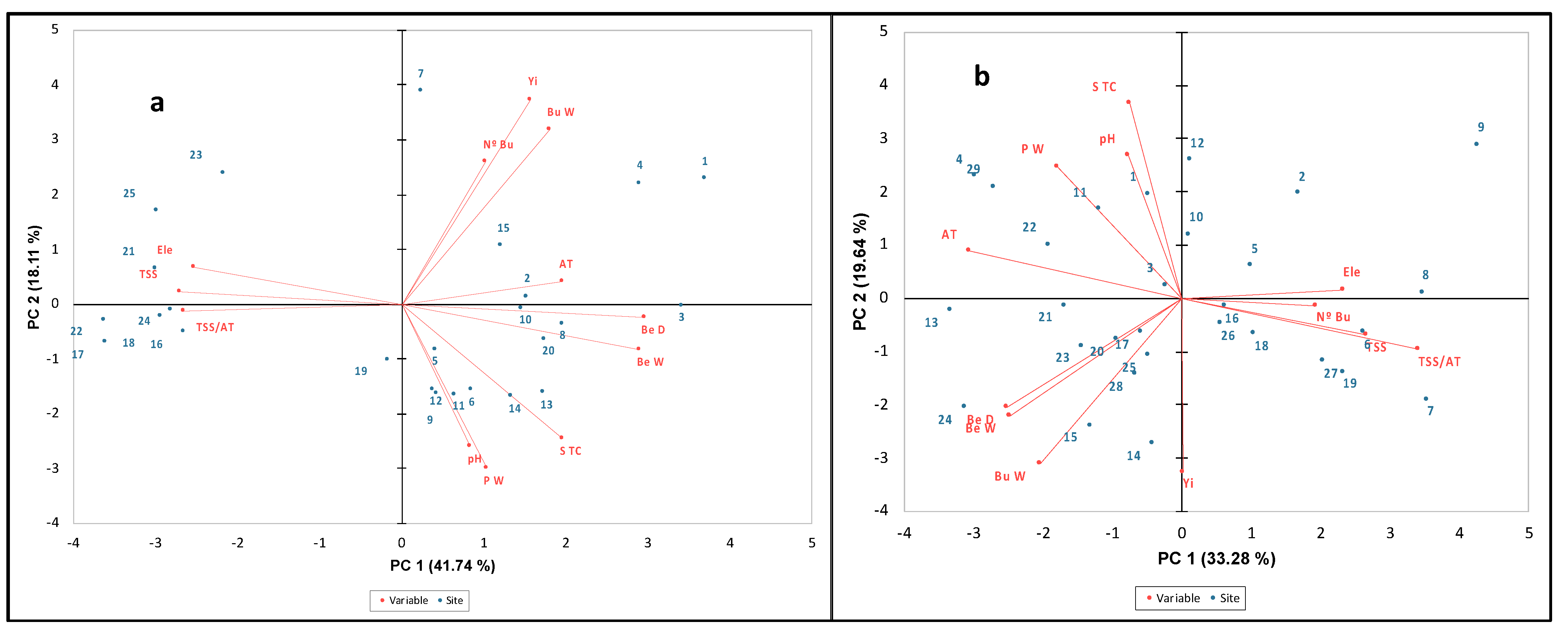
Two principal component analyses (PCA) were performed, including all available data for the slope (Figure 5a) and flat (Figure 5b) vineyards. As for the slope vineyard, principal component 1 (PC 1) explained 41.7% of the variance, and principal component 2 (PC 2) explained 18.1%, representing a 59.8% of all the variance. PC 1 was most correlated with fruit physicochemical parameters, elevation, and trunk circumference, while PC 2 was correlated with productive parameters (yield and bunch weight). Trunk circumference was positively correlated with caliber, berry weight, and pruning weight, while it was negatively correlated with plot elevation.
Concerning the flat vineyard, PC 1 explained 33.3% of the variance, and PC 2 explained 19.6%, representing a 52.9% of all the variance. PC 1 was most correlated with caliber, total soluble solids (TSS), maturity index, titratable acidity, and elevation, while PC 2 was correlated with yield and vigor parameters. Trunk circumference was positively correlated with pruning weight, and negatively related to bunch weight.
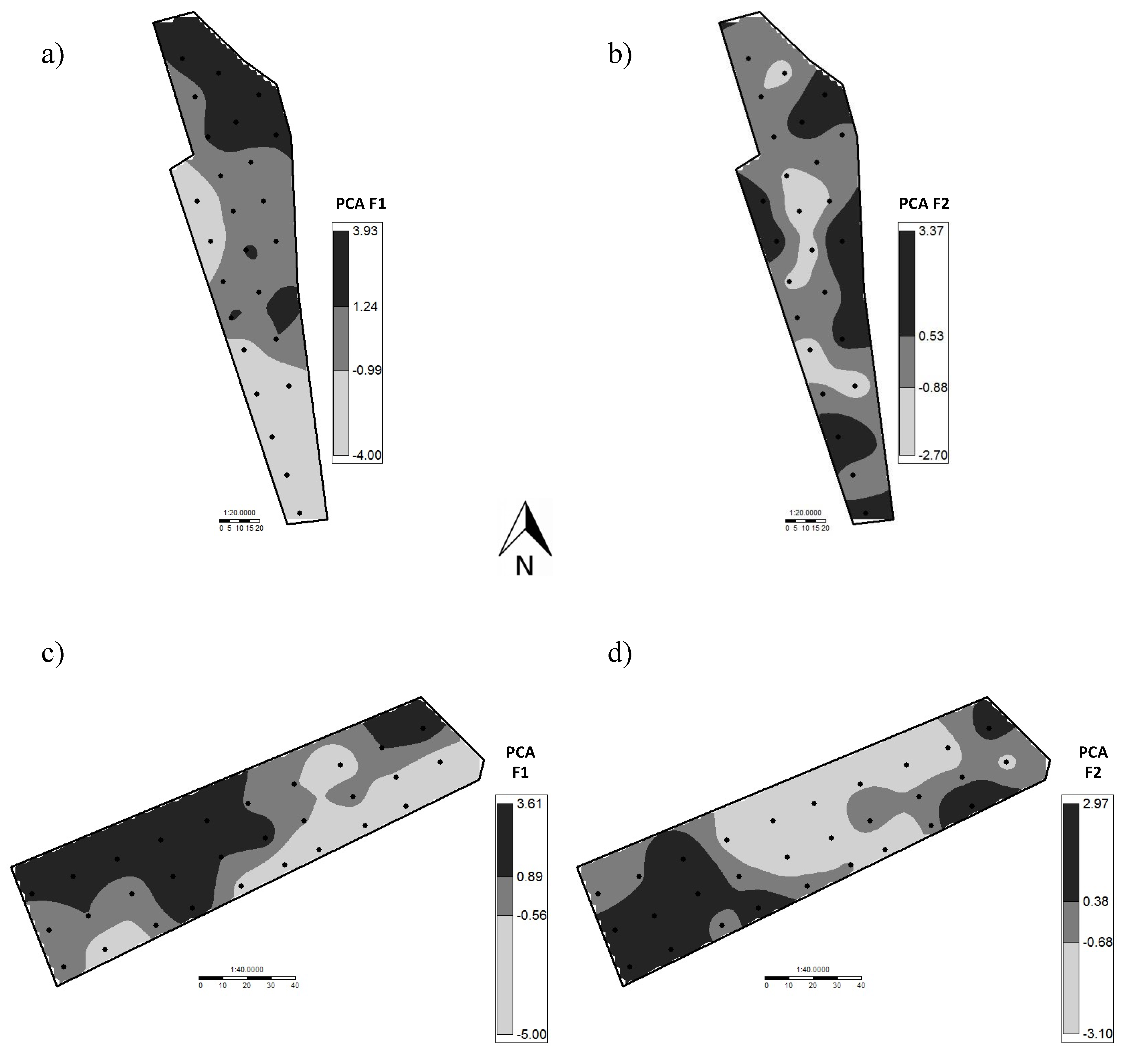
To determine if the distribution of the sampling sites along the components of each PCA has a spatial structure, the information of both components was mapped for the slope and the flat vineyards under study (Figure 6). Based on these results, mapping of component 1 (Figure 6a,c) presents a higher spatial structure than the component 2 (Figure 6b,d). Concerning the slope vineyard (Figure 6a), the southern zone (low quartile represented by light gray color) was characterized by being the upper zone of the plot (high elevation) and is marked by having a high accumulation of total soluble solids, but low weight and caliber. Contrary to this, the south-west zone (low quartile represented by light gray color) of flat plot (Figure 6c) was characterized by a slightly higher elevation, which was associated with berries with high values of total soluble solids and low values of acidity.

4. Discussion

Based on the results described, most of the measured variables, and the productive parameters most of all, presented a higher degree of variability (as coefficient of variation) in the slope than in the flat vineyard (Table 2, Table 3 and Table 4). A similar percentage of variability was reported by Anastasiou et al. [21] on yield components in table grapes ‘Thompson Seedless’ cultivated in southern Greece. However, several reports have pointed out that the percentage of variability in the parameters measured in grapevines cultivated for winemaking is higher than that observed in this study for table grapes [5,12,13,31]. These differences may be associated with the cultural practices that must be performed in each productive system, i.e., table or wine grapes. Some practices such as crop thinning and application of growth regulators must be mandatorily performed in table grape production, which may reduce yield variability. With respect to berry physicochemical parameters, similar values of percentage of variability have been reported in table grape [21] and in wine grape production [11,31]. With respect to vine vigor parameters, trunk circumference did not show significant differences between the two plots (Table 4). Based upon the results, there is an important variability in table grape production under the conditions of northern Chile, mostly in vineyards established on slope terrains. Moreover, there were significant differences in several of the measured variables, where the flat vineyard presented the best commercial results in terms of yield and berry caliber. Based on multivariate analysis, the elevation was correlated with berry quality variables in the slope and the flat vineyards. Moreover, trunk circumference was correlated with berry quality variables in the slope plot and with yield in the flat vineyard. The elevation corresponds to a permanent and stable variable of the plots, and it could be used to perform differential management zones, if the spatial patterns observed for the quality variables are stable among seasons.
These preliminary results made it possible to characterize the spatial variability of table grape established in vineyards with different slope degree under the hyper-arid conditions of the Elqui Valley. In this first study, the spatial variability of parameters measured directly in the plants was considered. However, to complement the description of the spatial variability of table grape production systems, soil measurements (texture, depth, organic matter, among others) and other factors such as the orientation of the vineyard, size of the fields, type of pruning, among others, should be considered.
This information can be useful as the basis for the development of future research: (i) To use auxiliary information measured at high spatial resolution for zoning the vine plots. Similar studies examining this information have been developed in Chile [5] and in France [32] in vineyards for wine production. (ii) To characterize the microclimate of the plants. In this sense, the results of this study can bring us practical information for determining the location at which the temperature and humidity sensors should be positioned. This information could help to explain the seasonal differences in yield, yield components and berry physicochemical parameters observed within each vineyard. Dahal et al. [20] mentioned that inconsistent yield between seasons for table grape cultivars presents a challenge to the industry in terms of marketing and economic sustainability. These authors suggested that seasonal yield variation in some varieties could be associated with the effect of high temperature during inflorescence initiation and early development which occurs in the studied location. Verdugo-Vásquez et al. [8] showed that the microclimatic information measured in the plants made it possible to explain the differences in phenology and accumulation of total soluble solids observed at the intra-plot scale in grapevine varieties cultivated in the Maule Valley. Currently, there are low-cost alternatives for monitoring the temperature at the plant level; information that can be used to model phenological states of the vines [33]. (iii) To define sampling strategies. The results obtained in the Figure 5 and Figure 6 can be used to define the best sampling sites for the key variables or the ones that accounts a strong degree of spatial dependence in table grape management, such as productive parameters and some berry physicochemical parameters. (iv) To determine the stability of the studied zones in the following seasons. The measurements of the variables should be performed during at least three future seasons, which would make it possible to determine if the zones defined in Figure 3 and Figure 4 are stable over time, as has been reported for the accumulation of soluble solids in grapes from vineyards cultivated in the Maule Valley [31]. This information could be used to propose spatial models, which allow simplifying the spatial representation of a certain variable, using as little information as possible. In this fashion, spatial models have been proposed for the vine water status [7], the accumulation of soluble solids in grape berries [31] and vine phenological stages [34]. This knowledge will make it possible to improve the sustainability of table grape production, by being able to perform site-specific management in the production systems.

5. Conclusions

To our knowledge, this is the first study highlighting the spatial variability of the yield and quality table grapes, growing under the hyper-arid conditions of northern Chile. Based on the results, there was high spatial variability in the slope and flat plots, which was structured in both situations. The geostatistical analysis revealed that most of the measured variables presented a strong spatial dependence in the slope vineyard, whereas some of the variables measured in the flat vineyard presented a strong and moderate spatial dependence. Thus, correlations found between the variables allowed to zone the plots. The above information can be used to propose new studies or to establish sampling strategies that consider spatial variability, mostly in the table grapes cultivated in slope plots to contribute to the sustainability and the saving of the table grape industry. At last, we think that it is of great importance to perform investigations over more seasons and under different edaphoclimatic conditions to establish better conclusions regarding the spatial variability of table grapes.

Author Contributions

Conceptualization, N.V.-V.; methodology, N.V.-V. and M.A.-A.; software, N.V.-V. and M.A.-A.; validation, N.V.-V. and M.A.-A.; formal analysis, E.V.-S., G.G.-G., N.V.-V. and M.A.-A.; investigation, N.V.-V. and M.A.-A.; data curation, E.V.-S., G.G.-G. and N.V.-V.; writing—original draft preparation, N.V.-V., G.G.-G. and M.A.-A.; writing—review and editing, N.V.-V., G.G.-G., E.V.-S. and M.A.-A.; visualization, N.V.-V. and G.G.-G.; supervision, N.V.-V. project administration, N.V.-V. All authors have read and agreed to the published version of the manuscript.

Funding

This research received external funding from VRIP-UCM.

Acknowledgments

The authors are also grateful to Antonio Ibacache, Elizabeth Pastén, Carmen Jopia and Nelson Rojas for their valuable technical support.

Conflicts of Interest

The authors declare no conflict of interest.

References

  1. SAG Catastro Vitícola Nacional. Available online: http://www.sag.cl/ambitos-de-accion/catastro-viticola-nacional/1490/publicaciones (accessed on 30 November 2020).
  2. Ibacache, A.; Albornoz, F.; Zurita-Silva, A. Yield responses in Flame seedless, Thompson seedless and Red Globe table grape cultivars are differentially modified by rootstocks under semi arid conditions. Sci. Hortic. 2016, 204, 25–32. [Google Scholar] [CrossRef]
  3. Ibacache, A.; Sierra, C. Influence of rootstocks on nitrogen, phosphorus and potassium content in petioles of four table grape varieties. Chil. J. Agric. Res. 2009, 69, 503–508. [Google Scholar] [CrossRef] [Green Version]
  4. Trought, M.C.T.; Bramley, R.G.V. Vineyard variability in Marlborough, New Zealand: Characterising spatial and temporal changes in fruit composition and juice quality in the vineyard. Aust. J. Grape Wine Res. 2011, 17, 79–89. [Google Scholar] [CrossRef]
  5. Ortega-Blu, R.; Molina-Roco, M. Evaluation of vegetation indices and apparent soil electrical conductivity for site-specific vineyard management in Chile. Precis. Agric. 2016, 17, 434–450. [Google Scholar] [CrossRef]
  6. Tisseyre, B.; Mazzoni, C.; Fonta, H. Whithin-field temporal stability of some parameters in viticulture: Potential Toward a Site Specific Management. OENO One 2008, 42, 27–39. [Google Scholar] [CrossRef]
  7. Acevedo-Opazo, C.; Valdés-Gómez, H.; Taylor, J.A.; Avalo, A.; Verdugo-Vásquez, N.; Araya, M.; Jara-Rojas, F.; Tisseyre, B. Assessment of an empirical spatial prediction model of vine water status for irrigation management in a grapevine field. Agric. Water Manag. 2013, 124, 58–68. [Google Scholar] [CrossRef]
  8. Verdugo-Vásquez, N.; Acevedo-Opazo, C.; Valdés-Gómez, H.; Araya-Alman, M.; Ingram, B.; García de Cortázar-Atauri, I.; Tisseyre, B. Spatial variability of phenology in two irrigated grapevine cultivar growing under semi-arid conditions. Precis. Agric. 2016, 17, 218–245. [Google Scholar] [CrossRef]
  9. Fourment, M.; Ferrer, M.; González-Neves, G.; Barbeau, G.; Bonnardot, V.; Quénol, H. Tannat grape composition responses to spatial variability of temperature in an Uruguay’s coastal wine region. Int. J. Biometeorol. 2017, 61, 1617–1628. [Google Scholar] [CrossRef] [PubMed]
  10. Bramley, R.G.V. Understanding variability in winegrape production systems 2. Within vineyard variation in quality over several vintages. Aust. J. Grape Wine Res. 2005, 11, 33–42. [Google Scholar] [CrossRef]
  11. Baluja, J.; Tardaguila, J.; Ayestaran, B.; Diago, M.P. Spatial variability of grape composition in a Tempranillo (Vitis vinifera L.) vineyard over a 3-year survey. Precis. Agric. 2013, 14, 40–58. [Google Scholar] [CrossRef] [Green Version]
  12. Taylor, J.A.; Tisseyre, B.; Bramley, R.G.V.; Reid, A. A comparison of the spatial variability of vineyard yield in European and Australian production systems. In Proceedings of the 5th European Conference on Precision Agriculture, Uppsala, Sweden, 9–12 June 2005; pp. 907–915. [Google Scholar]
  13. Araya-Alman, M.; Leroux, C.; Acevedo-Opazo, C.; Guillaume, S.; Valdés-Gómez, H.; Verdugo-Vásquez, N.; Pañitrur-De la Fuente, C.; Tisseyre, B. A new localized sampling method to improve grape yield estimation of the current season using yield historical data. Precis. Agric. 2019, 20, 445–459. [Google Scholar] [CrossRef]
  14. Bramley, R.G.V.; Siebert, T.E.; Herderich, M.J.; Krstic, M.P. Patterns of within-vineyard spatial variation in the ‘pepper’ compound rotundone are temporally stable from year to year. Aust. J. Grape Wine Res. 2017, 23, 42–47. [Google Scholar] [CrossRef]
  15. King, P.D.; Smart, R.E.; McClellan, D.J. Within-vineyard variability in vine vegetative growth, yield, and fruit and wine composition of Cabernet Sauvignon in Hawke’ s Bay, New Zealand. Aust. J. Grape Wine Res. 2014, 20, 234–246. [Google Scholar] [CrossRef]
  16. Dokoozlian, N.K.; Hirschfelt, D.J. The influence of cluster thinning at various stages of fruit development on Flame Seedless table grapes. Am. J. Enol. Vitic. 1995, 46, 429–436. [Google Scholar]
  17. Lynn, C.D.; Jensen, F.L. Thinning effects of bloomtime gibberellin sprays on Thompson Seedless table grapes. Am. J. Enol. Vitic. 1966, 17, 283–289. [Google Scholar]
  18. Jayasena, V.; Cameron, I. °Brix/acid ratio as a predictor of consumer acceptability of Crimson Seedless table grapes. J. Food Qual. 2008, 31, 736–750. [Google Scholar] [CrossRef]
  19. Gutiérrez-Gamboa, G.; Zheng, W.; Martínez de Toda, F. Strategies in vineyard establishment to face global warming in viticulture: A mini review. J. Sci. Food Agric. 2020, 101, 1261–1269. [Google Scholar] [CrossRef]
  20. Dahal, K.C.; Bhattarai, S.P.; Midmore, D.J.; Oag, D.R.; Walsh, K.B. Temporal yield variability in subtropical table grape production. Sci. Hortic. 2019, 246, 951–956. [Google Scholar] [CrossRef]
  21. Anastasiou, E.; Tsiropoulos, Z.; Balafoutis, T.; Fountas, S.; Templalexis, C.; Lentzou, D.; Xanthopoulos, G. Spatiotemporal stability of management zones in a table grapes vineyard in Greece. Adv. Anim. Biosci. 2017, 8, 510–514. [Google Scholar] [CrossRef]
  22. Balbontín, C.; Campos, I.; Odi-Lara, M.; Ibacache, A.; Calera, A. Irrigation performance assessment in table grape using the reflectance-based crop coefficient. Remote Sens. 2017, 9, 1276. [Google Scholar] [CrossRef] [Green Version]
  23. Verdugo-Vásquez, N.; Gutiérrez-Gamboa, G.; Villalobos-Soublett, E.; Zurita-Silva, A. Effects of rootstocks on blade nutritional content of two minority grapevine varieties cultivated under hyper-arid conditions in Northern Chile. Agronomy 2021, 11, 327. [Google Scholar] [CrossRef]
  24. Verdugo-Vásquez, N.; Gutiérrez-Gamboa, G.; Díaz-Gálvez, I.; Ibacache, A.; Zurita-Silva, A. Modifications induced by rootstocks on yield, vigor and nutritional status on Vitis vinifera Cv Syrah under hyper-arid conditions in northern Chile. Agronomy 2021, 11, 979. [Google Scholar] [CrossRef]
  25. OIV. International Code of Oenological Practices; International Organization of Vine and Wine: France, Paris, 2020. [Google Scholar]
  26. Muñoz-Robredo, P.; Robledo, P.; Manríquez, D.; Molina, R.; Defilippi, B.G. Characterization of sugars and organic acids in comermercial varieties of table grape. Chil. J. Agric. Res. 2011, 71, 452–458. [Google Scholar] [CrossRef] [Green Version]
  27. Oliver, M.A. Geostatistical Applications for Precision Agriculture; Springer: Dordrecht, The Netherlands, 2010; ISBN 9789048191321. [Google Scholar]
  28. Kerry, R.; Oliver, M.A. Comparing sampling needs for variograms of soil properties computed by the method of moments and residual maximum likelihood. Geoderma 2007, 140, 383–396. [Google Scholar] [CrossRef]
  29. Cambardella, C.A.; Moorman, T.B.; Parkin, T.B.; Karlen, D.L.; Novak, J.M.; Turco, R.F.; Konopka, A.E. Field-scale variability of soil properties in central iowa soils. Soil Sci. Soc. Am. J. 1994, 58, 1501–1511. [Google Scholar] [CrossRef]
  30. Wu, C.; Wu, J.; Luo, Y.; Zhang, L.; DeGloria, S.D. Spatial prediction of soil organic matter content using cokriging with remotely sensed data. Soil Sci. Soc. Am. J. 2009, 73, 1202–1208. [Google Scholar] [CrossRef]
  31. Verdugo-Vásquez, N.; Acevedo-Opazo, C.; Valdés-Gómez, H.; Ingram, B.; De Cortázar-Atauri, I.G.; Tisseyre, B. Temporal stability of within-field variability of total soluble solids of grapevine under semi-arid conditions: A first step towards a spatial model. OENO One 2018, 52, 15–30. [Google Scholar] [CrossRef] [Green Version]
  32. Acevedo-Opazo, C.; Tisseyre, B.; Guillaume, S.; Ojeda, H. The potential of high spatial resolution information to define within-vineyard zones related to vine water status. Precis. Agric. 2008, 9, 285–302. [Google Scholar] [CrossRef] [Green Version]
  33. Fuentes-Peñailillo, F.; Acevedo-Opazo, C.; Ortega-Farías, S.; Rivera, M.; Verdugo-Vásquez, N. Spatialized system to monitor vine flowering: Towards a methodology based on a low-cost wireless sensor network. Comput. Electron. Agric. 2021, 187, 106233. [Google Scholar] [CrossRef]
  34. Verdugo-Vásquez, N.; Acevedo-Opazo, C.; Valdés-Gómez, H.; Ingram, B.; Garcia de Cortázar-Atauri, I.; Tisseyre, B. Towards an empirical model to estimate the spatial variability of grapevine phenology at the within field scale. Precis. Agric. 2019, 21, 107–130. [Google Scholar] [CrossRef]
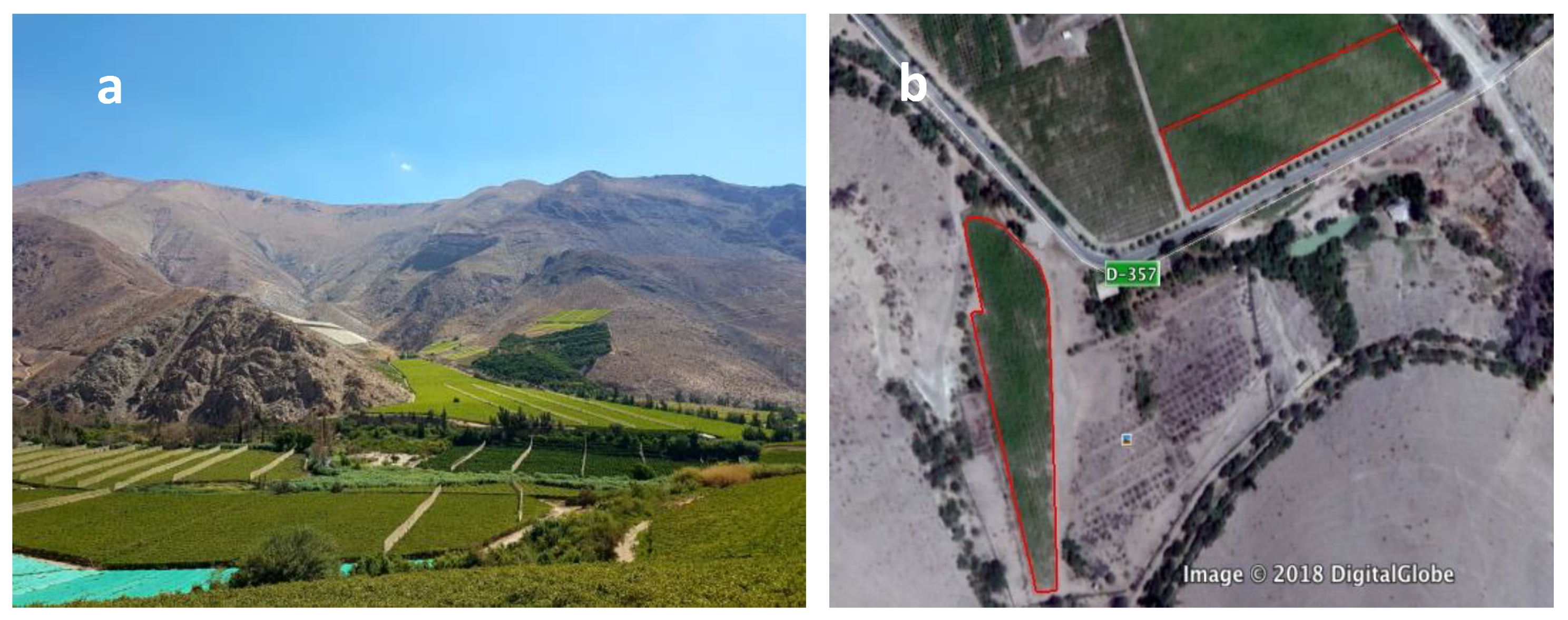
Figure 1. Production of table grapes on slopes and flat areas typical of northern Chile (a). The slope (lower left) and flat (top right) vineyards under study (b).
Horticulturae 07 00254 g001
Figure 2. Measurement grids used in the experiment. The 25 grid sites for the slope plot (a) and 29 grid sites for flat plot (b). Si represents the sampling site number i.
Horticulturae 07 00254 g002
Figure 3. Maps of the main variables determined in table grapes cultivated in the slope plot. (a) Yield, (b), berry weight, (c) total soluble solids, (d) caliber, (e) trunk circumference, (f) elevation.
Horticulturae 07 00254 g003
Figure 4. Maps of the main variables determined in table grapes cultivated in the flat plot. (a) Yield, (b), berry weight, (c) total soluble solids, (d) caliber, (e) trunk circumference, (f) elevation.
Horticulturae 07 00254 g004
Figure 5. Principal component analysis for slope (a) and flat (b) vineyards, including all the measured variables. Nomenclature: Ele: Elevation. TSS: Total soluble solids. TSS/AT: Maturity index. N° Bu: Number of clusters. Yi: Yield Bu W: Cluster weight. AT: Titratable acidity. STC: Trunk circumference. PW: Pruning weight. Be D: Caliber. Be W: Berry weight.
Horticulturae 07 00254 g005
Figure 6. Map of the two first components of each principal component analysis (PCA) for slope (a,b), and for flat (c,d) plot. (a,c) Component 1; (b,d) component 2. Each class (grayscale) corresponds to 33% of the data. F1 = PC 1 and F2 = PC 2.
Horticulturae 07 00254 g006
Table 1. Main characteristics of the table grapes under study.
PlotSlope (%)Surface
(ha)
RootstockYear of PlantingTrellis SystemPlanting Distance (m)
Slope230.95Harmony2015Overhead3 × 2
Flat30.98
Table 2. Descriptive statistics and analysis of variance (ANOVA) for the yield and yield components of the slope and flat plots under study.
PlotStatisticNumber of ClustersYield
(kg vine−1)
Cluster Weight (kg)Berry Weight (g)
SlopeMean15.0 a6.0 a0.40 a4.65 a
Standard deviation3.42.00.070.38
CV (%)22.933.616.958.11
FlatMean17.1 b9.3 b0.55 b4.88 b
Standard deviation2.71.20.080.21
CV (%)15.812.814.34.27
Significance******
CV: Coefficient of variation. For a given factor and significance p < 0.05, different letters within a column represent significant differences (Tukey’s test, p < 0.05). Yield and berry weight data were subjected to a non-parametric test (Kruskal–Wallis test). ns: No significant, *: Significant (p < 0.05), **: highly significant (p < 0.01).
Table 3. Descriptive statistics and analysis of variance (ANOVA) for the berry physicochemical parameters of the slope and flat plots under study.
PlotStatisticTSS (°Brix)Titratable Acidity (%)pHMaturity IndexCaliber (mm)
SlopeMean19.230.63 a3.67 b30.65 b20.5 a
Standard deviation0.970.030.102.760.61
CV (%)5.05.042.699.012.96
FlatMean19.020.72 b3.49 a26.57 a21.2 b
Standard deviation0.510.030.101.720.38
CV (%)2.664.853.006.471.79
Significancens********
CV: Coefficient of variation. ns: not significant. TSS: Total soluble solids. For a given factor and significance p < 0.05, different letters within a column represent significant differences (Tukey’s test, p < 0.05). TSS and caliber data were subjected to a non-parametric test (Kruskal–Wallis test). ns: No significant, **: highly significant (p < 0.01).
Table 4. Descriptive statistics and analysis of variance (ANOVA) for the vine vigor parameters of the slope and flat plots under study.
PlotStatisticTrunk Circumference (cm)Pruning Weight (kg vine−1)
SlopeMean12.255.74 b
Standard deviation1.311.70
CV (%)10.7229.46
FlatMean11.794.22 a
Standard deviation1.191.24
CV (%)10.1029.66
Significancens**
CV: Coefficient of variation. ns: not significant. For a given factor and significance p < 0.05, different letters within a column represent significant differences (Tukey’s test, p < 0.05). ns: No significant, **: highly significant (p < 0.01).
Table 5. Spatial dependence (Cambardella index) of the measured variables in the plots under study.
Cambardella Index
SlopeFlat
Measured VariableValue (%)Spatial DependenceValue (%)Spatial Dependence
Number of clusters100Weak20.5Strong
Yield1.7Strong49.9Moderate
Cluster weight0.2Strong17.1Strong
Total soluble solids0.1Strong27.7Moderate
Titratable acidity7.4Strong19.6Strong
pH100Weak33.2Moderate
Berry weight10.4Strong0.24Strong
Caliber0.26Strong10.9Strong
Maturity index0.11Strong50Moderate
Trunk circumference23.1Strong35.5Moderate
Pruning weight19.8Strong40.1Moderate
Publisher’s Note: MDPI stays neutral with regard to jurisdictional claims in published maps and institutional affiliations.