A Machine Learning Model for Photorespiration Response to Multi-Factors

Abstract

Photorespiration results in a large amount of leaf photosynthesis consumption. However, there are few studies on the response of photorespiration to multi-factors. In this study, a machine learning model for the photorespiration rate of cucumber leaves’ response to multi-factors was established. It provides a theoretical basis for studies related to photorespiration. Machine learning models of different methods were designed and compared. The photorespiration rate was expressed as the difference between the photosynthetic rate at 2% O₂ and 21% O₂ concentrations. The results show that the XGBoost models had the best fit performance with an explained variance score of 0.970 for both photosynthetic rate datasets measured using air and 2% O₂, with mean absolute errors of 0.327 and 0.181, root mean square errors of 1.607 and 1.469, respectively, and coefficients of determination of 0.970 for both. In addition, this study indicates the importance of the features of temperature, humidity and the physiological status of the leaves for predicted results of photorespiration. The model established in this study performed well, with high accuracy and generalization ability. As a preferable exploration of the research on photorespiration rate simulation, it has theoretical significance and application prospects.

1. Introduction

Photosynthesis is a crucial factor in crop yield formation. Besides the extrinsic factors such as microclimate around the crop, including light intensity [1,2], CO₂ concentration [3], temperature [4], and humidity [5], there are many intrinsic factors affecting the rate of photosynthesis, such as photorespiration, leaf age, chlorophyll content, and genes. In particular, photorespiration is a process closely related to photosynthesis, which physiologically reduces the efficiency of photosynthesis. The enzyme ribulose-1,5-bisphosphate carboxylase/oxygenase (RuBisCO) catalyzes the addition of CO₂ to ribulose-1,5-bisphosphate (RuBP), forming two 3-phosphoglycerate (3-PGA), which is called the carboxylation reaction. However, in C3 plants, a part of the enzyme RuBisCO oxidizes RuBP to 2-phosphoglycolate (2-PG) that is harmful to the plant and needs to be metabolized, thus causing waste and reducing the efficiency of photosynthesis [6]. In recent decades, many researchers have suggested the possibility of manipulating photorespiration in terms of modern biotechnology [7,8,9,10,11], while it remains a major challenge in applying biotechnological approaches in crop production. Instead of genetic editing and breeding, physical methods to reduce photorespiration can produce results instantly, and only require an understanding of how it changes with the environment.

Photorespiration is influenced by the surrounding environment, similar to photosynthesis. Most obviously, the ambient CO₂ concentration is closely related to the rate of photorespiration because O₂ acts as a competitive inhibitor for RuBisCO, i.e., the higher the ambient CO₂ concentration, the less photosynthesis efficiency reduced by photorespiration. Like most other enzymes, the kinetic properties of Rubisco highly depend on temperature, and the correlation varies among different plants [12,13]. This results in generally higher rates of oxygenation and higher losses of carbon from photorespiration at higher leaf temperatures [14]. Studies have shown that the rate of photorespiration is increased with high light intensities [15,16,17]. In addition, humidity also influences the rate of photorespiration. Then, it becomes possible to control the environment to reduce the consumption of photosynthesis by photorespiration. For example, in greenhouse production or a closed system, slow release of dry ice can be applied to increase the concentration of CO₂ in the air.

Photosynthesis models were greatly interesting to many researchers over a period of decades, since most of the dry matter of fruits originates from carbohydrate molecules produced by photosynthesis. In contrast, photorespiration models have received little attention from researchers. It has been extensively discussed in literatures that the response of photosynthesis to a specific environmental factor varies with plant species. For photosynthesis–irradiance curves, non-rectangular hyperbolic or rectangular hyperbolic models have been commonly used. Ye [18] and Ye et al. [19] developed an alternative model with additional restriction terms to improve the fit. Lanoue et al. [20] studied the translocation of Solanum lycopersicum cv. assimilates with differing spectral quality. The Farquhar–von Caemmerer–Berry (FvCB) model has been proposed for over 40 years [21], and the worldwide studies and improvements on the model had made significant progress [22,23,24]. Considerable results were accumulated using the model for fitting net assimilation rate–intercellular space CO₂ concentration (A–Ci) curve and the estimation of photosynthetic biochemical parameters [25,26,27,28]. In field, irradiance changes all the time, which makes the static assimilation model no longer accurate, and the dynamic model developed to solve the problem [29,30]. For photosynthetic response models with multiple environmental factors, summarizing mechanistic models is more difficult when the dimensionality of the dependent variable is higher, whereas empirical models are easier to implement and have been widely studied. Li et al. [31] described the daily variation of photosynthesis with temperature and photosynthetically active radiation (PAR) in greenhouse cucumber. Peri et al. [32] studied the photosynthetic response of Berberidaceae to light intensity, water status, and leaf age. Zhang and Wang [33] simulated a model of canopy photosynthesis in greenhouse tomato based on simple leaf photosynthesis. While empirical models are mostly built with the help of traditional statistical methods, a new type of approach, designed to make the most accurate predictions possible—machine learning—is gradually gaining attention. Goltsev et al. [34] developed a neural network (NN) model to show the relationship between chlorophyll fluorescence and the effect of water stress on leaf photosynthetic processes. Heckmann et al. [35] evaluated the potential of leaf reflectance spectroscopy to predict parameters of photosynthetic capacity in Brassica oleracea and Zea mays using a two-layer NN. Jian et al. [36] established tomato population photosynthetic rate prediction models based on support vector regression (SVR), and the correlation coefficient reached a maximum of 0.9883. Zhang et al. [37] compared the effectiveness of several machine learning approaches in predicting photosynthetic rates from leaf phenotypes, with the extreme gradient boosting (XGBoost) performing the best. Although these studies have contributed to the application of machine learning models of photosynthesis, barely anyone has studied models of the effects of photorespiration on photosynthesis.

Photorespiration is so important, but it is often ignored and undiscussed by those who study photosynthesis models. Although the response of photorespiration to a single environmental factor has been studied in depth [38,39,40,41], its response to multiple environmental factors has been little studied. Currently, there is no effective and convenient method and evaluation index to assess the negative effects of photorespiration. Additionally, the determination of the photorespiration rate is mostly based on complex physiological experiments [42], which require a lot of time and resources and cannot be used quickly and directly in production practice. Consequently, there is an urgent need for available methods to rapidly assess the amount of photorespiration and its effect on photosynthesis rates.

Therefore, taking greenhouse cucumbers (Cucumis sativus L.) as an example and based on the previous machine learning model of photosynthesis, this study focused on photorespiration, and established a model of the response of photorespiration to multiple environmental factors, thus achieving an accurate estimation of the negative effects of photorespiration. In the meantime, the effects of environmental factors on photorespiration were analyzed, hence the impact factors that need particular attention were found. Machine learning methods such as polynomial regression, k-nearest neighbors (KNN), Gaussian process (GP), SVR, adaptive boosting (Adaboost), gradient boosting decision tree (GBDT), XGBoost, and NN were used to fit the relationship between environmental factors and photorespiration. The modeling effects of different approaches are compared. This study investigated using machine learning methods with different environmental conditions to predict photorespiration rate at different leaf positions in two growth stages (seedling and flowering-fruit stages) of cucumber. It will provide a theoretical basis for studies related to photorespiration.

2. Materials and Methods

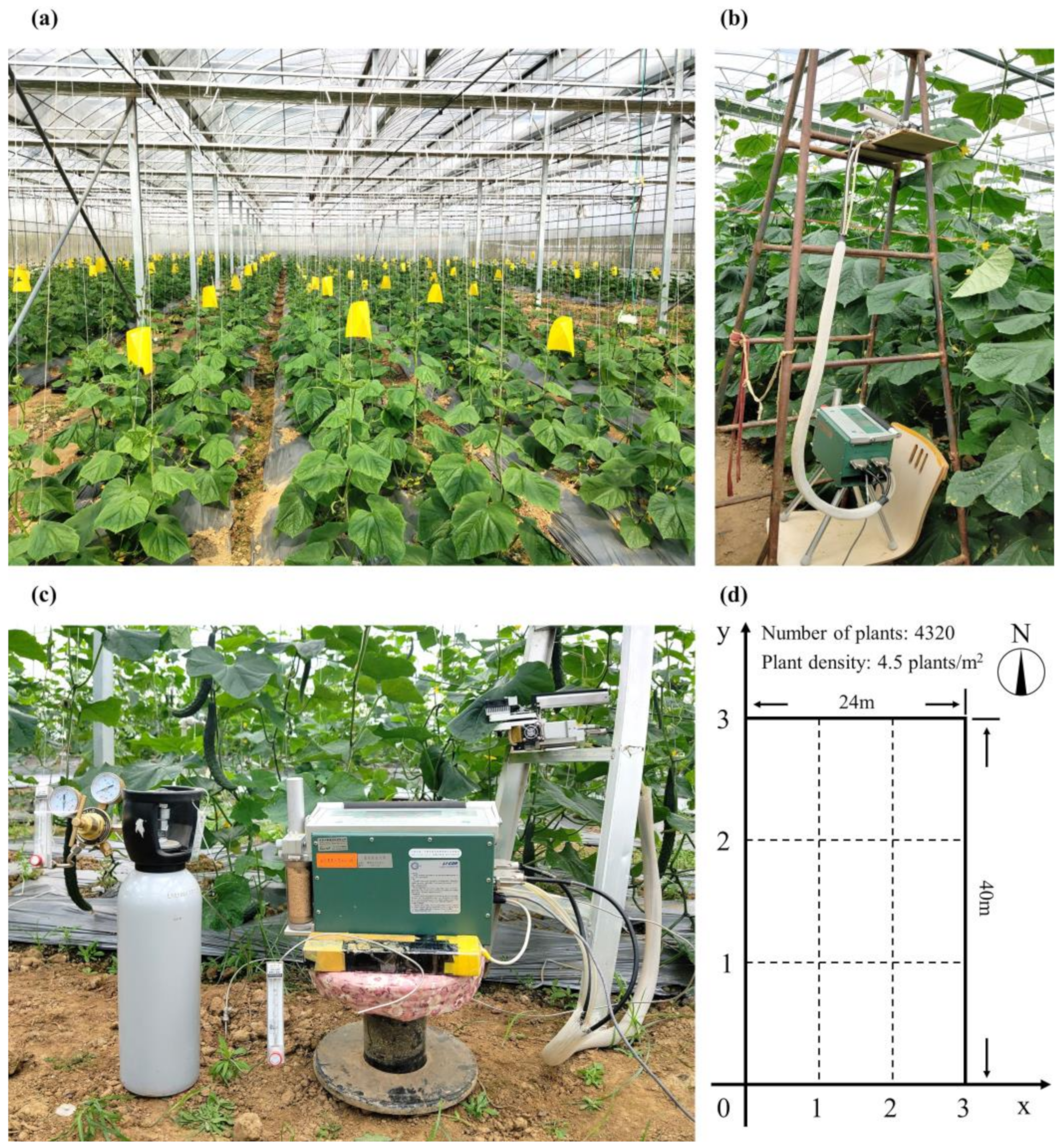
2.1. Data Access

Cucumber, an annual creeping vine plant in the Cucurbitaceae gourd family, is an important cash crop widely cultivated in temperate and tropical regions around the world [43]. In this study, cucumber was used as the subject of the photorespiration model. The cultivar of cucumber for experiment was ‘Jingyou 409’, a northern Chinese variety. The experiment was conducted in a plastic greenhouse of Baima Teaching and Research Base, Nanjing Agricultural University, Nanjing, China (31°36′ N, 119°10′ E). The mono-cropping system of cucumber was cropped twice in spring (April to July) and fall (September to November) of the year 2020, with a density of 4.5 plants/m² (Figure 1a). During the experimental period, fertigation, pest control and environmental control measures are taken according to cucumber production routines. Plants of much the same progress and conditions were selected for measurement by simple random sampling at seedling stages and the flowering-fruit stage.

Photosynthetic parameters in cucumber leaves were measured using LI-6400XT Portable Photosynthesis System, manufactured by LI-COR, USA (Figure 1b). To avoid the influence of midday depression on data collection, the experiment was conducted from 8:00–11:00 and 14:00–17:00 daily. The CO₂ injector and LED leaf chamber modules of LI-6400XT created the CO₂ concentration and photosynthetically active radiation (PAR, substituted by photosynthetic photon flux density, PPFD) in the microclimate, respectively. CO₂ concentration gradients of 200–800 ppm and PAR gradients of 0–2000 μmolm⁻²s⁻¹ are set using the AutoPrograms. Then, humidity and temperature were measured by the greenhouse environmental parameters at the same time. To reduce measurement error, the leaves of three adjacent cucumber plants were randomly selected for measurement in each group of environmental conditions. Leaf positions 1, 3, 5, 7 and 9 of each cucumber plant were selected (counting from the first fully expanded individual leaf from growing point) for measurement. The location of each tested plant in the greenhouse was also recorded.

One realizable approach to quantifying photorespiration in field is to suppress it by supplying the leaf with only 2% O₂ (instead of the normal 21% O₂) and measure the increased rates of photosynthesis [42]. An air tank with only 2% O₂ was connected to the air inlet of the LI-6400XT, where it was vented to the atmosphere through a T-fitting on the pipe, to prevent the internal pump from fighting against the external tank pressure (Figure 1c).

A total of 4550 sets of data were obtained from these measurements, which were used to form the initial dataset. A total of seven independent variables, features (PAR, CO₂ concentration, temperature, humidity, growth stage, leaf position, plant location), and one dependent variable, label (photosynthetic rate with the effect of photorespiration and photosynthetic rate without the effect of photorespiration), were included.

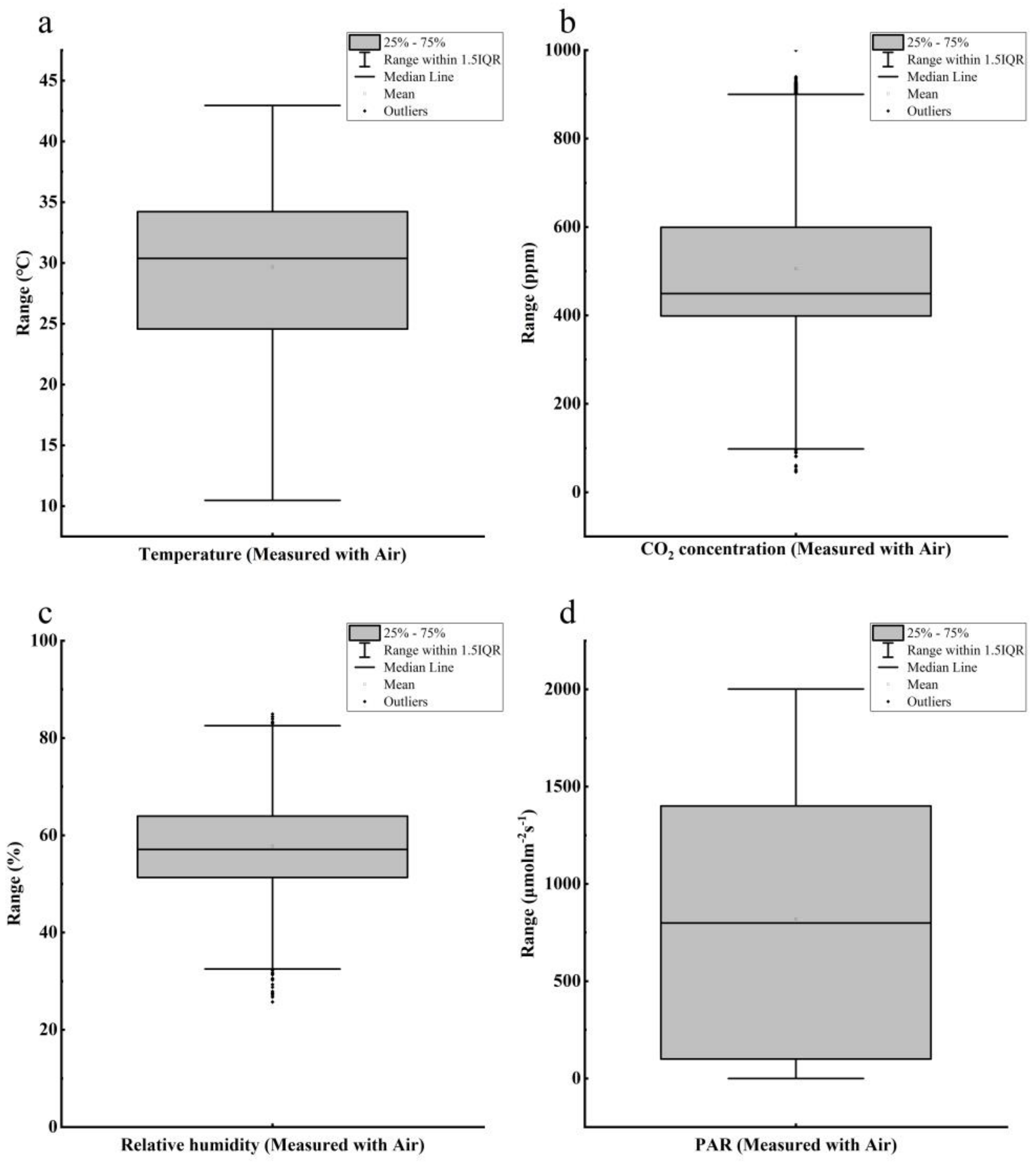
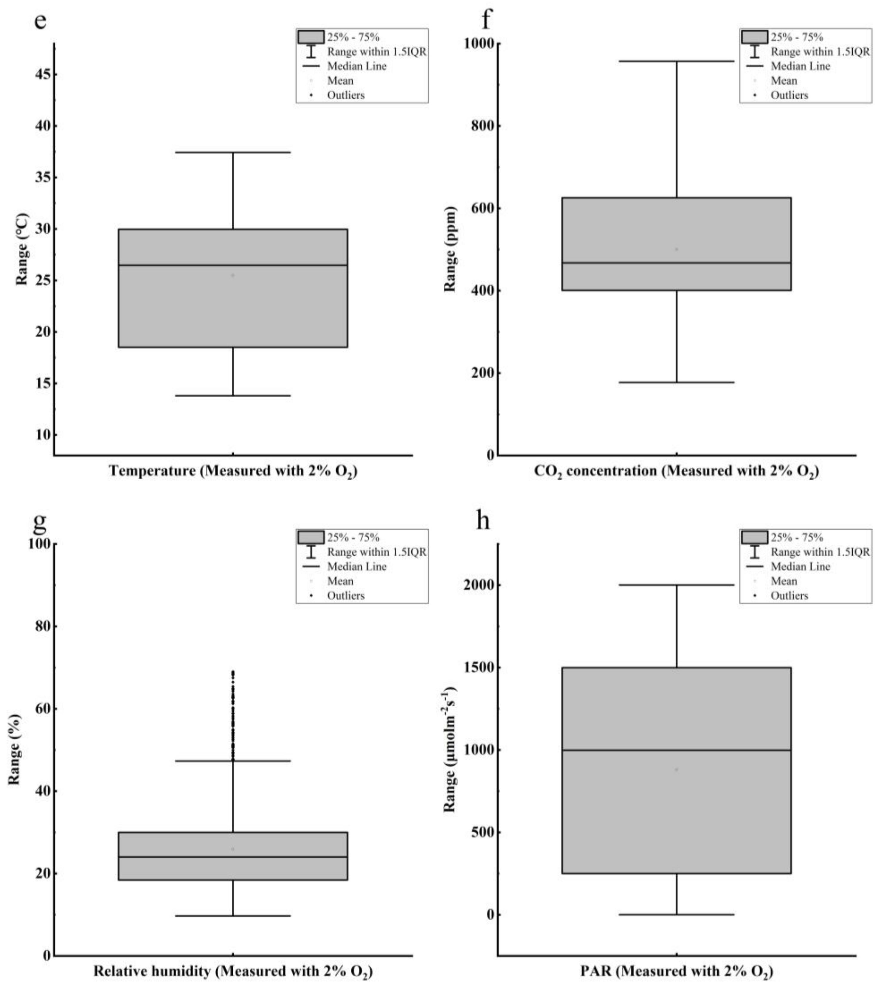
2.2. Data Preprocessing

Despite the stability definition being implemented, the logged data from the AutoProgram may occasionally be incorrect. This is because the machine judgment is not truly representative of the adaptation of the leaves to the environment, while the net photosynthetic rate stabilizes quite rapidly. These erroneous data are not valid for building the model, but rather reduce the accuracy of the model. After cleaning, 4318 sets of data remained. Figure 2 shows a box plot of these data.

For those data with large PPFD and low net photosynthesis rate and low PPFD and high net photosynthesis rate, the PPFD was treated as missing values to reduce the noise in the dataset. The missing values were then filled using a random forest (RF) regression algorithm [44]. Any regression is a process of learning from the feature matrix $X_i$ (where $i$ denotes a row of data) and then solving for the continuous label $y$. This process is possible because the regression algorithm assumes that between $X_i$ and $y$ there is some relationship:

$$y=f\left(X_i\right),$$

(1)

In fact, features and labels can be converted to each other. In this case, unmissed values of PPFD were taken as new labels, and corresponding other features and original labels—net photosynthesis rate—were taken as additional features to predict the missing value of PPFD and fill in.

RF, first introduced in an article by Breiman [45], is an ensemble learning method that uses bootstrap aggregating, which operates by constructing numerous decision trees (CART) at training time and outputting the mean prediction of the individual trees. In random forest regression, each tree is built using a deterministic algorithm by selecting a random set of variables and a random sample from the dataset.

A total of 186 sets of data with missing values were filled by RF. Because the branch nodes of the decision tree select some features (not all features), for high-dimensional data, the filled data have randomness and uncertainty, which better reflects the real distribution of the missing data, and have good accuracy. Although this will make the correlation between the features stronger, it will not affect the training of the final model in this experiment.

Plants at the seedling and flowering-fruit stages were measured. In order for the computer to compute and calculate more easily, codes must be specified for the categorical features of the fitted regression model. The seedling stage was labeled with value 0 and the flowering and fruiting stage with value 1 for the label ‘growth cycle’ in the dataset oriented to the general machine learning approach; the seedling stage was labeled with value 1 and the flowering and fruiting stage with value 2 in the dataset oriented to the neural network approach. As shown in Figure 1d, a two-dimensional Cartesian coordinate system was established on the earth plane of the greenhouse. The southwest corner of the greenhouse was taken as the coordinate origin. Positive coordinates were to the span direction (east, $x$-axis) and the length direction (north, $y$-axis). Thus, the greenhouse was divided into a total of nine sections, with the location labels of each section being (1, 1), (1, 2), (1, 3), (2, 1), (2, 2), (2, 3), (3, 1), (3, 2), and (3, 3).

The range of values for each continuous feature in the dataset varies widely and in different units. It is a significant obstacle as a few algorithms are highly sensitive to these features. Therefore, scaling these features is imperative. In gradient and matrix-based algorithms, such as SVR and NN, nondimensionalization can speed up the solution, while in distance-based models, such as KNN, it can improve the accuracy of the model and avoid the impact of a feature with a particularly large range of values on the distance calculation. A frequently used dimensionless method is standardization, which is insensitive to outliers. The standard score of a sample x is calculated as:

$$x_{stand}=\frac{x - \mu }{\sigma }$$

(2)

where $\mu$ is the mean of the samples, and $\mathsf{\sigma }$ is the standard deviation of the mean.

2.3. Approach to Building the Model

In this article, several machine learning methods are selected to build regression models, including polynomial regression, KNN, GP, SVR, Adaboost, GBDT, XGBoost, and NN [46]. The models were built using Python 3.8, Scikit-learn 0.24, XGBoost 1.5, and PyTorch 1.8. The models, program code, and datasets are available on GitHub at https://github.com/LoiginCheng/20210520/ (accessed on 18 July 2021).

2.3.1. Polynomial Regression

The traditional approach to solving multivariate nonlinear regression models is to treat them by converting them into linear forms of multiple regression models. For a set of eight features vector $\left[x_1, x_2, x_3,\cdots , x_8\right]$, the equation of the fitted linear model is:

$$\widehat{y}=w_0{x}_0+w_1{x}_1+w_2{x}_2+\cdots +w_8{x}_8 \left(x_0=1\right)$$

(3)

where $w_0{x}_0$ is the bias, $\left[w_1, w_2, w_3,\cdots , w_8\right]$ are the weights, and $\widehat{y}$ is the predicted value.

If the features are transformed into a two-dimensional form, as follows:

$$\left[x_1, x_2, x_3,\cdots , x_8\right] \to \left[x_1^2, x_1{x}_2, x_1{x}_3,\cdots , x_1{x}_8, x_2^2, x_2{x}_3, x_2{x}_4,\cdots ,x_2{x}_8,\cdots ,x_8^2\right]$$

And the linear model becomes the following equation:

$$\begin{array}{c}\widehat{y}=w_0{x}_0+w_{\left(1,1\right)}{x}_1^2+w_{\left(1,2\right)}{x}_1{x}_2+w_{\left(1,3\right)}{x}_1{x}_3+\cdots +w_{\left(1,8\right)}{x}_1{x}_8+w_{\left(2,2\right)}{x}_2^2\\ +w_{\left(2,3\right)}{x}_2{x}_3+w_{\left(2,4\right)}{x}_2{x}_4+\cdots +w_{\left(2,8\right)}{x}_2{x}_8+\cdots \\ +w_{\left(8,8\right)}{x}_8^2 \left(x_0=1\right)\end{array}$$

(4)

In fact, this is still a linear model. With the re-labeling of the features, the equation can be written:

$$\widehat{y}=w_0{z}_0+w_1{z}_1+w_2{z}_2+\cdots +w_{36}{z}_{36} \left(z_0 = 1\right)$$

(5)

where $w_0{z}_0$ is the bias, and $\left[z_1, z_2, z_3,\cdots , z_{36}\right]$ are the substitute features.

Polynomial regression can fit a nonlinear dataset better, is not prone to overfitting, and has a certain degree of interpretability [47]. However, the complexity of the model increases dramatically with dimensions of the feature conversion.

2.3.2. K-Nearest Neighbors

The KNN is a nonparametric regression method, one of the simplest machine learning algorithms. It makes predictions by searching the historical database for data that are similar to the current observations. Unlike the general regression method, instead of finding an exact correlation between labels and features, it uses a pattern-matching algorithm to find a set of data that are similar to the input features and assigns the weighted average of the labels of these neighbors to the sample.

2.3.3. Gaussian Process Regression

GP regression is a nonparametric, Bayesian approach to regression that works well on small datasets. The prediction interpolates the observations. The prediction is probabilistic (Gaussian) so that one can compute empirical confidence intervals and decide based on those if one should refit (adaptive fitting) the prediction in some region of interest.

2.3.4. Support Vector Regression

Support vector machine (SVM) is a machine learning algorithm based on Vapnik Chervonenkis (VC) dimension and Structural Risk Minimization (SRM) Inductive Principle. Its main idea is to map linearly indistinguishable data in low-dimensional space to high-dimensional space by kernel functions in order to find linearly distinguishable classification surfaces [48]. By adopting an ε-insensitive loss function, SVM was applied in regression fitting and developed into SVR.

2.3.5. Adaptive Boosting

AdaBoost algorithm is a meta-estimator that begins by fitting a regressor on the original dataset and then fits additional copies of the regressor on the same dataset but where the weights of instances are adjusted according to the error of the current prediction [49]. As such, subsequent regressors focus more on difficult cases.

2.3.6. Gradient Boosting Decision Tree

The GBDT algorithm is an iterative decision tree algorithm based on the idea of boosting, an ensemble learning technique. The GBDT algorithm works out the residuals based on each sample by training multiple weak learners (regression trees), then trains regression trees based on all residuals and updates the weights to combine single strong learners, i.e., the conclusions of all regression trees are accumulated to obtain the final prediction results.

2.3.7. Extreme Gradient Boosting

XGBoost is an optimized distributed gradient boosting system designed to be highly efficient, flexible and portable [50]. The core of XGBoost itself is an integrated algorithm implemented by a gradient boosting tree. Unlike GBDT, the predictions of XGBoost are obtained by directly summing the weights of the leaf nodes on all weak learners, with a second-order Taylor polynomial of the loss function and the inclusion of a regularization term.

2.3.8. Neural Network

An NN is an algorithm inspired by the neural structure of the human brain. A “neuron” in the NN is a mathematical function, i.e., a single layer perceptron:

$$z = f\left(W^{T}X + b\right)$$

(6)

where $X$ is the input signal, $W$ is the weights, $b$ is the bias, $f$ is the activation function, and $z$ is the output signal.

A multilayer perceptron is an NN consisting of fully connected layers with at least one hidden layer, and the output signal of each hidden layer is transformed by an activation function. An NN can be trained by using backpropagation (BP) and stochastic gradient descent (SGD). SGD is an optimization method used to minimize a loss function. BP is an efficient technique to compute gradient of the model that SGD uses.

2.4. Optimization Technologies

After the model is selected, the hyperparameters of the model are also very important, and different hyperparameters have different effects on the generalization ability of the model. The best hyperparameters should be chosen to maximize the accuracy of the model. Grid search technology is a method to optimize the model performance by traversing a given combination of parameters. For NN models, grid search is used to iterate through different numbers of hidden layers, neurons per layer, activation functions, etc.

The genetic algorithm (GA) is a randomized search technology that draws on the mechanisms of genetics and selection in biology and follows the principles of ‘survival of the fittest’. The genetic algorithm simulates the evolution of an artificial population (given a combination of parameters after coding), and through the mechanisms of selection, crossover and mutation, a set of candidate individuals is retained in each iteration and the process is repeated. After several generations of evolution, the population ideally reaches a state of near-optimal fitness, i.e., the optimal solution is obtained. GA is used for hyperparameter optimization of machine learning models except NN models.

2.5. Performance Evaluation

Generalization error, an inherent property of a learning method, is the predictive power of a model for unknown data. Generalization error itself can certainly guide model improvement, but it is more costly and less efficient. So, an alternative approach is to use existing data to calculate it. Despite the data preprocessing as described above, noise in the dataset cannot be avoided, i.e., the fit of the training model is not as representative of the generalization error as it could be, so the dataset needs to be partitioned. The entire dataset is divided into three parts, using a portion of the data to train the model, called the training set, a portion of the data to tune the hyperparameters of the model, called the validation set, and a portion of the data to test the model where the test results approximate the generalization error, called the test set.

The accuracy of the regression model is assessed by calculating the difference between the true label and the predicted value. There are two different perspectives to assess the effectiveness of regression. One is whether the model predicts the correct values, the other is whether it fits enough information.

The root mean squared error (RMSE) is a commonly used measure of the difference between predicted and actual values. It indicates the absolute fit of the model to the data—how close the observed data points are to the model’s predicted values. The mean squared error (MSE) represents the sample standard deviation (SSD) of the difference between the predicted and actual values. However, RMSE is more widely used than MSE to evaluate the performance of the regression model with other random models, as it has the same units as the predicted variable. The formula for RMSE is as follows:

$$RMSE=\sqrt{{\displaystyle \sum _{i=1}^n}\frac{{\left({\widehat{y}}_i - y_i\right)}^2}{n}}$$

(7)

where $n$ is the number of actual values, $\left[y_1, y_2, \cdots , y_n\right]$ are actual values, and $\left[{\widehat{y}}_1, {\widehat{y}}_2, \cdots , {\widehat{y}}_n\right]$ are predicted values.

For regression algorithms, it is not enough to explore the accuracy of the data prediction. In addition to the numerical size of the data itself, the model is expected to capture patterns in the data, such as distribution, monotonicity, information that cannot be evaluated using RMSE. To measure how well the model captures the amount of information on the data, the coefficient of determination (R²) is defined. The R² represents the proportion of the variance in the dependent variable. It is a scale-free score, i.e., irrespective of the values being small or large, the value of R² will be less than one. The formula for R² is as follows:

$$R^2 = 1 - \frac{{\sum }_{i=1}^n{\left(y_i - \widehat{y}\right)}^2}{{\sum }_{i=1}^n{\left(y_i - \overline{y}\right)}^2}$$

(8)

where $\widehat{y}$ is the predicted value and $\overline{y}$ is the mean value.

3. Results and Discussion

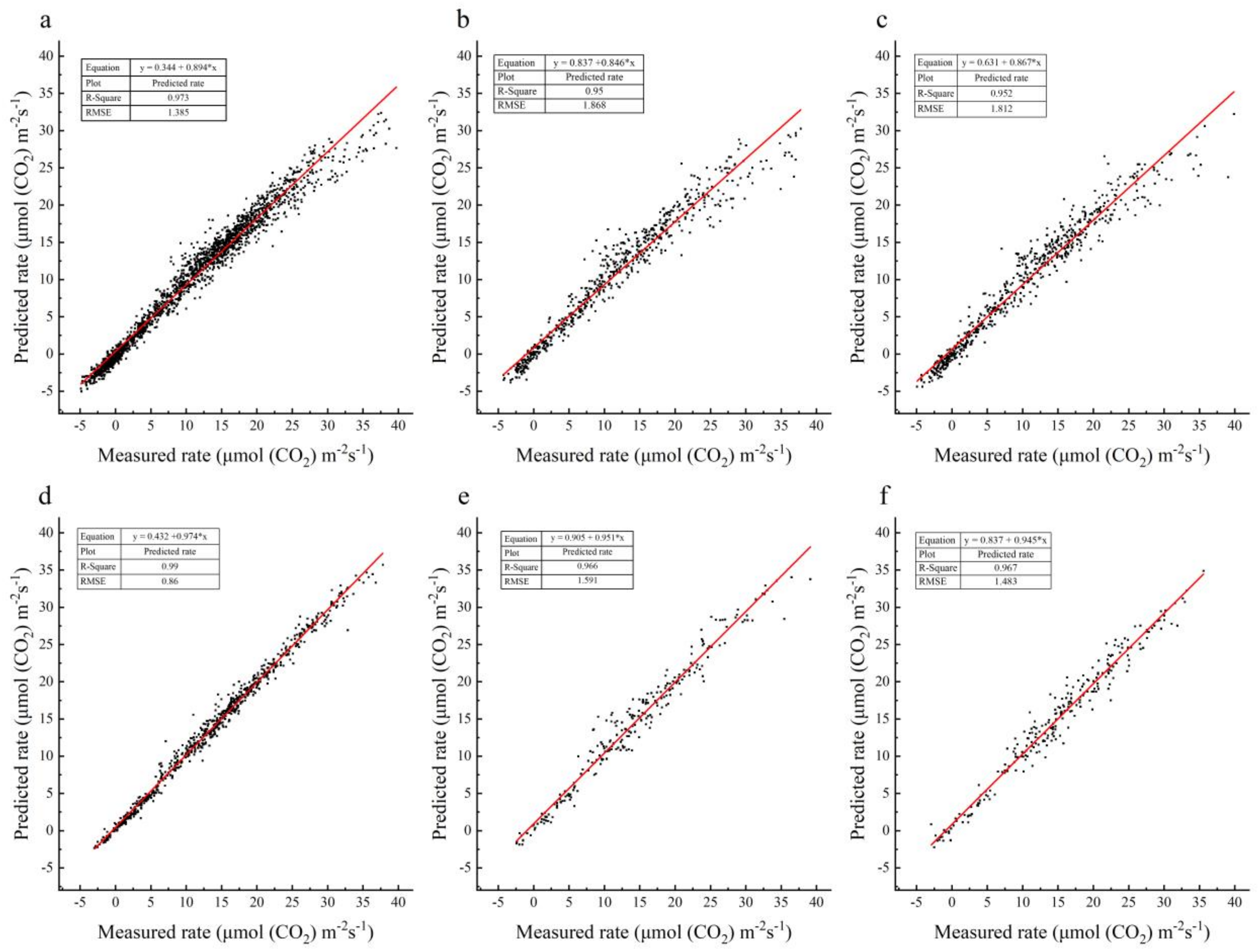
3.1. Performance of the Models

This article divided the dataset using five-fold cross-validation and used genetic algorithm (GA) and grid search technologies to optimize the hyperparameters of polynomial regression, KNN, GP, SVR, RF, Adaboost, GBDT, XGBoost, and NN models, and then found the upper limits of the fitting effect of each model for two photosynthesis datasets measured using air and 2% O₂, respectively.

Table 1. Fitting performance of different machine learning models.

Method	Model	Hyper-Parameters 1	Value	Dataset	EV	MAPE	RMSE	R2	Time-Consuming
Polynomial regression	Air based	degree	2	Validation set	0.905	1.093	2.974	0.905	25 ms
		interaction_only	FALSE
		include_bias	TRUE	Test set	0.899	1.010	2.947	0.899
	2% O2 based	degree	3	Validation set	0.937	0.443	2.236	0.937
		interaction_only	FALSE
		include_bias	TRUE	Test set	0.938	0.363	2.125	0.937
k-nearest neighbors (KNN)	Air based	n_neighbors	2	Validation set	0.919	0.714	2.815	0.915	356 ms
		weights	‘distance’
		algorithm	‘brute’
		leaf_size	40	Test set	0.912	0.698	2.770	0.910
		p	2
	2% O2 based	n_neighbors	2	Validation set	0.861	1.533	3.328	0.86
		weights	‘distance’
		algorithm	‘ball_tree’
		leaf_size	70	Test set	0.881	0.486	2.945	0.879
		p	2
Gaussian process (GP)	Air based	kernel	Rational Quadratic	Validation set	0.851	2.179	3.750	0.848	24.5 s
		length_scale	1.2
		alpha	1	Test set	0.859	2.317	3.477	0.859
	2% O2 based	kernel	Rationa lQuadratic	Validation set	0.906	1.302	2.729	0.906
		length_scale	1
		alpha	1.3	Test set	0.923	0.369	2.378	0.921
Support vector regression (SVR)	Air based	C	385.49	Validation set	0.954	0.525	2.083	0.953	17.2 s
		kernel	rbf	Test set	0.947	0.550	2.139	0.947
	2% O2 based	C	598.15	Validation set	0.924	0.746	2.454	0.924
		kernel	rbf	Test set	0.936	0.355	2.147	0.936
Random Forest (RF)	Air based	n_estimators	280	Validation set	0.962	0.366	1.894	0.961	945 ms
		criterion	‘mse’
		max_depth	24
		min_samples_split	6	Test set	0.961	0.370	1.835	0.961
		min_samples_leaf	3
		max_features	‘log2’
	2% O2 based	n_estimators	190	Validation set	0.955	0.480	1.894	0.955
		criterion	‘mse’
		max_depth	15
		min_samples_split	6	Test set	0.963	0.153	1.634	0.963
		min_samples_leaf	3
		max_features	‘auto’
Adaboost	Air based	loss	‘linear’	Validation set	0.869	1.391	3.485	0.869	295 ms
		n_estimators	154
		learning_rate	3.675	Test set	0.864	1.125	3.421	0.863
	2% O2 based	loss	‘linear’	Validation set	0.908	1.136	2.718	0.907
		n_estimators	88
		learning_rate	3.04	Test set	0.911	0.257	2.537	0.910
Gradient Boosting Decision Tree (GBDT)	Air based	loss	‘huber’	Validation set	0.959	0.400	1.949	0.959	705 ms
		learning_rate	0.24
		n_estimators	169
		subsample	0.84	Test set	0.960	0.409	1.843	0.960
		criterion	‘friedman_mse’
	2% O2 based	loss	‘ls’	Validation set	0.959	0.589	1.810	0.959
		learning_rate	0.38
		n_estimators	177
		subsample	0.66	Test set	0.959	0.260	1.732	0.958
		criterion	‘friedman_mse’
XGBoost	Air based	num_round	400	Validation set	0.970	0.334	1.667	0.970	779 ms
		obj	‘reg:linear’
		max_depth	5
		eta	0.08
		gamma	4	Test set	0.970	0.327	1.607	0.970
		alpha	4
		colsample_bytree	0.85
	2% O2 based	num_round	400	Validation set	0.971	0.271	1.523	0.971
		obj	‘reg:linear’
		max_depth	4
		eta	0.07
		gamma	0	Test set	0.970	0.181	1.469	0.970
		alpha	4
		colsample_bytree	0.9
Neural network (NN)	Air based	layers	4	Validation set	0.958	1.465	1.992	0.957	85.3 s
		each_layer_nodes	[20, 22, 19, 1]
		activation_function	‘sigmoid’
		optimizer	‘SGD’
		learning_rate	0.1	Test set	0.959	1.501	1.893	0.958
		momentum	0.8
		epochs	1000
	2% O2 based	layers	3	Validation set	0.924	0.862	2.450	0.924
		each_layer_nodes	[23, 8, 1]
		activation_function	‘sigmoid’
		optimizer	‘SGD’
		learning_rate	0.1	Test set	0.933	0.435	2.183	0.933
		momentum	0.8
		epochs	1000

¹ If the hyper-parameters of the model involve the selection of random seeds, they are all set to 0, and the other hyper-parameters use the default values if they are not listed.

shows the optimal hyperparameters for these models and the effectiveness of the four evaluation metrics (explained variance score, EV, mean absolute percentage error, MAPE, root mean square error, RMSE, coefficient of determination, R²) when using the holdout cross-validation divided datasets (60% for the training set, 20% for the validation set, and 20% for the test set). As can be seen from Table 1, for both datasets, the XGBoost models have the best performance in terms of prediction. The R² of all these models is above 0.85, which indicates that all these models have good fit and a substantial extent of explanation of the dependent variable by the independent variables, with RF, GBDT, XGBoost and NN (air based) models reaching above 0.95 and XGBoost being the best. It can be observed from this table that the values of EV and R² scores for each model are approximately the same, that is because their average error is almost zero. For the evaluation metric MAPE, the SVR model also performs better besides the three methods RF, GBDT, and XGBoost, while the other models have the value > 1, which means that these models have poor prediction performance when the photosynthesis value is low. The XGBoost model has the smallest RMSE value, and it suggests that the model has a small maximum error of prediction, but with a limited difference from GBDT and RF. Among these models, polynomial regression has the fastest modeling and solving speed of 25 ms. Although it has the worst results among all the models that were established, it still has a certain prediction accuracy. GP, SVR and NN were modeled slower, where the number of epochs was set to 1000 in order to improve the accuracy of the NN model, and the number of epochs can usually be reduced to decrease the time-consuming model training. Except for the three slower models, the training and prediction elapsed time of all the models is within 1000 ms. Therefore, the XGBoost model is the optimal model in terms of both prediction accuracy and time efficiency.

In particular, analyzing the XGBoost model in more detail (Figure 3), it is found that in most cases the predicted values are very close to the desired values. The accuracy of the photosynthesis model with the adverse effect of photorespiration decreases when measured values are higher, especially and most significantly in the validation set. Contrastingly, for the model of photosynthesis without the effect of photorespiration, there is no such problem.

NN are increasingly used, and the interpretability of the models built by NN is given more importance [51]. However, the interpretability of NN models is relatively poor. In many studies, it was shown that neural networks seem to have stronger predictive capability [52]. However, for the light respiration model discussed in this study, not only did it require a lot of computing power and time to build the light respiration model using the NN approach, but it also required more time cost to make predictions (108.5 times more than the model built using XGBoost), and above all the model performed poorly (R² of 0.958 and 0.933 for the test set, which lower than 0.970 and 0.970 in XGBoost model). From these three aspects, the XGBoost algorithm developed based on decision trees is more advantageous. The XGBoost algorithm has been used to some extent in many fields [53,54], and there are also an increasing number of algorithms that use this idea. Many weak learner instances of the algorithm are being pooled (via boosting, bagging, etc.) together to create a strong ensemble learner, with some success [55,56]. Thus, researchers need to pay more attention to integration learning.

3.2. Potential for Model Performance Enhancing

Data and features determine the upper limit of machine learning, so both are crucial. Although the data provided for the building of this model is large enough (about 4000+ datasets), for the dataset obtained from the experimental measurements, there must be a range of features that it failed to cover, i.e., these samples were not fully representative of the overall population. It required a high generalization ability of the model. Especially, this study integrated the two machine learning models in an arithmetic operation rather than starting from the mechanics of the model. Thus, the generalization error of the model was also presented in the prediction results of photorespiration in the same way as arithmetic operations, making some predictions out of the theoretical range. This can only be solved by providing more data to the model.

The number of features is not always the more the better. In this study, the filtering method was used to select features for the datasets. The features were first filtered by the variances of themselves. If the variance of a feature is small, it means that the sample has less variation in this feature, which means that the feature is less useful for differentiating the sample. After calculating the variance of each feature, it was found that the variance of cucumber growth stage was the smallest at 0.21, followed by plant location (X, Y) in the greenhouse at 0.61 and 0.65, respectively, and the variance of all other features was larger (value > 5). Therefore, the growth stage can be excluded. If it is excluded and the XGBoost model is reconstructed, the model performance is shown in

Table 2. Fitting performance of alternative models.

Method	Model	Hyper-Parameters 1	Value	Dataset	EV	MAPE	RMSE	R2	Time-Consuming
XGBoost	air based	num_round	1000	Validation set	0.975	0.254	1.527	0.975	1.62 s
		obj	‘reg:linear’
		max_depth	6
		eta	0.15
		lambda	3	Test set	0.976	0.365	1.439	0.976
		alpha	0
		colsample_bylevel	0.4
		colsample_bynode	1
	2% O2 based	num_round	275	Validation set	0.968	0.255	1.584	0.968
		obj	‘reg:linear’
		max_depth	4
		eta	0.07
		lambda	0.9	Test set	0.970	0.199	1.483	0.969
		alpha	4
		colsample_bylevel	1
		colsample_bynode	0.5

¹ If the hyper-parameters of the model involve the selection of random seeds, they are all set to 0. The other hyper-parameters use the default values if they are not listed.

. The comparison between Table 2 and Table 1 shows that the new has limited improvement for the dataset measured using air and is rather worse for the dataset measured using 2% O₂. It means that the exclusion of this feature has little effect on the model. Next, the correlation between features was checked. If two variables are highly correlated among themselves, they provide redundant information about the target. Essentially, an accurate prediction of the target can be made using only one of the redundant variables. In addition, removing redundant variables can help reduce dimensionality and damp out noise. Figure 4 represents the absence of a strong association between any two features (correlation coefficient < −0.5 or >0.5).

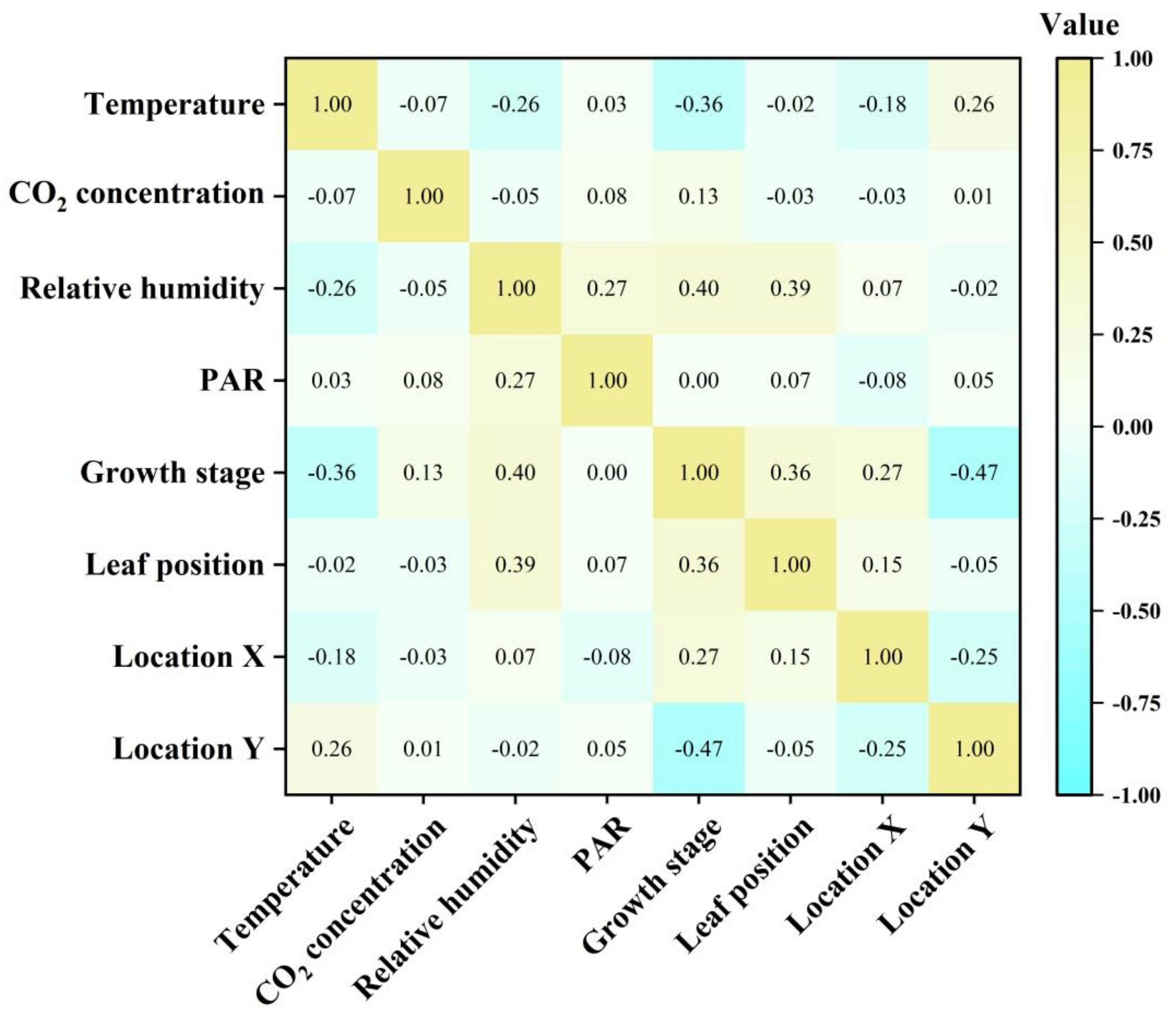
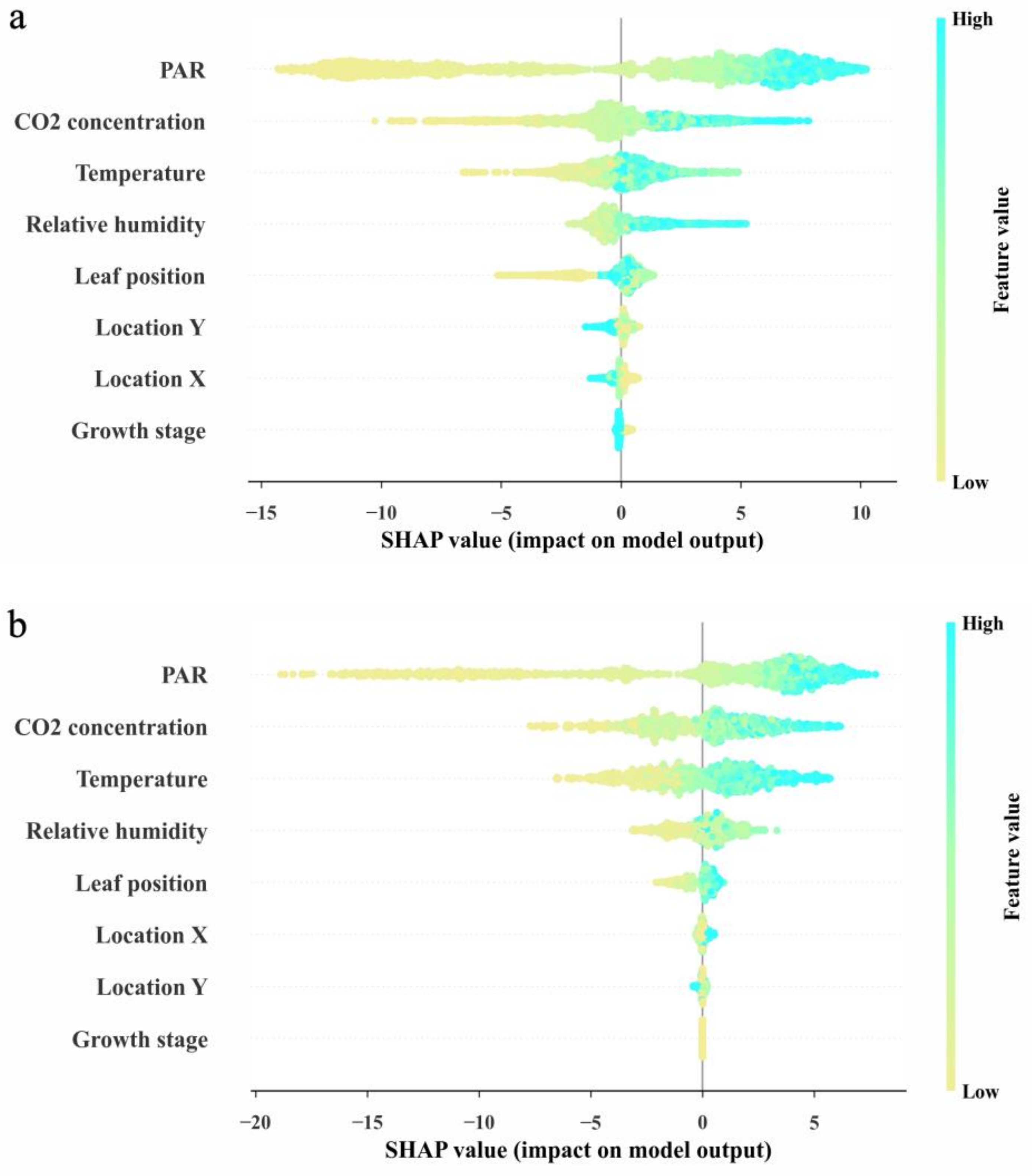
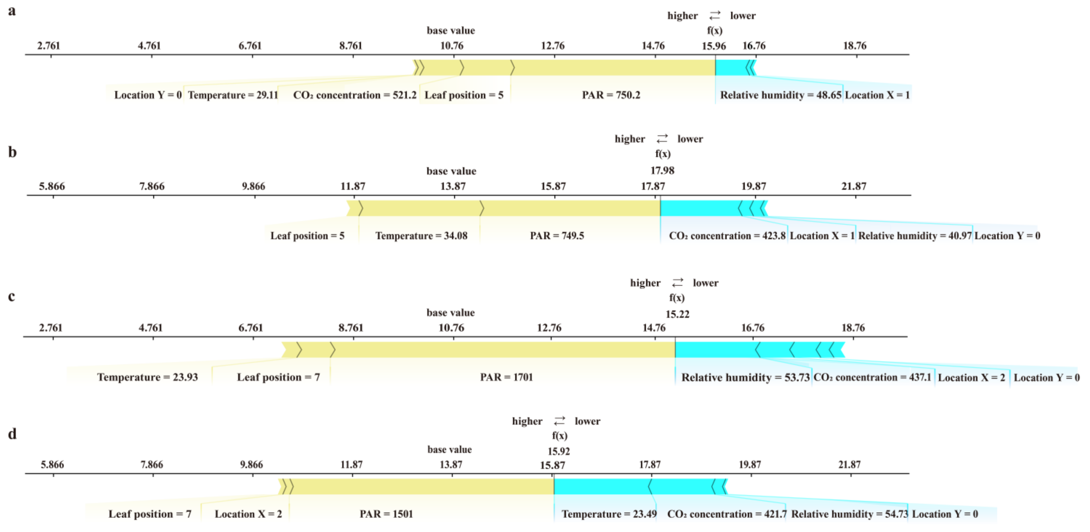
3.3. Interpretability of the Model and the Main Factors Affecting the Photorespiration

The XGBoost method is based on the gradient boosting tree and has shown high accuracy in this study, but the interpretability is not clear enough and is often referred to as a “black box” model. Therefore, the importance ranking of feature values (Figure 5) can only give a general overview of each feature’s importance and cannot determine the relationship between the features and the final prediction results.

Some researchers have used the SHapley Additive explanation (SHAP), which originates from cooperative game theory, to explore the influence of each feature of the model [57,58]. Figure 6 shows the SHAP values that order features based on their importance to photosynthesis rate (a) with an adverse effect of photorespiration and (b) without the effect. The strength order of influence of the two groups of features is almost the same, except for their position in the greenhouse. PAR is a very important feature and is positively correlated with photosynthesis rate most of the time. However, when the relationship is negative, the influence is significantly stronger. Additionally, PAR is less influential in regular photosynthesis. In contrast, it is more influential when photorespiration is excluded. It is implied that PAR is less important for the predicted photorespiration values obtained by subtracting the two predictions. Humidity is mostly negatively correlated in Figure 6a, while the importance is relatively small, but when it shows a positive correlation, the importance became large, reaching almost half of PAR at the highest. The leaf position, on the other hand, behaves as just the opposite of humidity. In the prediction of photosynthetic rate without the effect of photorespiration (Figure 6b), the influence of humidity is lower overall, and the positive and negative correlations are more even; leaf position followed the same trend as the results in Figure 6a. Growth stage is the least important of the two models.

Two data with approximately the same feature values from each of the two models’ training sets are selected for visual analysis of the feature importance, as shown in Figure 7a–d. The features positively correlated with the prediction results are shown in red, and the negatively correlated features are shown in blue, and the effects of these features are plotted against each other to obtain the prediction results. In all plots, PAR has the largest positive effect. The difference between Figure 7a,b is that CO₂ concentration and Location Y, which have a positive effect in (a), are negative effects in (b). The difference between Figure 7c,d is that Temperature, which has a weaker positive effect in (c), plays a stronger negative effect in (d), and Relative Humidity, which has a larger negative effect in (c), has a smaller effect in (d). In conclusion, it indicates that the importance of each feature in the photorespiration model differs significantly from that in the photosynthesis model.

Although the above showed partial trends of individual features, the SHAP analysis based solely on themselves was still not clear enough since the photorespiration model is obtained by subtracting two original XGBoost models. Therefore, models constructed by the polynomial regression approach, as a most interpretable model, were necessary to be analyzed.

Although the polynomial regression performed weakly in these models, the R² of the models still achieved about 0.9 (Table 1). According to the operational logic of Equation (5), the two models built using polynomial regression can be written with expressions in analytic form. The maximum term in the polynomial is a three-degree term. Thus, photorespiration model can be easily expressed in equations. The meaning and coefficients of each term of the photosynthesis model and photorespiration model are shown in

Table 3. Meaning and coefficients of terms of the photosynthesis model and photorespiration model.

Photosynthesis Model		Photorespiration Model
Term 1	Coefficient	Term 2	Coefficient
PAR	8.221	Leaf position × Location Y	18.015
CO2 concentration	3.122	Temperature	13.639
Location Y	2.089	Temperature × Growth stage 2	13.418
Leaf position	1.503	Location X	12.691
Relative humidity	1.500	Leaf position × Location X × Location Y	12.439
Temperature × Growth stage	1.314	Growth stage 2 × Location X	12.349
CO2 concentration × PAR	1.280	Temperature × Location X × Location Y	10.540
Temperature × PAR	1.190	Relative humidity × Location X × Location Y	9.122
…	…	…	…
…	…	…	…
…	…	…	…
CO2 concentration × Growth stage	−0.485	Temperature × Location X	−11.009
Temperature 2	−0.505	Leaf position × Location X	−11.591
PAR × Location X	−0.737	Growth stage × Leaf position × Location X	−11.620
Growth stage × Location Y	−0.892	Location X × Location Y 2	−14.085
Growth stage × Location X	−1.089	Leaf position	−15.735
Relative humidity × Growth stage	−1.094	Location X 2 × Plant Location Y	−15.925
Location Y 2	−1.266	Growth stage 2 × Plant Location Y	−18.780
PAR 2	−3.704	Location Y	−20.869

¹ There are 45 items in the photosynthesis model, and the 16 items with the highest absolute values of each coefficient are selected in the table; ² There are 169 items in the photorespiration model, and the 16 items with the highest absolute values of each coefficient are selected in the table.

. For the photosynthesis model, PAR, CO₂ concentration, Location Y in greenhouse (which mainly affects the microclimate), leaf position, and relative humidity (absolute value of coefficient > 1.5) were the most important features. The coefficients of light and light² had the largest absolute values, 8.221 and −3.704, respectively. The second was the CO₂ concentration. These results are consistent with the general understanding of photosynthesis. In contrast, for the predictive model of photorespiration, it found that leaf position, growth stage, location in greenhouse, temperature, relative humidity, and their mutual products (absolute value of coefficient >9) were important features, while the absolute coefficient of PAR was not as high. This suggests that when studying photorespiration, more attention needs to be paid to the growth stage, leaf position, temperature, and relative humidity, rather than PAR.

3.4. Soft Sensors and Ability to Promote

Some studies have claimed that these predictive models can be applied as soft sensors in greenhouses [59,60]. This significantly reduces the cost required to configure the sensors. However, this sensor-like process requires a model that is sufficiently accurate and has a very high generalization ability. The model establishment for the photorespiration of cucumber makes it happen that the leaf photorespiration rate can be predicted through the basic meteorological parameters around the leaf with high simulation accuracy and obtainable parameters. Therefore, the model developed in this study can be applied as a soft sensor. It can be a useful exploration of research on photorespiration rate simulation. Machine-learning-simulated photorespiration involves statistical models based on datasets. In this study, measurements from two production seasons of cucumber were used in order to be more accurate. In fact, using the method provided in this study, only measurements from one production season of a certain crop are needed to model crop photorespiration with high accuracy. It means that the model can be easily extended, promoted and applied to other plants.

4. Conclusions

This study compared the performance of several machine learning models to predict photorespiration rate in cucumber leaves. The photorespiration rate was expressed as the difference between the photosynthetic rate at 2% O₂ and 21% O₂ concentrations. For this purpose, air temperature, relative humidity, CO₂ concentration, PAR measurements near the leaves, crop growth period, leaf position, and plant location in the greenhouse were used as input variables to the models, and photosynthetic rates measured using air and 2% O₂, respectively, were used as output variables. Additionally, the advantages and disadvantages of the two models built using different machine learning methods were tested. It was observed that the XGBoost models had the best generalization ability and took less time, where the R² of the test set for both models with air and 2% oxygen measurements was 0.970. The importance of features was also discussed. It was found that PAR and CO₂ concentration have a greater effect on the photosynthetic rate itself, but temperature and relative humidity are more significant for photorespiration. The model established in this study performed well, with high accuracy and generalization ability. In addition, the model can be used as a soft sensor. Additionally, it has a certain ability to promote to other plants.

References

1. Liang, Y.; Kang, C.; Kaiser, E.; Kuang, Y.; Yang, Q.; Li, T. Red/Blue Light Ratios Induce Morphology and Physiology Alterations Differently in Cucumber and Tomato. Sci. Hortic. 2021, 281, 109995. [Google Scholar] [CrossRef]
2. Li, Y.; Liu, C.; Shi, Q.; Yang, F.; Wei, M. Mixed Red and Blue Light Promotes Ripening and Improves Quality of Tomato Fruit by Influencing Melatonin Content. Environ. Exp. Bot. 2021, 185, 104407. [Google Scholar] [CrossRef]
3. Takahashi, S.; Murata, N. Glycerate-3-Phosphate, Produced by CO2 Fixation in the Calvin Cycle, Is Critical for the Synthesis of the D1 Protein of Photosystem II. Biochim. Biophys. Acta Bioenergy 2006, 1757, 198–205. [Google Scholar] [CrossRef] [Green Version]
4. Kimura, K.; Yasutake, D.; Koikawa, K.; Kitano, M. Spatiotemporal Variability of Leaf Photosynthesis and Its Linkage with Microclimates across an Environment-Controlled Greenhouse. Biosyst. Eng. 2020, 195, 97–115. [Google Scholar] [CrossRef]
5. Fara, S.J.; Teixeira Delazari, F.; Silva Gomes, R.; Araújo, W.L.; da Silva, D.J.H. Stomata Opening and Productiveness Response of Fresh Market Tomato under Different Irrigation Intervals. Sci. Hortic. 2019, 255, 86–95. [Google Scholar] [CrossRef]
6. Flügel, F.; Timm, S.; Arrivault, S.; Florian, A.; Stitt, M.; Fernie, A.R.; Bauwe, H. The Photorespiratory Metabolite 2-Phosphoglycolate Regulates Photosynthesis and Starch Accumulation in Arabidopsis. Plant Cell 2017, 29, 2537–2551. [Google Scholar] [CrossRef] [Green Version]
7. De FC Carvalho, J.; Madgwick, P.J.; Powers, S.J.; Keys, A.J.; Lea, P.J.; Parry, M.A.J. An Engineered Pathway for Glyoxylate Metabolism in Tobacco Plants Aimed to Avoid the Release of Ammonia in Photorespiration. BMC Biotechnol. 2011, 11, 111. [Google Scholar] [CrossRef] [Green Version]
8. López-Calcagno, P.E.; Fisk, S.; Brown, K.L.; Bull, S.E.; South, P.F.; Raines, C.A. Overexpressing the H-Protein of the Glycine Cleavage System Increases Biomass Yield in Glasshouse and Field-Grown Transgenic Tobacco Plants. Plant Biotechnol. J. 2019, 17, 141–151. [Google Scholar] [CrossRef]
9. Rae, B.D.; Long, B.M.; Förster, B.; Nguyen, N.D.; Velanis, C.N.; Atkinson, N.; Hee, W.Y.; Mukherjee, B.; Price, G.D.; McCormick, A.J. Progress and Challenges of Engineering a Biophysical CO2-Concentrating Mechanism into Higher Plants. J. Exp. Bot. 2017, 68, 3717–3737. [Google Scholar] [CrossRef]
10. South, P.F.; Cavanagh, A.P.; Liu, H.W.; Ort, D.R. Synthetic Glycolate Metabolism Pathways Stimulate Crop Growth and Productivity in the Field. Science 2019, 363, eaat9077. [Google Scholar] [CrossRef] [Green Version]
11. Zhu, X.G.; Portis, A.R.; Long, S.P. Would Transformation of C3 Crop Plants with Foreign Rubisco Increase Productivity? A Computational Analysis Extrapolating from Kinetic Properties to Canopy Photosynthesis. Plant Cell Environ. 2004, 27, 155–165. [Google Scholar] [CrossRef]
12. Galmés, J.; Hermida-Carrera, C.; Laanisto, L.; Niinemets, Ü. A Compendium of Temperature Responses of Rubisco Kinetic Traits: Variability among and within Photosynthetic Groups and Impacts on Photosynthesis Modeling. J. Exp. Bot. 2016, 67, 5067–5091. [Google Scholar] [CrossRef] [Green Version]
13. Hermida-Carrera, C.; Kapralov, M.V.; Galmés, J. Rubisco Catalytic Properties and Temperature Response in Crops. Plant Physiol. 2016, 171, 2549–2561. [Google Scholar] [CrossRef] [Green Version]
14. Busch, F.A. Photorespiration in the Context of Rubisco Biochemistry, CO2 Diffusion and Metabolism. Plant J. 2020, 101, 919–939. [Google Scholar] [CrossRef] [Green Version]
15. Huang, W.; Hu, H.; Zhang, S.-B. Photorespiration Plays an Important Role in the Regulation of Photosynthetic Electron Flow under Fluctuating Light in Tobacco Plants Grown under Full Sunlight. Front. Plant Sci. 2015, 6, 621. [Google Scholar] [CrossRef] [Green Version]
16. Kangasjarvi, S.; Neukermans, J.; Li, S.; Aro, E.M.; Noctor, G. Photosynthesis, Photorespiration, and Light Signalling in Defence Responses. J. Exp. Bot. 2012, 63, 1619–1636. [Google Scholar] [CrossRef] [Green Version]
17. Lin, Z.; Peng, C.; Sun, Z.; Lin, G. Effect of Light Intensity on Partitioning of Photosynthetic Electron Transport to Photorespiration in Four Subtropical Forest Plants. Sci. China Ser. C Life Sci. 2000, 43, 347–354. [Google Scholar] [CrossRef]
18. Ye, Z.P. A New Model for Relationship between Irradiance and the Rate of Photosynthesis in Oryza Sativa. Photosynthetica 2007, 45, 637–640. [Google Scholar] [CrossRef]
19. Ye, Z.P.; Duan, S.H.; Chen, X.M.; Duan, H.L.; Gao, C.P.; Kang, H.J.; An, T.; Zhou, S.X. Quantifying Light Response of Photosynthesis: Addressing the Long-Standing Limitations of Non-Rectangular Hyperbolic Model. Photosynthetica 2021, 59, 185–191. [Google Scholar] [CrossRef]
20. Lanoue, J.; Leonardos, E.D.; Grodzinski, B. Effects of Light Quality and Intensity on Diurnal Patterns and Rates of Photo-Assimilate Translocation and Transpiration in Tomato Leaves. Front. Plant Sci. 2018, 9, 756. [Google Scholar] [CrossRef] [Green Version]
21. Farquhar, G.D.; von Caemmerer, S.; Berry, J.A. A Biochemical Model of Photosynthetic CO2 Assimilation in Leaves of C 3 Species. Planta 1980, 149, 78–90. [Google Scholar] [CrossRef] [PubMed] [Green Version]
22. Gu, L.; Pallardy, S.G.; Tu, K.; Law, B.E.; Wullschleger, S.D. Reliable Estimation of Biochemical Parameters from C3 Leaf Photosynthesis-Intercellular Carbon Dioxide Response Curves. Plant Cell Environ. 2010, 33, 1852–1874. [Google Scholar] [CrossRef]
23. Miranda-Apodaca, J.; Marcos-Barbero, E.L.; Morcuende, R.; Arellano, J.B. Surfing the Hyperbola Equations of the Steady-State Farquhar–von Caemmerer–Berry C3 Leaf Photosynthesis Model: What Can a Theoretical Analysis of Their Oblique Asymptotes and Transition Points Tell Us? Bull. Math. Biol. 2020, 82, 3. [Google Scholar] [CrossRef] [Green Version]
24. Moualeu-Ngangue, D.P.; Chen, T.-W.; Stützel, H. A New Method to Estimate Photosynthetic Parameters through Net Assimilation Rate–Intercellular Space CO2 Concentration (A–C i) Curve and Chlorophyll Fluorescence Measurements. New Phytol. 2017, 213, 1543–1554. [Google Scholar] [CrossRef]
25. Coursolle, C.; Otis Prud Homme, G.; Lamothe, M.; Isabel, N. Measuring Rapid A–Ci Curves in Boreal Conifers: Black Spruce and Balsam Fir. Front. Plant Sci. 2019, 10, 1276. [Google Scholar] [CrossRef] [Green Version]
26. Han, T.; Zhu, G.; Ma, J.; Wang, S.; Zhang, K.; Liu, X.; Ma, T.; Shang, S.; Huang, C. Sensitivity Analysis and Estimation Using a Hierarchical Bayesian Method for the Parameters of the FvCB Biochemical Photosynthetic Model. Photosynth. Res. 2020, 143, 45–66. [Google Scholar] [CrossRef]
27. Wang, Q.; Chun, J.; Fleisher, D.; Reddy, V.; Timlin, D.; Resop, J. Parameter Estimation of the Farquhar—von Caemmerer—Berry Biochemical Model from Photosynthetic Carbon Dioxide Response Curves. Sustainability 2017, 9, 1288. [Google Scholar] [CrossRef] [Green Version]
28. Xiong, D.; Liu, X.; Liu, L.; Douthe, C.; Li, Y.; Peng, S.; Huang, J. Rapid Responses of Mesophyll Conductance to Changes of CO2 Concentration, Temperature and Irradiance Are Affected by N Supplements in Rice. Plant Cell Environ. 2015, 38, 2541–2550. [Google Scholar] [CrossRef]
29. Kaiser, E.; Morales, A.; Harbinson, J.; Kromdijk, J.; Heuvelink, E.; Marcelis, L.F.M. Dynamic Photosynthesis in Different Environmental Conditions. J. Exp. Bot. 2015, 66, 2415–2426. [Google Scholar] [CrossRef] [Green Version]
30. Morales, A.; Kaiser, E.; Yin, X.; Harbinson, J.; Molenaar, J.; Driever, S.M.; Struik, P.C. Dynamic Modelling of Limitations on Improving Leaf CO2 Assimilation under Fluctuating Irradiance. Plant Cell Environ. 2018, 41, 589–604. [Google Scholar] [CrossRef] [Green Version]
31. Li, P.-P.; Wang, J.-Z.; Chen, X.; Liu, W.-H. Studies on Photosynthesis Model of Mini-Cucumber Leaf in Greenhouse. In Crop Modeling and Decision Support; Springer: Berlin, Germany, 2009; pp. 24–29. ISBN1 978-3-642-01131-3. ISBN2 978-3-642-01132-0. [Google Scholar]
32. Peri, P.L.; Arena, M.; Martínez Pastur, G.; Lencinas, M.V. Photosynthetic Response to Different Light Intensities, Water Status and Leaf Age of Two Berberis Species (Berberidaceae) of Patagonian Steppe, Argentina. J. Arid. Environ. 2011, 75, 1218–1222. [Google Scholar] [CrossRef]
33. Zhang, J.; Wang, S. Simulation of the Canopy Photosynthesis Model of Greenhouse Tomato. Procedia Eng. 2011, 16, 632–639. [Google Scholar] [CrossRef] [Green Version]
34. Goltsev, V.; Zaharieva, I.; Chernev, P.; Kouzmanova, M.; Kalaji, H.M.; Yordanov, I.; Krasteva, V.; Alexandrov, V.; Stefanov, D.; Allakhverdiev, S.I.; et al. Drought-Induced Modifications of Photosynthetic Electron Transport in Intact Leaves: Analysis and Use of Neural Networks as a Tool for a Rapid Non-Invasive Estimation. Biochim. Biophys. Acta Bioenergy 2012, 1817, 1490–1498. [Google Scholar] [CrossRef] [Green Version]
35. Heckmann, D.; Schlüter, U.; Weber, A.P.M. Machine Learning Techniques for Predicting Crop Photosynthetic Capacity from Leaf Reflectance Spectra. Mol. Plant 2017, 10, 878–890. [Google Scholar] [CrossRef] [Green Version]
36. Jian, Y.; Xinying, L.; Man, Z.; Han, L. Photosynthetic Rate Prediction of Tomato Plant Population Based on PSO and GA. IFAC-PapersOnLine 2018, 51, 61–66. [Google Scholar] [CrossRef]
37. Zhang, X.Y.; Huang, Z.; Su, X.; Siu, A.; Song, Y.; Zhang, D.; Fang, Q. Machine Learning Models for Net Photosynthetic Rate Prediction Using Poplar Leaf Phenotype Data. PLoS ONE 2020, 15, e0228645. [Google Scholar] [CrossRef] [Green Version]
38. Dusenge, M.E.; Duarte, A.G.; Way, D.A. Plant Carbon Metabolism and Climate Change: Elevated CO2 and Temperature Impacts on Photosynthesis, Photorespiration and Respiration. New Phytol. 2019, 221, 32–49. [Google Scholar] [CrossRef] [Green Version]
39. Huang, S.; Jacoby, R.P.; Shingaki-Wells, R.N.; Li, L.; Millar, A.H. Differential Induction of Mitochondrial Machinery by Light Intensity Correlates with Changes in Respiratory Metabolism and Photorespiration in Rice Leaves. New Phytol. 2013, 198, 103–115. [Google Scholar] [CrossRef] [PubMed] [Green Version]
40. Slot, M.; Garcia, M.N.; Winter, K. Temperature Response of CO2 Exchange in Three Tropical Tree Species. Funct. Plant Biol. 2016, 43, 468–478. [Google Scholar] [CrossRef]
41. Walker, B.J.; Orr, D.J.; Carmo-Silva, E.; Parry, M.A.J.; Bernacchi, C.J.; Ort, D.R. Uncertainty in Measurements of the Photorespiratory CO2 Compensation Point and Its Impact on Models of Leaf Photosynthesis. Photosynth. Res. 2017, 132, 245–255. [Google Scholar] [CrossRef]
42. Busch, F.A. Current Methods for Estimating the Rate of Photorespiration in Leaves. Plant Biol. 2013, 15, 648–655. [Google Scholar] [CrossRef]
43. Shalaby, T.A.; Abd-Alkarim, E.; El-Aidy, F.; Hamed, E.-S.; Sharaf-Eldin, M.; Taha, N.; El-Ramady, H.; Bayoumi, Y.; dos Reis, A.R. Nano-Selenium, Silicon and H2O2 Boost Growth and Productivity of Cucumber under Combined Salinity and Heat Stress. Ecotoxicol. Environ. Saf. 2021, 212, 111962. [Google Scholar] [CrossRef]
44. Tang, F.; Ishwaran, H. Random Forest Missing Data Algorithms. Stat. Anal. Data Min. 2017, 10, 363–377. [Google Scholar] [CrossRef]
45. Breiman, L. Random Forests. Mach. Learn. 2001, 45, 5–32. [Google Scholar] [CrossRef] [Green Version]
46. Elavarasan, D.; Vincent, D.R.; Sharma, V.; Zomaya, A.Y.; Srinivasan, K. Forecasting Yield by Integrating Agrarian Factors and Machine Learning Models: A Survey. Comput. Electron. Agric. 2018, 155, 257–282. [Google Scholar] [CrossRef]
47. Goh, A.H.A.; Ali, Z.; Nor, N.M.; Baharum, A.; Ahmad, W.M.A.W. A Quadratic Regression Modelling on Paddy Production in the Area of Perlis. AIP Conf. Proc. 2017, 1870, 060015. [Google Scholar] [CrossRef]
48. Ebrahimi, M.A.; Khoshtaghaza, M.H.; Minaei, S.; Jamshidi, B. Vision-Based Pest Detection Based on SVM Classification Method. Comput. Electron. Agric. 2017, 137, 52–58. [Google Scholar] [CrossRef]
49. Freund, Y.; Schapire, R.E. A Decision-Theoretic Generalization of On-Line Learning and an Application to Boosting. J. Comput. Syst. Sci. 1997, 55, 119–139. [Google Scholar] [CrossRef] [Green Version]
50. Chen, T.; Guestrin, C. XGBoost: A Scalable Tree Boosting System. In Proceedings of the KDD ’16: 22nd ACM SIGKDD International Conference on Knowledge Discovery and Data Mining 2016, San Francisco, CA, USA, 13–17 August 2016; pp. 785–794. [Google Scholar] [CrossRef] [Green Version]
51. Gilpin, L.H.; Bau, D.; Yuan, B.Z.; Bajwa, A.; Specter, M.; Kagal, L. Explaining Explanations: An Overview of Interpretability of Machine Learning. In Proceedings of the 2018 IEEE 5th International Conference on Data Science and Advanced Analytics (DSAA), Turin, Italy, 1–4 October 2018; pp. 80–89. [Google Scholar]
52. Liakos, K.G.; Busato, P.; Moshou, D.; Pearson, S.; Bochtis, D. Machine Learning in Agriculture: A Review. Sensors 2018, 18, 2674. [Google Scholar] [CrossRef] [Green Version]
53. Cardoso, J.; Gloria, A.; Sebastiao, P. Improve Irrigation Timing Decision for Agriculture Using Real Time Data and Machine Learning. In Proceedings of the 2020 International Conference on Data Analytics for Business and Industry: Way Towards a Sustainable Economy (ICDABI), Sakheer, Bahrain, 26–27 October 2020; pp. 1–5. [Google Scholar]
54. Elavarasan, D.; Vincent, D.R. Reinforced XGBoost Machine Learning Model for Sustainable Intelligent Agrarian Applications. J. Intell. Fuzzy Syst. 2020, 39, 7605–7620. [Google Scholar] [CrossRef]
55. Conţiu, Ş.; Groza, A. Improving Remote Sensing Crop Classification by Argumentation-Based Conflict Resolution in Ensemble Learning. Expert Syst. Appl. 2016, 64, 269–286. [Google Scholar] [CrossRef]
56. Wu, T.; Zhang, W.; Jiao, X.; Guo, W.; Alhaj Hamoud, Y. Evaluation of Stacking and Blending Ensemble Learning Methods for Estimating Daily Reference Evapotranspiration. Comput. Electron. Agric. 2021, 184, 106039. [Google Scholar] [CrossRef]
57. Bi, Y.; Xiang, D.; Ge, Z.; Li, F.; Jia, C.; Song, J. An Interpretable Prediction Model for Identifying N7-Methylguanosine Sites Based on XGBoost and SHAP. Mol. Ther. Nucleic Acids 2020, 22, 362–372. [Google Scholar] [CrossRef]
58. Lundberg, S.M.; Lee, S.I. A Unified Approach to Interpreting Model Predictions. In Proceedings of the NIPS’17: 31st International Conference on Neural Information Processing Systems, Long Beach, CA, USA, 4–9 December 2017; Curran Associates Inc.: Long Beach, CA, USA, 2017; Volume 2017, pp. 4768–4777. [Google Scholar]
59. Jung, D.H.; Kim, H.S.; Jhin, C.; Kim, H.J.; Park, S.H. Time-Serial Analysis of Deep Neural Network Models for Prediction of Climatic Conditions inside a Greenhouse. Comput. Electron. Agric. 2020, 173, 105402. [Google Scholar] [CrossRef]
60. Liu, T.; Yuan, Q.Y.; Wang, Y.G. Prediction Model of Photosynthetic Rate Based on Sopso-Lssvm for Regulation of Greenhouse Light Environment. Eng. Lett. 2021, 29, 297–301. [Google Scholar]
Figure 1. Scenes and a sketch of the experiment field and instruments. (a) Seedling stages of the plants. (b) Instrument arrangement for measuring photosynthesis. (c) Instrument arrangement for measuring photorespiration. (d) A sketch of the defined Cartesian coordinate greenhouse floor plane.
Horticulturae 07 00207 g001
Figure 2. Distribution plots of the dataset. Temperature (a), CO2 concentration (b), relative humidity (c), PAR (d) values for measurements with air and temperature (e), CO2 concentration (f), relative humidity (g), PAR (h) values for measurements with 2% O2 showing lower (25th percentile − 1.5 × (75th quantile − 25th quantile)) and upper (75th percentile + 1.5 × (75th quantile − 25th quantile)) limits, 25th − 75th percentile (box) and median (horizontal line).
Horticulturae 07 00207 g002aHorticulturae 07 00207 g002b
Figure 3. Measured and predicted rate in the XGBoost model. (a) Scatter plot in training set with the effect of photorespiration. (b) Scatter plot in validation set with the effect of photorespiration. (c) Scatter plot in test set with the effect of photorespiration. (d) Scatter plot in training set without the effect of photorespiration. (e) Scatter plot in validation set without the effect of photorespiration. (f) Scatter plot in test set without the effect of photorespiration.
Horticulturae 07 00207 g003
Figure 4. Spearman correlation heat map with correlation coefficient based on the photosynthesis datasets measured using air.
Horticulturae 07 00207 g004
Figure 5. Feature importance of the models. (a) The model with the negative effect of photorespiration; (b) the model without the effect.
Horticulturae 07 00207 g005
Figure 6. SHAP summary plot. (a) is the model with the negative effect of photorespiration; (b) is the model without the effect of photorespiration.
Horticulturae 07 00207 g006
Figure 7. SHAP force plot. The feature values of (a,b) are approximately the same, with the feature value of (a) coming from the photosynthesis model with the effect of photorespiration and the feature value of (b) coming from the photosynthesis model without the effect of photorespiration; the feature values of (c,d) are approximately the same, with the feature value of (c) coming from the photosynthesis model with the effect of photorespiration and the feature value of (d) coming from the photosynthesis model without the effect of photorespiration.
Horticulturae 07 00207 g007