Effective Analysis of Interactive Effects with Non-Normal Data Using the Aligned Rank Transform, ARTool and SAS^® University Edition

Abstract

Most statistical techniques commonly used in horticultural research are parametric tests that are valid only for normal data with homogeneous variances. While parametric tests are robust when the data ‘slightly’ deviate from normality, a significant departure from normality leads to reduced power and the probability of a type I error increases. Transformations often used to normalize non-normal data can be time consuming, cumbersome and confusing and common non-parametric tests are not appropriate for evaluating interactive effects common in horticultural research. The aligned rank transformation allows non-parametric testing for interactions and main effects using standard ANOVA techniques. This has not been widely adapted due to its rigorous mathematical nature, however, a downloadable (ARTool) is now available, which performs the math needed for the transformation. This study provides step-by-step instructions for integrating ARTool with the free edition of SAS (SAS University Edition) in an easily employed method for testing normality, transforming data with aligned ranks, and analysing data using standard ANOVAs.

1. Introduction

The statistical methods used for data analysis of many horticultural studies are often subject to controversy during the review process. Researchers frequently use familiar techniques even though they may not be appropriate or valid. Many of the statistical techniques most commonly used in horticultural research such as the analysis of variance (ANOVA), t-tests, and linear regression, are parametric techniques that are valid only if the data in the analysis are normally and independently distributed with µ = 0 and common variance, σ², i.e., ‘normal data with homogeneous variances’ [1,2,3]. Tests for normality are available in computer statistical packages such as SAS, Stata, Minitab and R, yet this step is often overlooked during data analysis. While parametric tests are robust when the data ‘slightly’ deviate from normality, a significant departure can lead to incorrect conclusions. When parametric procedures are used on non-normal data, power (the probability of detecting a treatment effect when it does in fact exist) is greatly reduced and the probability of a type I error (declaring a significant treatment effect when there in fact is none) greatly increases [3].

When data is not normal, parametric techniques are not valid, thus, data are often transformed using one of many techniques. If the transformed data is normal when tested, subjecting the transformed data to a parametric analysis is valid. If the transformed data are not normal after transformation, a different transformation is used on the original data until a suitable transformation is revealed which renders the data normal. Many statistical texts discuss this subject at great length, providing guidance and indicating which transformations are usually most effective for different types of data. However, this process can be time consuming, cumbersome and confusing.

An alternative to parametric analysis of transformed data is a non-parametric or distribution-free test [4]. While many non-parametric tests are available, most are not appropriate for evaluating interaction effects [5,6] common in horticultural research. The aligned rank transformation (ART) allows non-parametric testing of interactions and main effects using standard ANOVA techniques [5,7]. The ART procedure mathematically strips each tested effect of all other effects in the analysis while maintaining the underlying relationship among the factors. Simple ranking may or may not maintain the underlying relationships [7]. Thus, with simple ranking analysis, non-significant interactions may be declared significant (Type I error) or significant interactions may not be detected (low power). These two problems do not exist with ART. The ART procedure has not been widely adapted due to the rigorous mathematical nature of the transformation, especially when two or more factors are tested [1]. While computer code performing the aligned rank transformation [8] is available, many horticulture researchers are not familiar with programing and are generally unable to utilize such information.

Wobbrock et al. [9] developed a downloadable program (ARTool) [1] which performs the rigorous mathematics needed for the transformation. The program, which was originally developed for those working in the field of computer-user interface research, is applicable to all fields generating data that may not be normally distributed. While correct use of the program is time consuming and meticulous, it is not difficult. The program is downloadable as a Windows program, a package for R, or as source code [1]. The SAS Institute has made a free, downloadable version of their statistical analysis software (SAS University Edition V. 6p.2, SAS Institute Inc., Cary, NC, USA.) available for Windows, MAC OSX and Linux operating systems. Using ARTool and SAS together provides an easy method for testing normality, transforming data via the aligned rank procedure, and data analysis using common methods such as ANOVA and linear regression.

This paper provides step-by-step instructions for downloading and using ARTool and SAS University Edition. Data is tested for normality using SAS, transformed using aligned ranks with the ARTool, followed by examples of appropriate data analysis using ANOVA-based procedures in SAS. Instructions with examples are provided to encourage readers to adopt this methodology in their own work when appropriate.

2. Materials and Methods

SAS University Edition can be installed on computers running Windows, OSX or Linux. This paper will focus on the installation for Windows. For more detailed instructions on downloading and installing SAS University Edition, please visit: https://www.sas.com/en_us/software/university-edition/download-software.html. There are several steps to installing SAS University Edition.

• Download and install Oracle VirtualBox 6.0 (Oracle Corporation, Redwood City, CA, USA) for Windows software from https://www.virtualbox.org/wiki/Downloads. This paper was written using Version 6.0.6 r130049 (Qt5.6.2).
• Create a folder named ‘SASUniversityEdition’ (no spaces, do not include the single quotes) on the first level of your computer’s hard drive. This folder (c:\SASUniveristyEdition) is for SAS program files.
• Within ‘c:\SASUniversityEdition’, create a subfolder named ‘myfolders’ where your personal SAS files will be located. Once created, this folder will be ‘c:\SASUniversityEdition\myfolders’. Leave this folder as is and do not change its name.
• Create a profile on the SAS website (address above), then download and save the SAS vApp to your computer.
• Launch (run) VirtualBox, select ‘File > Import Appliance’.
• In the ‘Import Virtual Appliance’ window, click the folder icon to the right and select the ‘SAS University Edition.ova’ file, click ‘Open’, click ‘Next’, then click ‘Import’.
• One final step in the setup procedure is to share your ‘myfolders’ folder with the VirtualBox program. In ‘VirtualBox’, select the SAS University Edition vApp, followed by Machine > Settings. Select ‘Shared Folders’, click the ‘Add Folder’ icon (+) to the right of the ‘Settings’ window, then select ‘Other’ as the folder path. Open the ‘SASUniversityEdition’ folder and select the ‘myfolders’ subfolder you created in step 3. Click ‘Select Folder’. Make sure that in the ‘Add Folder’ window, ‘Read-only’ is NOT selected, select ‘Auto-mount’ and ‘Make Permanent’ (if available), then click ‘OK’. Close the Settings window.

Setup is complete and SASUniveristyEdition is now ready to use. In VirtualBox, select the SAS University Edition vApp then select Machine > Start. In a few moments, the screen with the SAS logo is replaced with a black console screen (called the Welcome window) which can be minimized if desired but do not close it until you are finished using SAS. You may also receive several messages notifying you about ‘Auto capture keyboard’ and/or ‘Mouse pointer integration’. Ignore and close any message by clicking on the blue ‘x’ in the upper right corner of the message box so that you can view the entire ‘Welcome window’. To access SAS, enter ‘http://localhost:10080’ in your preferred web browser. This will open the SAS University Edition: Information Center, where you can click Start SAS Studio and SAS will start. When SAS starts, a second tab will open on your browser and your SAS session will be displayed.

This is where you will perform all SAS work. To the left, notice a directory tree showing what files are in your ‘myfolders’ folder of SAS. To the right, where you see an icon and the description ‘Drag an item here to open’, is where you will create and run your SAS programs.

Download the operating system appropriate ART app using the link: http://depts.washington.edu/ilab/proj/art/index.html. Double-click the file and extract the contents to the folder where the app will reside such as a sub-folder in the SAS ‘myfolders’ folder called ‘ARToolExe’. The two components that must be in this subdirectory are ‘ARTool.exe’ and ‘WobbrockLib.dll’. The subfolder ‘data’, which is created upon file extraction, contains supplementary material included in the download. Copy the two required files directly into the folder where data files will reside (c:\SASUniversityEdition\myfolders), create a shortcut to the ‘ARTool.exe’ file and pin the shortcut to the taskbar for easy access. Change the icon of the shortcut to a meaningful one, in this case, the letter ‘A’, to remember what the shortcut points to.

ART is now ready to transform data, and SAS to analyse it. Three examples will illustrate how to integrate the ART app with SAS. Each example is simple and each includes a brief description of the data, treatment structure and experimental design. With each sample, data will be tested for normality and the variances tested for homogeneity using SAS, data will be transformed using the ART app, then the transformed data will be analysed appropriately with SAS.

3. Results

3.1. Example One—Completely Random Design

An experiment examined the effects of nitrogen source and cultivar on yield of strawberry using five single plant replicates in a completely random design. Three sources of nitrogen (urea, calcium nitrate, and potassium nitrate) and four cultivars (‘Chandler’, ‘Earliglow’, ‘Jewel’ and ‘Flavorfest’) were evaluated for their effects on productivity (yield, g·plant⁻¹). Data are included as the supplementary file ‘Example One Data.xlxs’. Data from the ‘Example One Data’ worksheet was saved as a comma delimited file (csv) for use as a data source file for SAS, as well as for the ARTool. To create the first SAS program, right click anywhere on the right-side of the SAS^® window and select ‘New SAS Program’ or press the F4 key.

Enter the following SAS program in the New SAS Program window and save it by clicking the fourth icon from the left (the ‘Save AS’ icon) as: ‘Example One Program 1’. SAS will automatically save the file to the ‘MyFolders’ location and add ‘sas’ to the file name.

Title ‘Example One’;

data one;

infile ‘/folders/myfolders/Example One Program 1 Data.csv’ dlm = ‘,’ firstobs = 2;

input rep nitrogen $ cultivar $ yield;

cards;

run;

proc print;

proc univariate normal;

var yield;

run;

proc anova;

classes nitrogen cultivar;

model yield = nitrogen;

means nitrogen/HOVTEST = levene;

run;

proc anova;

classes nitrogen cultivar;

model yield = cultivar;

means cultivar/HOVTEST = levene;

run;

proc anova;

classes nitrogen cultivar;

model yield = nitrogen*cultivar;

means nitrogen*cultivar/HOVTEST = levene;

run;

In order for Program 1 to run correctly, make sure that the csv file described above is in ‘myfolders’.

It is important to understand what each line of SAS code accomplishes.

1 Title ‘Example One’;

Prints the title ‘Example One’ at the top of each output page.

2 data one;

Creates a SAS dataset named ‘one’.

3 infile ‘/folders/myfolders/Example One Program 1 Data.csv’ dlm = ‘,’ firstobs = 2;

Indicates where the data for dataset ‘one’ is located. The ‘infile’ keyword indicates that the data is in a file, located in the folder ‘myfolders’. The entire piece within the single quotes is the complete file name. The ‘dlm’ keyword indicates that the delimiter separating the data information described in line 4 is a comma (indicated by the ‘,’). The ‘firstobs’ keyword indicates that the first line of data is the second line of the file.

4 input rep nitrogen $ cultivar $ yield;

The ‘input’ keyword indicates that the data is read from the file identified in line 3 as rep, nitrogen, cultivar and yield. The ‘$’ following ‘nitrogen’ and ‘cultivar’ indicate that the values are character values rather than default numeric values.

5 cards;

The ‘cards’ keyword indicates that the information regarding dataset ‘one’ is complete.

6 run;

The ‘run’ instruction instructs SAS to create dataset ‘one’.

7 proc print;

Instructs SAS to invoke the ‘print’ procedure and create a printout of dataset ‘one’.

8 proc univariate normal;

9 var yield;

10 run;

These three statements provide the test of normality: ‘proc univariate normal’ tests for normality for the variable ‘yield’ (indicated by the keyword ‘var’ in line 9), all accomplished by ‘run’ in line 11.

11 proc anova;

12 classes nitrogen cultivar;

13 model yield = nitrogen;

14 means nitrogen/HOVTEST = levene;

15 run;

16 proc anova;

17 classes nitrogen cultivar;

18 model yield = cultivar;

19 means cultivar/HOVTEST = levene;

20 run;

21 proc anova;

22 classes nitrogen cultivar;

23 model yield = nitrogen*cultivar;

24 means nitrogen*cultivar/HOVTEST = levene;

25 run;

These ANOVA statements provide the test for homogeneity of variances among the nitrogen groups, cultivar groups and nitrogen*cultivar groups, respectively. For more in depth discussion regarding testing for normality and heterogeneity of variances, please consult any good statistics text such as Snedecor and Cochran [3] or Gomez and Gomez [2]. Run the SAS program by clicking the first icon to the left in the ‘Program window’. The icon looks like a figure running. The program output will appear in the ‘Results’ tab of the ‘Program window’.

Scroll down in the ‘Results’ window to the results of the Normality test and look for the Shapiro-Wilks test.

The Shapiro–Wilks normality test is used for datasets with seven or more but less than 2000 observations and tests the null hypothesis that the data is normally distributed. If your dataset contains more than 2000 observations, you should not use Shapiro–Wilks, but rather consult a statistician to determine the best test to use. The test provides the probability of obtaining a W statistic lower than the one calculated for the data in question, simply by chance, if the data is normally distributed. For the example, the Pr < W = 0.0151, thus, the evidence is that the data is not normally distributed at significance level 0.05 and should be transformed to facilitate the correct use of parametric statistical tests.

The tests for homogeneity of variances are a little more complicated, but not difficult. Levene’s test was used here, and many other tests are available. With this example, three main groups were involved: the nitrogen groups (3 groups), the cultivar groups (4 groups) and the nitrogen*cultivar groups (12 groups) and we must test for heterogeneity within each main group. The three consecutive ANOVAs listed above accomplish this. Scroll down the results window a bit further to reveal the three sets of results.

All three tests suggest that variances are homogenous as revealed by p-values > 0.05 for all three groups. Overall, our tests reveal that our data is not normal and it does not suffer from heterogenous variances.

The next step is to transform the data with ARTool. The app requires specifically formatted data in a csv file. Data in the csv file is long-format data where each line represents one observation and the right-most column contains the dependent variable (Y), in this case, ‘yield’. The first column represents the experimental unit or observation number (OBS) and is not used in the ARTool calculations. Each column between the OBS and Y columns represent one factor in the experiment. In this example, we would have two columns between OBS and Y, N source and CV. The ARTool program will generate aligned and ranked columns for each main effect and interaction and save them in the output data file which is saved to the default folder (myfolders) with the name of the input file processed appended with ‘.art’ (i.e., ‘data.csv’ would produce the output file ‘data.art.csv’).

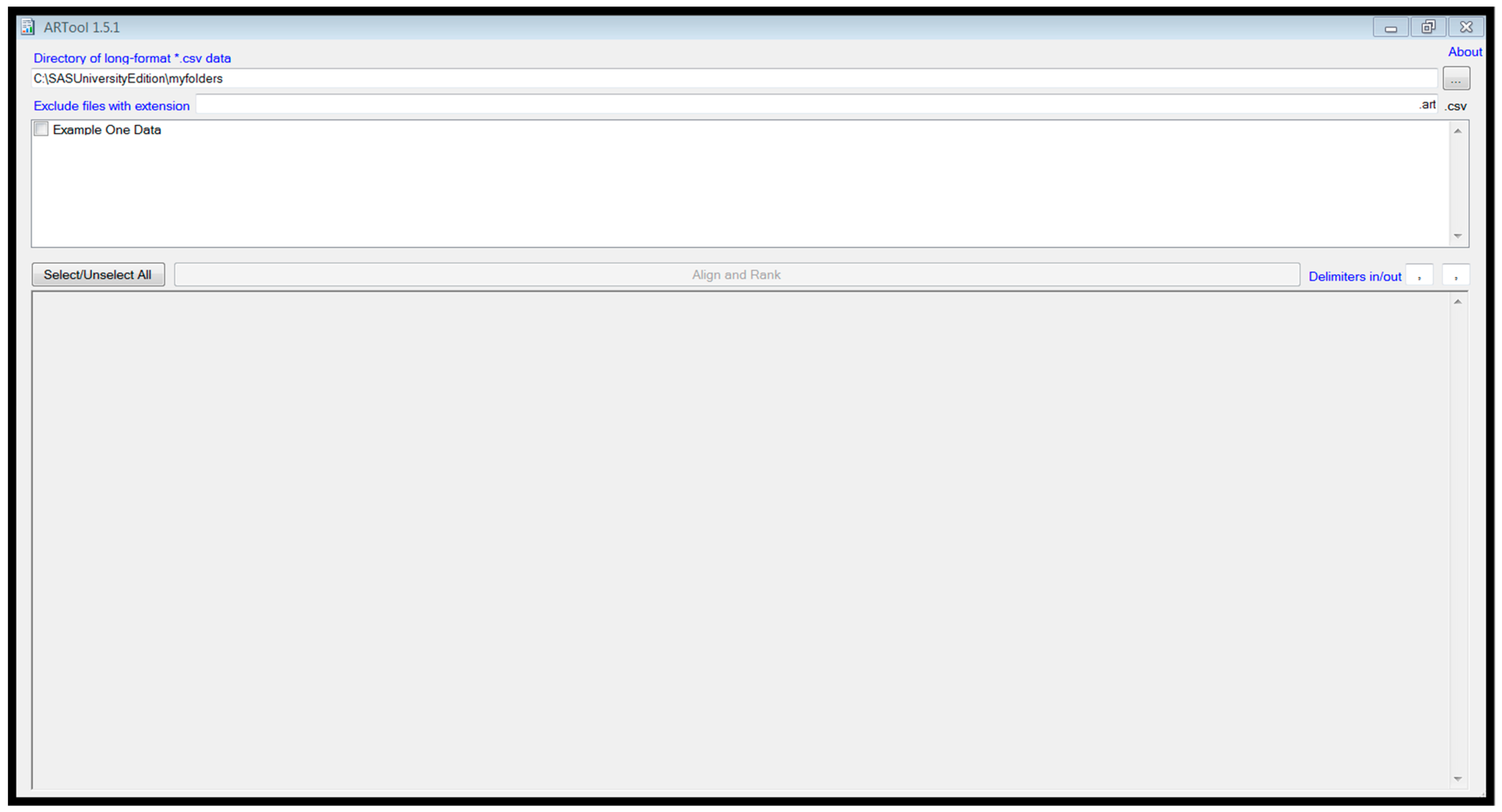
Start the ‘ARTool’ program. It should look like Figure 1 at startup.

The csv files in my ‘myfolders’ folder appear in the top window of the program. To process the data in the file and create an output data file, click the check-box next to the filename of the file for processing (Example One Data’) and click the ‘Align and Rank’ button in the lower right of the same window. A message will appear in the bottom window indicating that the file has been processed and that the output file has been created.

If there are problems, an error message will occur. The two most common errors are (1) the csv file is still being used by Excel and (2) blank spaces or non-numeric ‘Y’ values have been detected. For problem 1, close the csv file in Excel. Problem 2 may be a bit more complicated. First, check to make sure there are no observations with missing values indicated by blank spaces or a placeholder such as ‘.’. If this is the case, delete all rows in the original csv file where this occurs. Sometimes, the csv file has blank columns to the right of the ‘Y’ column or blank rows past the final observation of the csv file, either of which the ARTool program detects as a blank space and produce an error. To fix this, simply delete all the columns to the right of ‘Y’ and all the rows past the final observation, then resave the csv file.

With successful processing, a csv file will be generated by ARTool. Note that the file contains variable names in the first row which will include the ones we supplied in our CSV data file, as well as variables created by ARTool. For our example the variables were Rep, Nitrogen, Cultivar, Yield, aligned (Yield) for Nitrogen, aligned (Yield) for Cultivar, aligned (Yield) for Nitrogen*Cultivar, ART (Yield) for Nitrogen, ART (Yield) for Cultivar and ART (Yield) for Nitrogen*Cultivar. Also note that in the case of the completely random design, Rep is the same as OBS (Rep does not enter statistical modelling of a completely random design as a source of variation).

The ARTool generated csv file is used directly in the second SAS program for an analysis of variance (ANOVA), testing for nitrogen and cultivar main effects and an interaction between the two. Using the first row of the ‘data.art.csv’ file in our input statement and indicating the new file name in the ‘infile’ statement, we generated the following SAS program and results. Please note that the variable names were modified to facilitate easier SAS programing. Also note that the ‘aligned’ variables were not used in the analysis so they were labeled ‘a, b and c’. The analysis variables were the ART (aligned and rank transformed) variables generated by the ARTool program. Their names were shortened as well to ‘Anit, Acult and Anitcult’, and are used in the ANOVA.

The ART value for each factor or the interaction is the Y value stripped of all effects except the one under consideration during the aligning and ranking procedure. For example, Anit is the value of Y (yield) stripped of all cultivar and nitrogen–cultivar effects, Acult is Y (yield) stripped of all nitrogen and nitrogen–cultivar effects, and Anitcult is Y (yield) stripped of all nitrogen and cultivar main effects. The significance value for each tested source of variation was obtained from the test for the effect indicated in the Anit, Acult or Anitcult variable name. Thus, to obtain a significance value for nitrogen, examine the significance of the nitrogen effect on the Anit variable. For a cultivar effect, examine the significance of cultivar with Acult and for the interaction, nitrogen–cultivar, examine the nitrogen–cultivar effect with Anitcult.

The SAS program for performing a full factorial analysis of the data is presented below.

Title ‘Example One Program 2’;

data one;

infile ‘/folders/myfolders/Example One Program 1 Data.art.csv’ dlm = ‘,’ firstobs = 2;

input rep nit $ cult $ yield a b c Anit Acult Anitcult;

cards;

run;

proc anova;

classes nit cult;

model yield Anit Acult Anitcult = nit cult nit*cult;

means nit cult/lsd lines;

means nit*cult;

run;

Note that the model statement has as dependent variables yield (non-transformed yield values), Anit (ART values for Y considering only nitrogen), Acult (ART values for Y considering only cultivar, and Anitcult (ART values for Y considering only nitrogen–cultivar). The results of the analysis are discussed below.

In the ANOVA of non-transformed data, the p-values for nitrogen, cultivar and nitrogen–cultivar were 0.8345, 0.9002 and 0.2654, respectively. However, these values are not valid since the data did fulfilled the assumptions of normality. To consider the nitrogen effect for transformed data, consider the significance of the nitrogen effect for the dependent variable Anit. The p-value for nitrogen is 0.8322, which is not much different than the p-value produced for non-transformed data (0.8345). The difference is the level of confidence one can have in asserting that there is not a significant effect of nitrogen on yield when considering results from the transformed analysis. One cannot be confident in asserting this using the analysis of non-transformed data since the data were identified as non-normal in the initial test for normality performed in Program 1. Similarly, the same is true for cultivar and the nitrogen–cultivar interaction. Note that with all three analyses of transformed data, the p-value for the effects not being considered in each analysis (i.e., for cultivar and nitrogen–cultivar in the analysis for a nitrogen main effect) is close to 1.00. This is a characteristic of the analysis that provides somewhat of a verification of the effectiveness of the ART procedure. If these p-values are far from 1.00, the ART procedure may not be adapted to your data [1] and another method should be employed. Alternatives to the ART procedure were provided by Sawilowsky [10] and Higgins [11]. Fortunately, most data are amenable to the ART procedure.

3.2. Example Two—Randomized Complete Block Design

If the treatments from example one were set out in a randomized complete block design (RCBD), the ART process would be exactly like the one used in example one. The difference in the analyses of the two experimental designs is in the SAS model statement. With the RCBD, an effect attributable to blocking would be accounted for in the model statement and the analysis would resemble that shown below.

Title ‘Example Two’;

data one;

infile ‘/folders/myfolders/Example Two Data.art.csv’ dlm = ‘,’ firstobs = 2;

input rep nit $ cult $ yield a b c Anit Acult Anitcult;

cards;

run;

proc anova;

classes blk nit cult;

model yield Anit Acult Anitcult = blk nit cult nit*cult;

run;

The interpretation would be similar to example one and the p-values for non-transformed and transformed data are presented in

Table 1. p-values for ANOVA of non-transformed and transformed yield data of example 2.

	p-Value
Source of Variation	Non-Transformed Yield	ART Transformed Yield
Nitrogen	0.8240	0.8247
Cultivar	0.8907	0.8678
Nitrogen X cultivar	0.2299	0.3131

for reference. Remember that when interpreting the SAS output, p-values are only valid for testing a nitrogen effect using the dependent variable Anit, for a cultivar effect using Acult and an interaction using Anitcult. With all three analyses of transformed data, the p-values for the effects not considered in each analysis were close to 1.00, indicating that the ART procedure is appropriate for the data [1].

3.3. Example Three—Split Plot Design

This example is a little more complicated and considers an experiment where six rates of three nitrogen sources were evaluated for strawberry yield (g·plant⁻¹). The experimental design was a split plot with nitrogen source as the main plot and nitrogen rate as the sub-plot. There were five replicates of the main plot and the main plots were set in a randomized complete block design. Data are provided as the supplementary file ‘Example Three Data.csv’.

The SAS program for evaluating data normality and variance homogeneity is presented below.

Title ‘Example Three’;

data one;

infile ‘/folders/myfolders/Example Three Data.csv’ dlm = ‘,’ firstobs = 2;

input blk nit $ rate yield;

cards;

run;

proc print;

proc univariate normal;

var yield;

run;

proc anova;

classes nit rate;

model yield = nit;

means nit/HOVTEST = levene;

run;

proc anova;

classes nit rate;

model yield = rate;

means rate/HOVTEST = levene;

run;

proc anova;

classes nit rate;

model yield = nit*rate;

means nit*rate/HOVTEST = levene;

run;

proc anova;

classes blk nit rate;

model yield = blk nit blk*nit rate nit*rate;

test h = nit e = blk*nit;

run;

The Shapiro–Wilks normality test for this data produced a Shapiro–Wilk W statistic of 0.962988 with a Pr < W = 0.0116, indicating that the data is not normally distributed. The data does, however, seem to have homogeneous variances, as determined by Levene’s test. The ARTool app should thus be used to transform the data.

The analysis of the transformed data is straightforward.

title ‘Example Three’;

data one;

infile ‘/folders/myfolders/Example Three Data.art.csv’ dlm = ‘,’ firstobs = 2;

input blk nit $ rate yield a b c Anit Arate Anitrate;

cards;

run;

proc print;

run;

proc anova;

classes blk nit rate;

model yield Anit Arate Anitrate = blk nit blk*nit rate nit*rate;

test h = nit e = blk*nit;

run;

Note that for a split plot experiment, the correct test for the main plot must be explicitly requested (test h = nit e = blk*nit).

p-values are valid for testing a nitrogen effect using the dependent variable Anit, for a rate effect using Arate and an interaction using Anitrate. With all three analyses of transformed data, the p-values for the effects not considered in each analysis are close to 1.00, thus, the ART procedure is valid.

A comparison of p-values for analysis of non-transformed and transformed data is presented in

Table 2. p-values for ANOVA of non-transformed and transformed yield data of example 3.

	p-Value
Source of Variation	Non-Transformed Yield	ART Transformed Yield
Nitrogen	<0.0001	<0.0001
Rate	0.1617	0.0095
Nitrogen X rate	0.0795	0.0073

.

No data transformation an ANOVA reveals a significant effect of nitrogen source (p-value < 0.0001), and non-significant effects of the nitrogen rate (α = 0.1617) and the interaction between the two (p-value = 0.0795). Confidence in these assertions is not high, based on the fact that the data are not normally distributed, thus, the test power is not high and the chances of a type I error are relatively high. When the data are appropriately transformed, all three sources of variation are significant at (p-values = 0.0001, 0.0095 and 0.0073 for source, rate and interaction, respectively) and the confidence in these assertions is high, since the ANOVA is legitimate with transformed data.

The significant interaction suggests that the next appropriate step in the analysis would be to determine if there is a rate effect for each source of nitrogen separately.

To do this, the data must be separated into three files—one corresponding to each source of nitrogen. Each data set should be ART transformed separately if suggested by the test for normality. This would require separate csv files for each data set.

3.3.1. Urea

The SAS code for evaluating Urea is illustrated below.

title ‘Example Three Urea’;

data one;

infile ‘/folders/myfolders/Example Three Data Urea.art.csv’ dlm = ‘,’ firstobs = 2;

input blk rate yield a Arate;

cards;

run;

proc print;

proc univariate normal;

var yield;

run;

proc anova;

classes blk rate;

model yield Arate = blk rate;

run;

The results suggest that the data is not normally distributed therefore transformed data should be used for estimating significance of the rate effect. The rate effect for the source Urea has a p-value = 0.6779, thus the rate does not seem to impact the yield response when using Urea as a nitrogen source.

3.3.2. Calcium nitrate

The evaluation of the rate effect for calcium nitrate proceeds in a similar fashion using the following SAS code.

title ‘Example Three Calcium Nitrate’;

data one;

infile ‘/folders/myfolders/Example Three Data Calcium Nitrate.art.csv’ dlm = ‘,’ firstobs = 2;

input blk rate yield a Arate;

cards;

run;

proc print;

proc univariate normal;

var yield;

run;

proc anova;

classes blk rate;

model yield Arate = blk rate;

run;

Since the data appear to be normally distributed, non-transformed data can be used for the estimation of rate significance with calcium nitrate. There is a significant rate effect (p-value = 0.0100), thus, a linear regression to estimate the relationship between yield and rate would be appropriate as the next step in the analysis. The reader is left to pursue this on their own.

3.3.3. Potassium Nitrate

The evaluation of the rate effect for potassium nitrate (SAS code below) suggests that the data are not normally distributed, thus transformed data should be used for the estimation of rate significance with potassium nitrate. There is a significant rate effect (p-value = 0.0506), thus a linear regression to estimate the relationship between yield and rate would be appropriate as the next step in the analysis.

title ‘Example Three Potassium Nitrate’;

data one;

infile ‘/folders/myfolders/Example Three Data Potassium Nitrate.art.csv’ dlm = ‘,’ firstobs = 2;

input blk rate yield a Arate;

cards;

run;

proc print;

proc univariate normal;

var yield;

run;

proc anova;

classes blk rate;

model yield Arate = blk rate;

run;

The reader is left to evaluate the linear relationship between rate and yield for calcium nitrate on their own since data was normally distributed. Here, with potassium nitrate, data are not normally distributed and an illustration of the procedure with non-normal data is appropriate. The p-values for the significance levels of the regression relationship between the rate of potatssium nitrate and the yield should be estimated using transformed data. The parameter estimates are obtained using non-transformed data. The SAS code presented below illustrates this method.

title ‘Example Three Potassium Nitrate Regression’;

data one;

infile ‘/folders/myfolders/Example Three Data Potassium Nitrate.art.csv’ dlm = ‘,’ firstobs = 2;

input blk rate yield a Arate;

rate2 = rate*rate;

cards;

run;

proc reg;

model yield Arate = rate;

model yield Arate = rate rate2;

run;

The linear and quadratic nature of the relationship will be examined. Note that a variable ‘rate2′ was generated in line 5 of the SAS code. This enables testing for the quadratic effect. The model statements in lines 9 and 10 used in the regression procedure of SAS will test for a linear component followed by a quadratic component. The p-values were obtained from the tests on Arate, while the parameter estimates were extracted from the tests evaluating yield.

Neither linear nor quadratic components were significant, as revealed in the regression analysis. One might question why the rate was significant (p-value = 0.0506) but neither linear (p-value = 0.1839) nor quadratic (p-value = 0.0899) components are significant. This apparent contradiction suggests that while there is a relationship between rate and yield, this relationship is not linear. Further analysis could investigate non-linear models. Additionally, the rate effect was marginally significant and one might argue that a p-value of 0.0899 for a quadratic response is also marginally significant.

For illustrative purposes, suppose that the significance level of the quadratic component (p-value = 0.0899) is sufficient so that we need to derive the regression equation for a presentation. These estimates would be obtained from the analysis of non-transformed data. The regression equation would be:

$$Y=344.2+16.6\ast rate-3.2\ast {rate}^2$$

Since there seems to be a relationship between rate and yield using potassium nitrate, further experiments could investigate a broader range of rates with a greater number of replications to determine if the quadratic component in the initial experiment was indeed relevant. Non-linear models could also be examined.

3.4. Other Designs and Experiments

The beauty of the ART procedure is that it is applicable to nearly any situation and easy to use. The main consideration for use in any situation is to make sure to use the correct effect when performing significance tests, i.e., using the test for Atreatment when testing for the treatment effect, etc.

4. Conclusions

Researchers often use statistical techniques because they are familiar with them, even though they may not be appropriate or valid if data are not normal or if they have heterogenous variances. Many of the most commonly used statistical techniques in horticultural research are parametric techniques, which are valid only if they are used on normal data. When these procedures are used on non-normal data, power (the probability of detecting a treatment effect when it does in fact exist) is reduced and the probability of a type I error (declaring a significant treatment effect exists when it in fact does not) increases. The ART procedure is a valuable method for non-parametric testing of both main effects and interactions using standard ANOVA techniques. This study provided step-by-step instructions for downloading and installing SAS and the ART app, as well as step-by-step illustrations of the use of the ARTool program with SAS for data analysis to encourage readers to adopt this methodology in their own work when appropriate.