A Stability and Accuracy Evaluation of CNN, LR and GA-BP Models for Pepper Leaf Disease Recognition Based on a Multi-Dimensional Visual Feature Dataset

Highlights

What are the main findings?

• Lab b-channel segmentation performs best for pepper leaf preprocessing; 25 discriminative fused visual features are retained after random-forest screening.
• Twenty repeated tests prove CNN has top accuracy and stability, followed by LR, while GA-BP shows poor prediction performance.

What are the implications of the main findings?

• The standardized preprocessing and feature screening scheme offers unified references for crop leaf disease identification research.
• The model comparison results guide targeted algorithm deployment for high-precision diagnosis and low-consumption embedded field devices.

Abstract

Pepper suffers from bacterial leaf spot and yellow leaf curl, which substantially reduce crop yield and fruit quality. Traditional manual diagnosis suffers from delayed response, subjective bias and heavy labor consumption, while existing intelligent detection pipelines lack standardized preprocessing workflows, quantitative feature screening and systematic model comparison. To fill these research gaps, we built a pepper leaf dataset with 1260 samples (healthy, bacterial spot, yellow leaf curl). Three segmentation algorithms (Lab b-channel, RGB super-green, Otsu-ACWE) were quantitatively assessed to select the optimal preprocessing scheme. We extracted 32 fused visual features (27 RGB/HSV/Lab color moments + five gray-level co-occurrence matrix (GLCM) texture metrics) and adopted a random-forest classifier to eliminate seven low-contribution redundant features, retaining 25 discriminative variables. Three representative models, namely convolutional neural network (CNN), logistic regression (LR), and genetic-algorithm-optimized back-propagation neural network (GA-BP), were constructed for parallel comparison via 20 independent repeated trials, with accuracy, precision, recall, F1-score and area under the receiver operating characteristic curve (AUC) as evaluation indicators. The results verified that Lab b-channel segmentation achieved superior background separation and intact lesion edge retention. CNN yielded the best performance, with an average test accuracy of 97.67% and an average AUC of 0.999, accompanied by minimal metric standard deviations and outstanding stability. LR exhibits low computational cost and fast training, which is promising for applications with limited computing resources. In contrast, GA-BP shows weak nonlinear fitting ability and severe prediction fluctuations, making it unsuitable for high-precision diagnosis. This study proposes a standardized experimental framework to offer theoretical guidance and algorithmic references for intelligent vegetable leaf disease identification. All experiments were conducted on a dataset collected under standardized indoor single-illumination conditions; therefore, the conclusions of this study are only applicable to such controlled scenarios.

1. Introduction

Pepper is an economically valuable vegetable crop widely cultivated worldwide, possessing dual edible and processing values. The planting scale and yield of pepper directly determine the economic profits of the vegetable industry and the stable income of growers. During the growth period, pepper plants are susceptible to leaf diseases caused by microbial infection, among which bacterial leaf spot and yellow leaf curl are two prevalent typical diseases in fields [1,2]. After plants are infected by pathogens, leaf tissues show chlorosis and necrosis, and the photosynthetic efficiency of leaves decreases significantly. These two widespread pepper diseases can cause substantial field-scale yield losses, and severe pathogen infection may lead to whole-plant wilting and complete crop failure [2,3]. Traditional disease diagnosis depends on manual field observation by plant-protection technicians, a method that suffers from delayed response, severe subjective discrimination errors, and high labor consumption under large-scale cultivation conditions [4]. In addition, disease symptoms are inconspicuous in the early onset stage, making it difficult for manual observation to accurately distinguish healthy leaves from mildly diseased leaves. This easily misses the optimal prevention and control window, resulting in excessive pesticide application and degraded agricultural product quality [5].

With the in-depth application of computer vision and machine-learning technologies in precision agriculture, numerous studies have demonstrated that leaf-image-based automatic crop disease identification serves as an important technical approach for plant-protection monitoring. Existing research on crop disease identification is divided into two major technical systems: the first is an end-to-end recognition scheme based on deep convolutional neural networks, which automatically extracts deep semantic information from images without manual feature design; the second extracts shallow visual features such as color and texture manually and combines them with traditional machine-learning classifiers for disease discrimination, featuring interpretable features, low computing power requirements, and easy deployment on miniature devices [6,7,8]. Although the two schemes have respective advantages and disadvantages, current research on pepper leaf disease detection still has obvious shortcomings:

• The existing preprocessing schemes lack standardized technical specifications. Leaf images captured under field conditions contain complex background interference including soil, weeds and plastic mulch; directly feeding unprocessed images into classification models will introduce massive noise and degrade model performance. Most existing studies adopt a single background segmentation algorithm without quantitative comparison of multiple segmentation methods, making it hard to screen the optimal preprocessing strategy suitable for pepper leaves [9,10].
• Lack of quantitative basis for feature screening. Most studies only extract single RGB color features without fusing multi-space color features (HSV, Lab) and gray-level co-occurrence matrix (GLCM) texture features. Moreover, low-contribution redundant features are not eliminated through quantitative feature importance evaluation. Redundant feature dimensions increase computational consumption and reduce classification stability [11,12].
• Single dimension of model comparison. Most existing studies on pepper disease recognition only compare one or two algorithms, lacking parallel comparison of three representative models including convolutional neural networks, linear machine learning, and intelligent optimized neural networks. Few studies conduct repeated experiments multiple times to eliminate random errors, leading to the low credibility of evaluation results for model generalization performance and stability [13,14].

To solve the above problems, this study takes healthy pepper leaves, leaves infected with bacterial leaf spot, and leaves with yellow leaf curl as research objects, and constructs a pepper leaf disease image dataset containing 1260 samples. First, three background segmentation algorithms including Lab-b channel segmentation, RGB super-green feature segmentation, and Otsu-ACWE are compared to achieve accurate segmentation of leaf images. Second, color moment features from three color spaces (RGB, HSV, Lab) and GLCM texture features are fused, and random forest is used to sort feature importance, removing low-contribution features to obtain 25-dimensional effective discriminative features. Finally, three recognition models, namely convolutional neural network (CNN), logistic regression (LR), and genetic-algorithm-optimized BP neural network (GA-BP), are built. Multiple evaluation metrics including accuracy, precision, recall, F1-score, AUC, and standard deviation of indicators are adopted, and 20 repeated experiments are carried out to quantitatively compare the recognition accuracy and operational stability of the three models, so as to screen the optimal algorithm for pepper leaf disease recognition. Given that the dataset in this work was acquired under standardized indoor conditions, this research can provide standardized references for image preprocessing, multi-dimensional visual feature extraction, and multi-model comparative experimental design of vegetable leaf diseases. Meanwhile, it offers theoretical support and an algorithm basis for developing intelligent disease-recognition approaches for pepper. Model evaluation in this study was performed strictly on the independent test set rather than training or validation subsets to guarantee reliable generalization assessment.

2. Materials and Methods

2.1. Materials

The pepper leaf disease dataset used in this study was obtained from publicly shared online resources. The pepper species involved in the dataset was chili (Capsicum annuum). Since these images are secondary shared materials collected from the internet, some original metadata including acquisition start–end date, shooting time period, planting environment (field/greenhouse), camera or mobile phone model, and original image resolution cannot be traced. A total of 1260 leaf samples were screened and sorted in this study, consisting of 420 healthy leaf samples, 420 samples infected with bacterial leaf spot, and 420 samples suffering from yellow leaf curl disease. All disease leaf samples were originally naturally infected under field conditions. The stratified sampling strategy was adopted to divide the whole dataset into a training set, a validation set and a test set with a fixed 4:1:1 ratio (66.7%/16.7%/16.7%), which ensures consistent class distribution among the three subsets. Specifically, 840 samples were assigned to the training set, 210 samples to the validation set, and the remaining 210 samples served as the independent test set for unbiased model evaluation.

2.2. Methods

2.2.1. Image Data Processing Methods

Irrelevant objects in the image background were removed to retain only the leaf region and contour. The background usually contains redundant information unrelated to the target, which interferes with feature extraction and leads to inaccurate feature values. In severe cases, it may hinder model convergence or induce overfitting [15]. In this study, three background segmentation methods were adopted and compared to select an optimal background segmentation strategy. All segmentation experiments were conducted with a fixed random seed to reduce randomness. Segmentation performance was quantitatively evaluated using Intersection over Union (IoU) and Dice coefficient; manual pixel-wise annotations served as the ground-truth reference for calculating these metrics.

(1)

Background segmentation method based on the Lab b-channel

This algorithm integrates color-space transformation and global-threshold segmentation derived from b-channel statistics. First, the original RGB image is converted into the Lab color space to amplify the chromatic difference between leaf tissues and complex backgrounds using the b-channel component. Afterwards, threshold segmentation and morphological postprocessing are implemented to complete background elimination [16]. The segmentation threshold T was calculated as the sum of the b-channel mean value (μ_b) and 0.2 times the b-channel standard deviation (σ_b). Here, μ_b represents the mean intensity of the b-channel, and σ_b represents its standard deviation. Morphological operation parameters: opening operation with disk-shaped structural element (radius = 1 pixel); closing operation with disk-shaped structural element (radius = 20 pixels); small noise regions were removed by area filtering with the minimum reserved area set to 500 pixels.

(2)

Background segmentation method based on RGB super-green features

Different from the above method, this approach enhances the distinction between leaves and background by extracting RGB super-green features for background segmentation [17]. This algorithm was only included for comparative analysis and was not applied in the practical processing pipeline of this study.

(3)

Background segmentation method based on Otsu-ACWE

This algorithm integrates the Otsu threshold-segmentation and Chan-Vese Active Contour Without Edges (ACWE) model. After calculating the chromaticity modulus in the Lab color space, the Otsu automatic threshold is used to generate a rough leaf mask. Taking this coarse mask as the initialization condition, the Chan-Vese active contour is iteratively executed on the gray-scale image to refine leaf boundaries, and finally a white-background matting result is obtained [18,19]. The iteration number, smoothing coefficient and weighting parameters for the ACWE model were not calibrated in this work; this approach was only used for comparison and was not adopted for the subsequent image processing workflow.

All image segmentation, visual feature extraction and model-building procedures were implemented using MATLAB R2023b (MathWorks, Natick, MA, USA). The image processing workflow was developed based on the Image Processing Toolbox; the random forest, logistic regression, GA-BP neural network and statistical analysis modules relied on the Statistics and Machine Learning Toolbox; the convolutional neural network was built with the Deep Learning Toolbox embedded in MATLAB R2023b.

2.2.2. Feature Extraction Methods

In this research, both color and texture features were extracted from leaf images for subsequent disease identification.

(1)

Color features

Color features are among the most widely used visual descriptors in image processing and computer-vision research, and can be derived from multiple color spaces including RGB, HSV, Lab, YCrCb, and YUV. To capture color phenotypic differences caused by leaf lesions, features were extracted from the RGB, HSV, and Lab color spaces in the present work.

The RGB color space comprises three channels, red, green, and blue, and is the most commonly used color space. The HSV color space is designed according to human visual perception and describes colors via three mutually independent dimensions: Hue, Saturation, and Value. Compared with RGB, HSV better matches human intuitive color perception. Lab is a standard color system defined by the International Commission on Illumination (CIE) and offers the key advantage of perceptual uniformity, which is suitable for describing subtle color changes in diseased plant tissues. For each channel within the three selected color spaces, the first-order moment (mean), second-order moment (standard deviation), and third-order moment (skewness) were computed. Nine color features were obtained for each color space, producing 27 color features in total [20,21,22,23].

(2)

Texture features

Popular texture-extraction algorithms include the gray-level co-occurrence matrix (GLCM), Gray-Level Run Length Matrix (GLRM), and Local Binary Pattern (LBP). Considering the fine gray-scale heterogeneity of lesion regions, GLCM was selected in this study to extract the texture features of diseased pepper leaves. Essentially, GLCM characterizes the joint probability distribution of pixel pairs and has symmetric properties. It can comprehensively reflect the variation degree of image gray levels in different directions and intervals, as well as the position distribution of pixels with identical gray values, which serves as a critical basis for calculating image texture features. The GLCM was calculated with an offset distance of 1 pixel in four directions (0°, 45°, 90°, 135°); the final texture metrics were averaged across the four directions to eliminate directional bias. Five texture metrics were calculated, including entropy (ENT), angular second moment (ASM), correlation (COR), inverse difference moment (IDM), and contrast (CON) [24,25,26].

Entropy (ENT): This metric quantifies the randomness of image texture. Entropy reaches its maximum value when all GLCM elements are identical and declines if element values are highly uneven. A higher entropy value corresponds to a more randomly distributed gray-scale, as formulated in Equation (1):

$$ENT=-{\displaystyle \sum _{i=1}^k}{\displaystyle \sum _{j=1}^k}G(i,j){log}_{2}G(i,j)$$

(1)

Angular second moment (ASM): It is the sum of squares of all elements in GLCM, representing the uniformity of gray distribution and texture coarseness. ASM takes a large value when element values are uniform and a small value when element values differ greatly, as shown in Equation (2):

$$ASM={\displaystyle \sum _{i=1}^k}{\displaystyle \sum _{j=1}^k}G{(i,j)}^2$$

(2)

Correlation (COR): It measures the similarity of elements in rows or columns of GLCM and reflects the local gray correlation of images. The correlation value is large when matrix elements are uniform and equal, and small when elements differ drastically; textures with directional consistency correspond to high correlation values, as expressed in Equation (3):

$$COR={\displaystyle \frac{{\displaystyle {\sum }_{i=1}^k}{\displaystyle {\sum }_{j=1}^k}(i-{\mu }_x)(j-{\mu }_y)G(i,j)}{{\sigma }_x{\sigma }_y}}$$

(3)

Inverse difference moment (IDM): It quantifies local variations in image texture. A high IDM value indicates minor local changes and uniform texture regions, as formulated in Equation (4):

$$IDM={\displaystyle \sum _{i=1}^k}{\displaystyle \sum _{j=1}^k}{\displaystyle \frac{G(i,j)}{1+{(i-j)}^2}}$$

(4)

Contrast (CON): It refers to the inertia moment near the main diagonal, measuring the distribution of matrix values and local gray changes, and representing image clarity and texture depth. Deeper texture grooves correspond to higher contrast and clearer images, as defined in Equation (5):

$$CON={\displaystyle \sum _{i=1}^k}{\displaystyle \sum _{j=1}^k}{(i-j)}^{2}G(i,j)$$

(5)

2.2.3. Sample Partitioning Method

To avoid category imbalance and ensure consistent sample distribution across subsets, stratified random sampling at the leaf level was adopted to maintain stable class proportions during dataset partitioning. A fixed random seed was utilized throughout the partitioning process to ensure experimental repeatability and result reproducibility. All leaf samples were randomly divided into training, validation, and test subsets at a fixed 4:1:1 ratio. Specifically, 840 samples were assigned to the training set, 210 samples to the validation set, and the remaining 210 samples to the independent test set for unbiased model evaluation.

2.2.4. Model Construction Method

In this study, convolutional neural network (CNN), logistic regression (LR), and genetic-algorithm-optimized back-propagation neural network (GA-BP) were selected for comparative modeling for the following reasons: CNN is a typical end-to-end deep-learning framework capable of automatically extracting high-level semantic features from raw leaf images; LR is a classic linear machine-learning algorithm with low computational overhead; GA-BP combines the global-optimization capability of genetic algorithms with a BP neural network to address nonlinear regression-classification problems and has been widely applied in agricultural disease-recognition tasks. A random-forest classifier was employed to rank feature importance and screen out redundant and low-contribution features. All model experiments were executed with a fixed random seed, and 20 independent replicate runs were implemented to reduce random experimental errors. Dataset partitioning was performed at the leaf level, where each complete leaf image was treated as one individual sample [27,28,29].

Model hyper-parameter settings:

(1)

CNN

Input image size: 224 × 224; input channel: 3 (RGB); resize interpolation mode: bilinear; loss function: cross-entropy loss; epoch = 800; learning rate = 0.001; optimizer: sgdm; regularization strategy: dropout; network layer number and filter size: three-layer convolutional network, convolution kernel size [3 × 3, 3 × 3, 3 × 3], followed by max-pooling layers and fully connected layers.

(2)

LR

Input features: the pre-screened 25-dimensional visual discriminative features; class-balance strategy: none (original sample class proportions were retained); solver: lbfgs; regularization penalty: ridge regression with λ = 0.00023.

(3)

GA-BP

Input features: the pre-screened 25-dimensional visual discriminative features; GA optimization object: weights and biases of the BP neural network; population size = 20; evolution generation = 40; crossover probability = 0.7; mutation probability = 0.01; class-balance strategy: none (original sample class proportions were retained).

(4)

Random forest

Number of decision trees (n_estimators) = 100; split criterion: curvature; maximum tree depth = unlimited; sample weight setting: default equal-weighted samples; other key hyper-parameters: minimum leaf size = 10, number of predictors to sample = 6, random seed rng = 42, out-of-bag (OOB) prediction and feature importance calculation were activated.

All model-building procedures adopted the same MATLAB R2023b environment and toolboxes described in Section 2.2.1.

2.2.5. Model Evaluation Method

This study implemented a three-category classification task to discriminate healthy pepper leaves, leaves infected with bacterial leaf spot, and leaves infected with yellow leaf curl disease. For models that output class probabilities via the softmax activation function, the final predicted label was assigned to the category with the highest predicted probability. To detect statistically significant performance differences across competing models, evaluation metrics collected from 20 independent replicate experiments were used for statistical analysis. Specifically, the Shapiro–Wilk test was applied to examine the normality of metric distributions, and the Levene test was employed to check the homogeneity of variance. One-way analysis of variance (ANOVA) combined with post hoc multiple comparison tests was subsequently conducted to identify pairwise significant differences between different models.

The confusion matrix and derived indicators including accuracy, precision, recall and F1-score were used to quantify the performance of disease detection algorithms, with corresponding calculation formulas shown in Equations (6)–(9). For this three-category classification task, precision, recall and F1-score were calculated using macro-average to obtain unbiased overall performance metrics across all three leaf categories.

$$Accuracy={\displaystyle \frac{TP+TN}{TP+TN+FP+FN}}$$

(6)

$$Precision={\displaystyle \frac{TP}{TP+FP}}$$

(7)

$$Recall={\displaystyle \frac{TP}{TP+FN}}$$

(8)

$$F1-score={\displaystyle \frac{2\times Precision\times Recall}{Precision+Recall}}$$

(9)

3. Results

3.1. Preprocessing Outcomes of Pepper Leaf Images

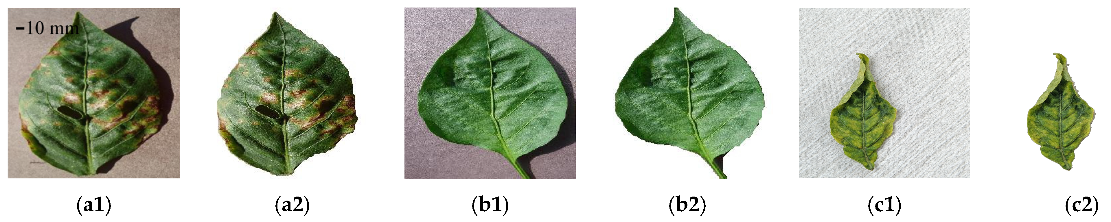
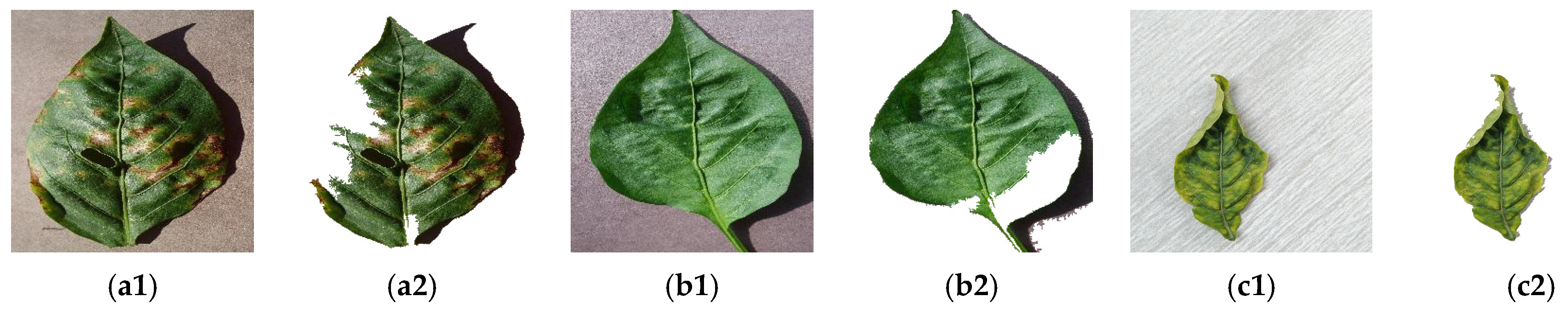
To eliminate complex background interference and preserve valid lesion features for subsequent modeling, three background segmentation algorithms, including the Lab-b channel segmentation, RGB super-green feature segmentation, and Otsu-ACWE segmentation, were implemented to preprocess raw leaf images, with visualized comparisons illustrated in Figure 1, Figure 2 and Figure 3. Both qualitative visual observation and quantitative evaluation based on Intersection over Union (IoU) and Dice coefficient were performed to comprehensively assess segmentation performance. All three algorithms successfully separated leaf foregrounds from complex field backgrounds filled with soil and weeds. Qualitative visual comparison indicated that the Lab-b channel segmentation accurately retained complete leaf contours and subtle lesion boundary details; the RGB super-green segmentation easily caused partial pixel loss and incomplete edge segmentation at leaf margins; and the Otsu-ACWE segmentation produced over-smoothed and slightly distorted leaf edges after iterative contour optimization, resulting in the loss of fine texture information. Comprehensive visual evaluation confirmed that the Lab b-channel method achieved the best performance in background removal integrity and diseased-region detail preservation, making it the optimal preprocessing strategy for pepper leaf disease images.

3.2. Extraction Results of Visual Features

3.2.1. Statistical Distributions of Lab Color Features

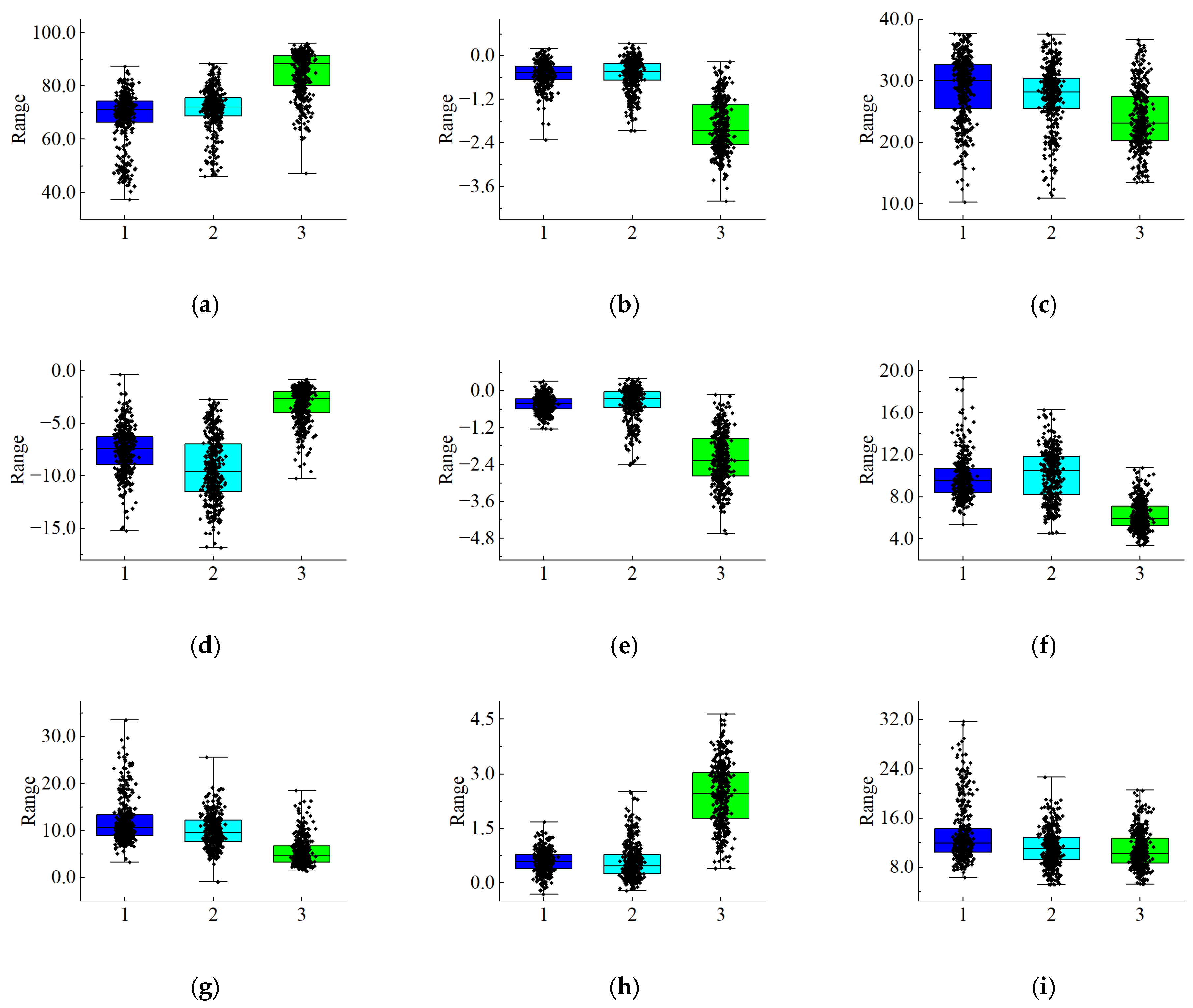
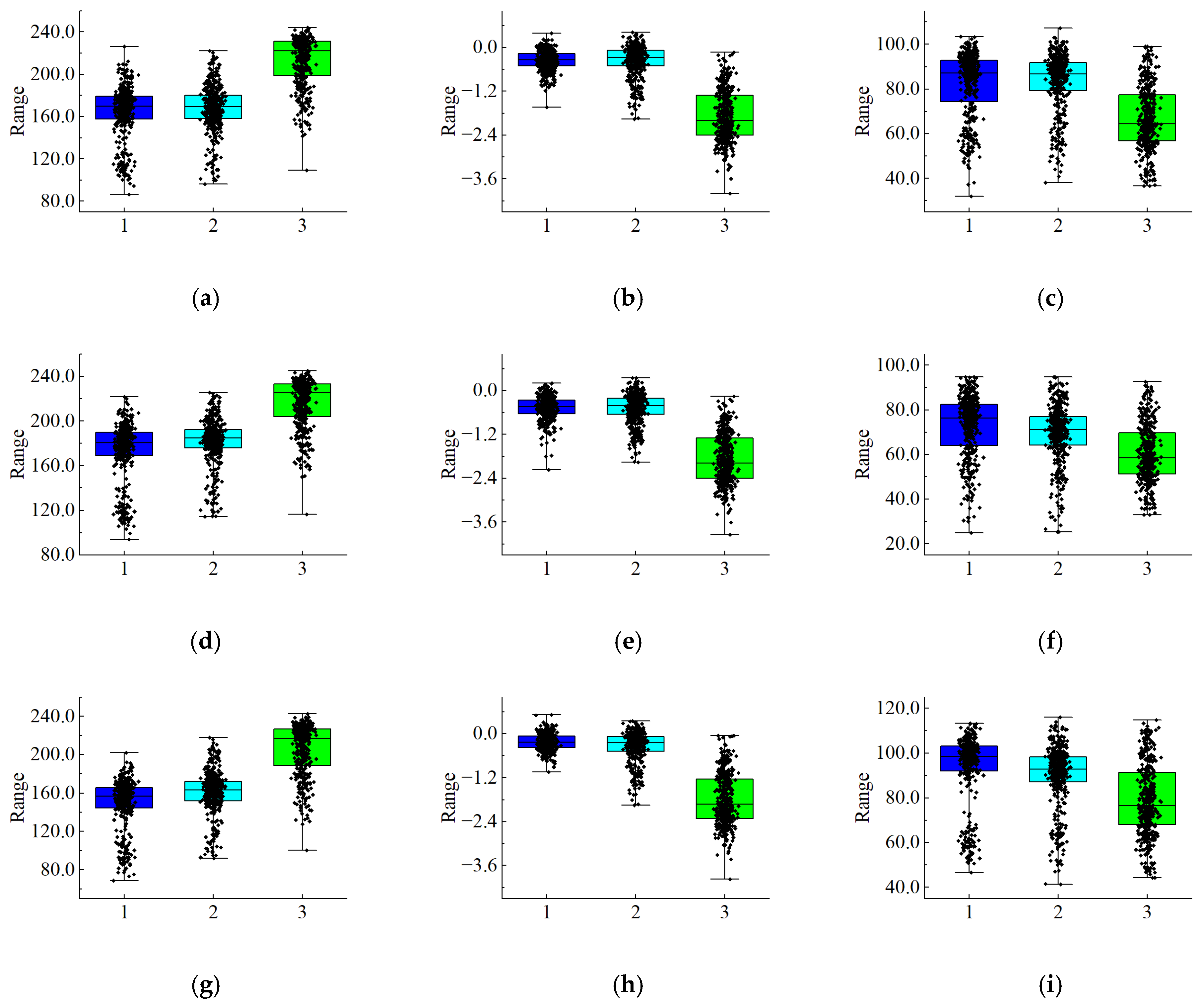
Nine statistical color metrics were calculated from the Lab color space, including the first-order moment (mean value), second-order moment (standard deviation), and third-order moment (skewness) for the L, a and b channels. Box-and-whisker plots showing the sample distribution of each feature are displayed in Figure 4, and the corresponding descriptive statistical values are summarized in

Table 1. Statistical results of Lab color features.

Feature	Bacterial Leaf Spot		Healthy Leaf		Yellow Leaf Curl
	Range	Mean	Range	Mean	Range	Mean
First moment (L)	0.09~0.63	0.20	0.04~0.58	0.20	0.01~0.38	0.08
First moment (a)	0.13~0.54	0.26	0.08~0.38	0.22	0.03~0.36	0.12
First moment (b)	0.38~0.89	0.69	0.47~0.88	0.72	0.46~0.96	0.85
Second moment (L)	0.11~0.39	0.19	0.04~0.38	0.17	0.04~0.16	0.09
Second moment (a)	0.15~0.43	0.28	0.15~0.41	0.25	0.12~0.39	0.25
Second moment (b)	0.10~0.37	0.29	0.11~0.37	0.27	0.13~0.36	0.24
Third moment (L)	−0.20~3.44	1.36	−0.49~2.50	0.91	−0.13~5.08	1.98
Third moment (a)	−0.20~1.85	0.82	−0.05~2.84	0.93	0.20~4.54	2.27
Third moment (b)	−2.04~0.22	−0.47	−1.96~0.34	−0.48	−3.96~−0.16	−1.88

. Obvious numerical stratification among the three leaf categories can be observed for the first-order moment of the L channel, the first-order moment of the b channel, and the third-order moment of the b channel. By contrast, the value ranges of the second-order moment of the a channel overlap considerably across the three groups, with inter-group differences smaller than 1.0. In addition, yellow leaf curl samples generally yield lower values for the second-order moment of the L channel and the third-order moment of the a channel compared with the other two categories.

3.2.2. Statistical Distributions of HSV Color Features

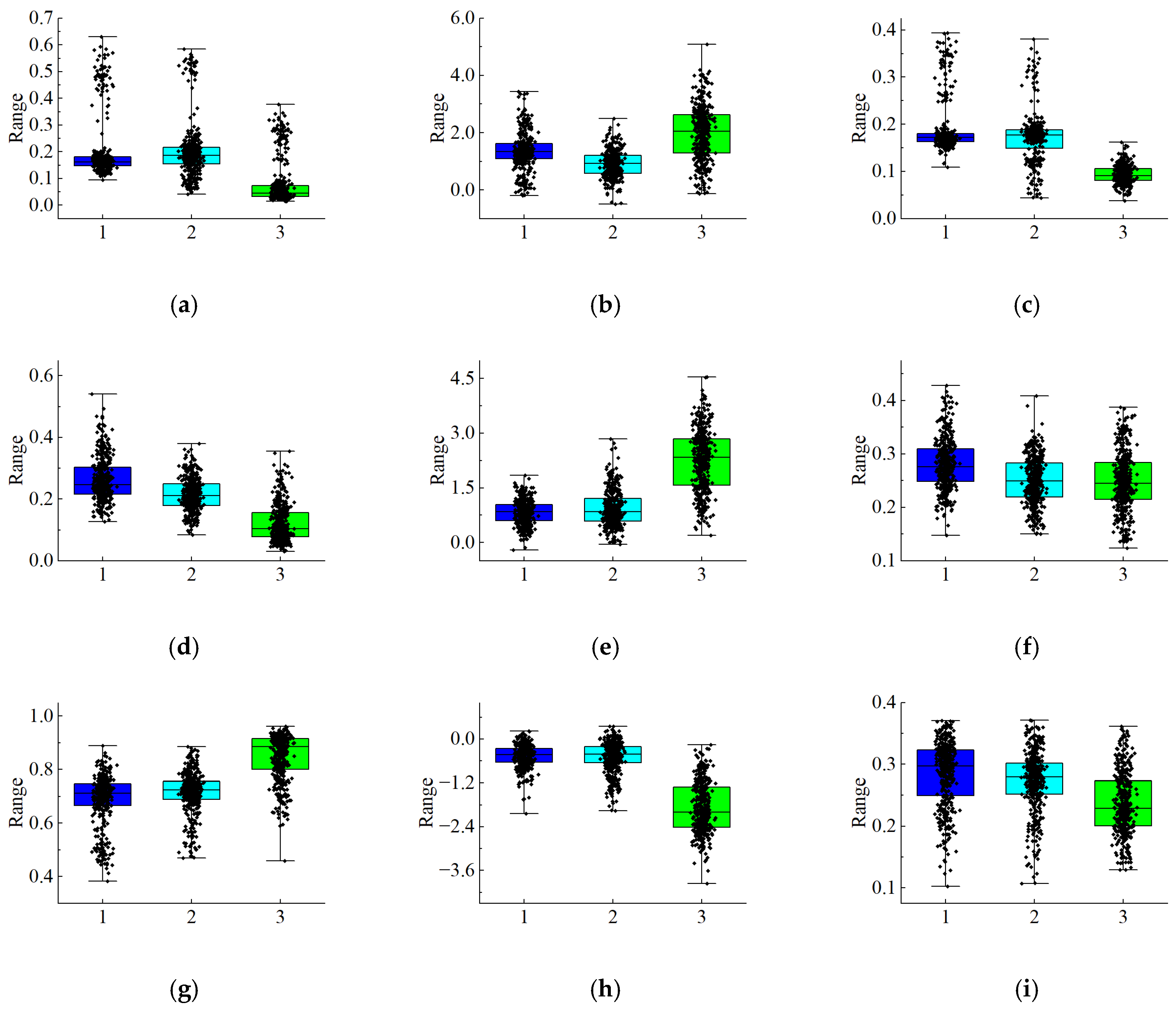
Nine descriptive color metrics were derived from the HSV color space, namely the first-order moment (mean), second-order moment (standard deviation), and third-order moment (skewness) corresponding to the H, S and V channels. The sample distribution of each feature is visualized in Figure 5, while the detailed descriptive statistics are summarized in

Table 2. Statistical results of HSV color features.

Feature	Bacterial Leaf Spot		Healthy Leaf		Yellow Leaf Curl
	Range	Mean	Range	Mean	Range	Mean
First moment (H)	0.09~0.63	0.20	0.04~0.58	0.20	0.01~0.38	0.08
First moment (S)	0.13~0.54	0.26	0.08~0.38	0.22	0.03~0.36	0.12
First moment (V)	0.38~0.89	0.69	0.47~0.88	0.72	0.46~0.96	0.85
Second moment (H)	0.11~0.39	0.19	0.04~0.38	0.17	0.04~0.16	0.09
Second moment (S)	0.15~0.43	0.28	0.15~0.41	0.25	0.12~0.39	0.25
Second moment (V)	0.10~0.37	0.29	0.11~0.37	0.27	0.13~0.36	0.24
Third moment (H)	−0.20~3.44	1.36	−0.49~2.50	0.91	−0.13~5.08	1.98
Third moment (S)	−0.20~1.85	0.82	−0.05~2.84	0.93	0.20~4.54	2.27
Third moment (V)	−2.04~0.22	−0.47	−1.96~0.34	−0.48	−3.96~−0.16	−1.88

. It should be noted that several HSV-derived features exhibited numerical ranges comparable to those obtained from the Lab color space, which is an inherent statistical property of the present pepper leaf dataset. The third-order moment of the S channel and the first-order moment of the V channel exhibit considerable value overlap across the three leaf groups, with inter-group differences in mean values all lower than 0.15. For yellow leaf curl samples, the overall values of the third-order moment of the H channel and the third-order moment of the S channel are notably higher than those of bacterial leaf spot and healthy leaf samples.

3.2.3. Statistical Distributions of RGB Color Features

Nine color-statistic descriptors were extracted from the RGB color space, including the first-order moment (mean), second-order moment (standard deviation), and third-order moment (skewness) for the R, G and B channels. The sample distribution of each feature is visualized in Figure 6, and the corresponding descriptive statistical results are listed in

Table 3. Statistical results of RGB color features.

Feature	Bacterial Leaf Spot		Healthy Leaf		Yellow Leaf Curl
	Range	Mean	Range	Mean	Range	Mean
First moment (R)	86.52~226.26	164.24	96.18~222.10	167.83	109.12~244.22	212.60
First moment (G)	93.96~221.49	173.43	114.14~225.46	182.19	116.47~245.08	216.19
First moment (B)	68.94~201.92	149.25	91.84~217.96	161.17	100.27~242.47	205.36
Second moment (R)	32.01~103.56	82.06	38.12~107.35	83.18	36.61~99.11	66.69
Second moment (G)	25.02~94.83	72.82	25.34~94.80	69.32	32.95~95.29	60.54
Second moment (B)	46.59~113.25	93.01	41.42~116.13	89.89	44.32~114.70	79.11
Third moment (R)	−1.63~0.38	−0.36	−1.96~0.41	−0.37	−3.39~−0.14	−1.87
Third moment (G)	−2.17~0.21	−0.47	−1.96~0.35	−0.49	−3.95~−0.16	−1.87
Third moment (B)	−1.04~0.52	−0.23	−1.94~0.34	−0.35	−3.97~−0.05	−1.78

. The second-order moment of the R channel, the second-order moment of the G channel, and the third-order moment of the G channel exhibit wide-ranging value overlap among the three leaf categories. Yellow leaf curl samples present markedly higher mean values for the first-order moments of the R, G and B channels relative to the other two groups; meanwhile, the third-order-moment distributions of all three sample types cover negative numerical intervals.

3.2.4. Statistical Distributions of GLCM Texture Features

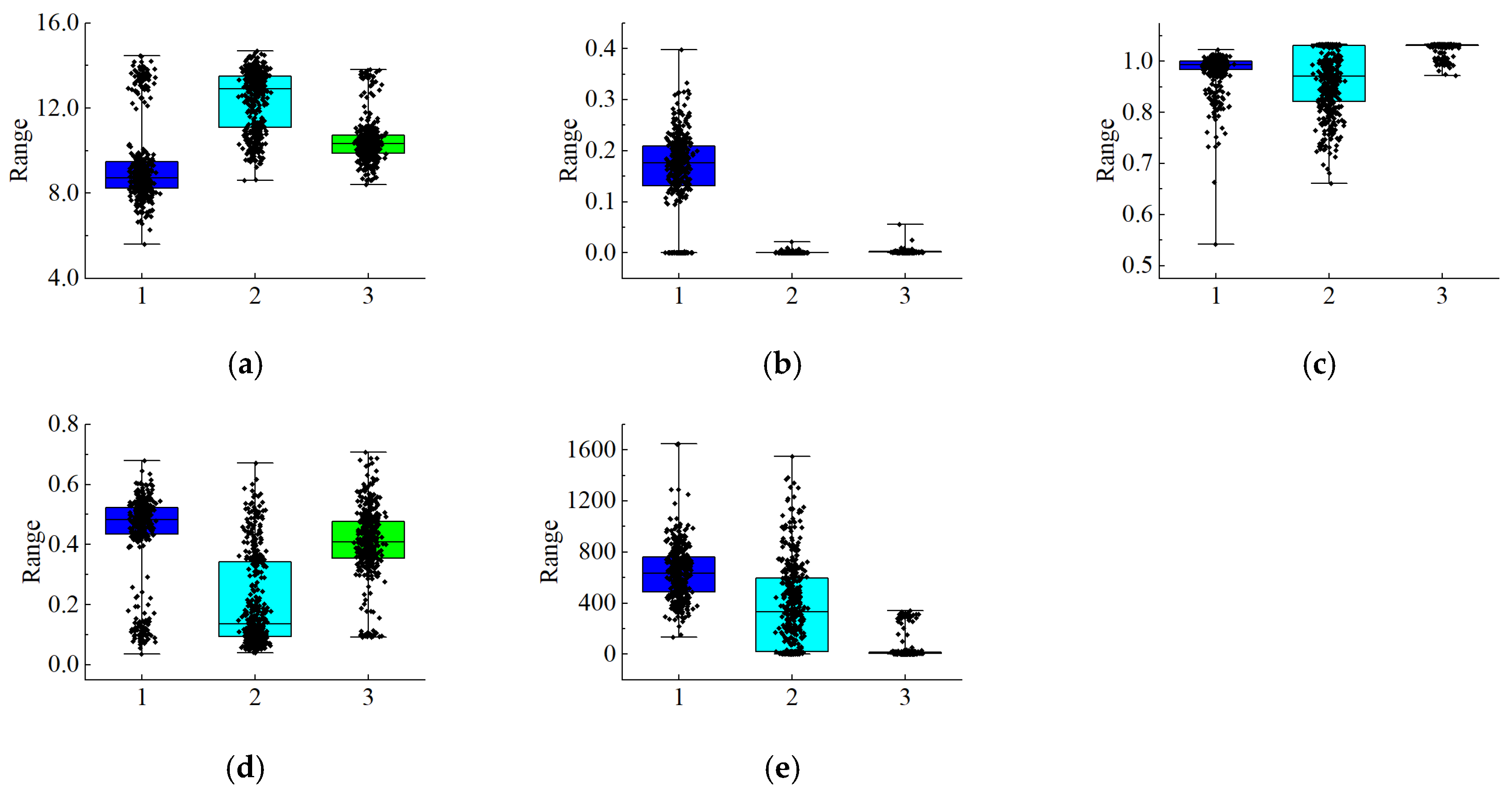
Five typical texture parameters, including entropy, angular second moment (ASM), correlation, inverse difference moment (IDM), and contrast, were extracted based on the gray-level co-occurrence matrix (GLCM). The GLCM was computed at an offset distance of 1 pixel along four directions (0°, 45°, 90°, 135°), and the final texture values were averaged over the four orientations, which kept consistent with the parameter configuration presented in Section 2.2.2. The distribution characteristics of each texture feature are displayed in Figure 7, and the corresponding descriptive statistics are summarized in

Table 4. Statistical results of texture features.

Feature	Bacterial Leaf Spot		Healthy Leaf		Yellow Leaf Curl
	Range	Mean	Range	Mean	Range	Mean
Entropy	5.61~14.48	9.35	8.60~14.68	12.41	8.41~13.80	10.44
Energy	0.00~0.40	0.16	0.00~0.02	0.00	0.00~0.06	0.00
Correlation	0.53~0.99	0.94	0.67~1.00	0.92	0.93~1.00	0.99
Homogeneity	0.04~0.68	0.44	0.04~0.67	0.21	0.09~0.71	0.41
Contrast	135.00~1646.81	637.78	2.50~1548.28	370.03	1.10~341.80	32.13

. All five texture indicators presented obvious inter-group differentiation among the three pepper leaf categories. The mean contrast value of bacterial leaf spot samples reached 637.78, which was considerably higher than that of healthy leaves (370.03) and yellow leaf curl leaves (32.13). Healthy leaves obtained the highest average entropy of 12.41, while yellow leaf curl samples possessed the maximum mean correlation value of 0.99.

3.2.5. Quantitative Feature Screening Based on Random Forest

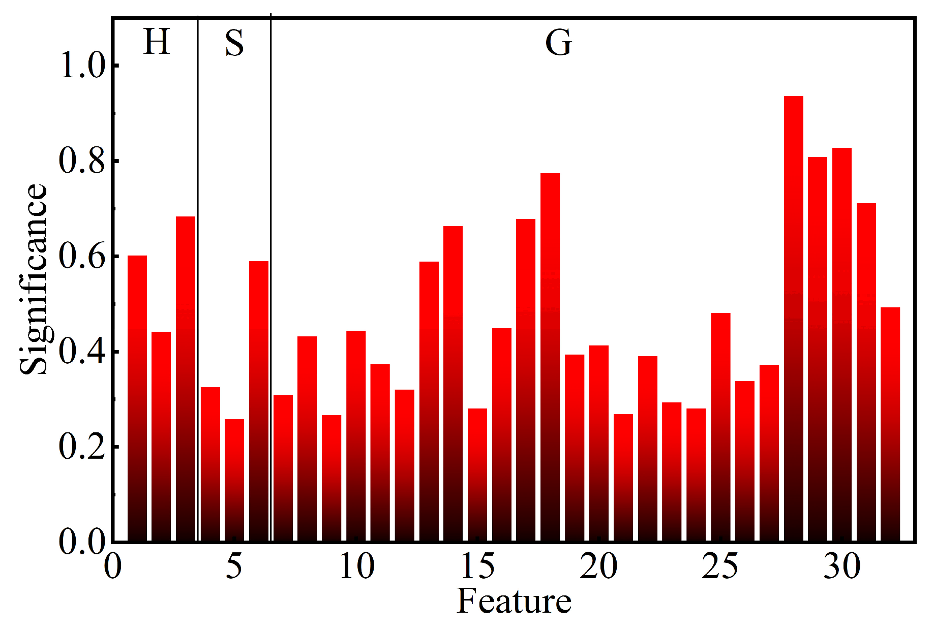
The random-forest classifier was employed to compute the discriminative importance score for each of the 32 fused visual features, and the ranking results are visualized in Figure 8. Feature importance was quantified by the mean decrease in impurity, following the hyper-parameter settings of the random-forest model described in Section 2.2.4. The importance values of Feature 1 to Feature 32 varied between 0.23 and 0.94. Seven features (No. 5, No. 7, No. 9, No. 15, No. 21, No. 23, No. 24) yielded importance scores below the preset threshold of 0.30, indicating weak distinguishing ability and redundant information. After removing these seven low-contribution redundant features, the remaining 25 features with importance values higher than 0.30 were reserved as the optimized input dataset for subsequent classification modeling.

3.3. Construction and Detection Performance of Classification Models

3.3.1. CNN Model

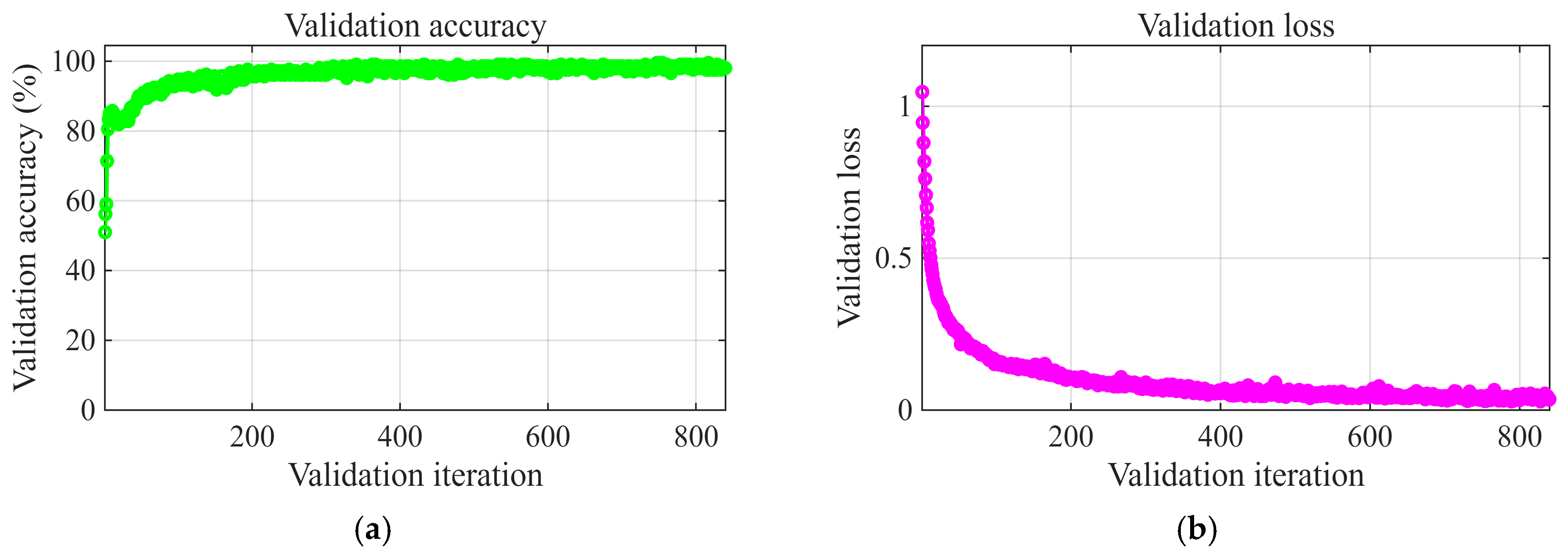
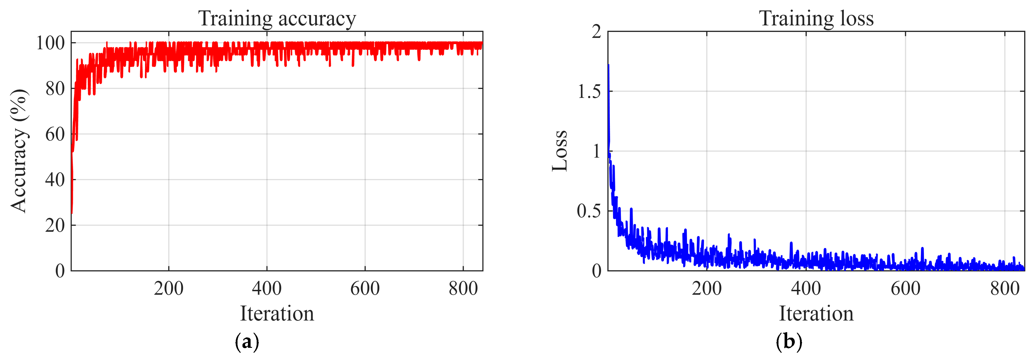
The CNN model was trained for a maximum of 800 epochs, and all hyper-parameters for CNN training remained consistent with the configuration provided in Section 2.2.4. The training accuracy and loss curves, as well as the validation accuracy and loss curves, are illustrated in Figure 9 and Figure 10, respectively. Training accuracy increased steadily during iterative optimization and stabilized above 99% after 735 iterations, while the training loss fluctuated within a very narrow range. The validation metrics exhibited a similar changing trend; validation accuracy reached a stable plateau after 735 iterations, and the validation loss no longer decreased obviously.

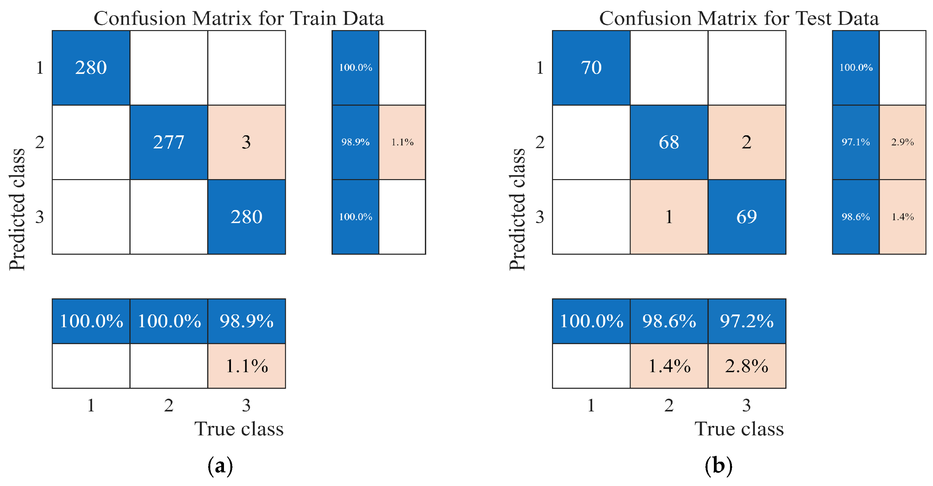
Confusion matrices for the training and test sets of the CNN model are shown in Figure 11, and category-wise quantitative metrics are summarized in

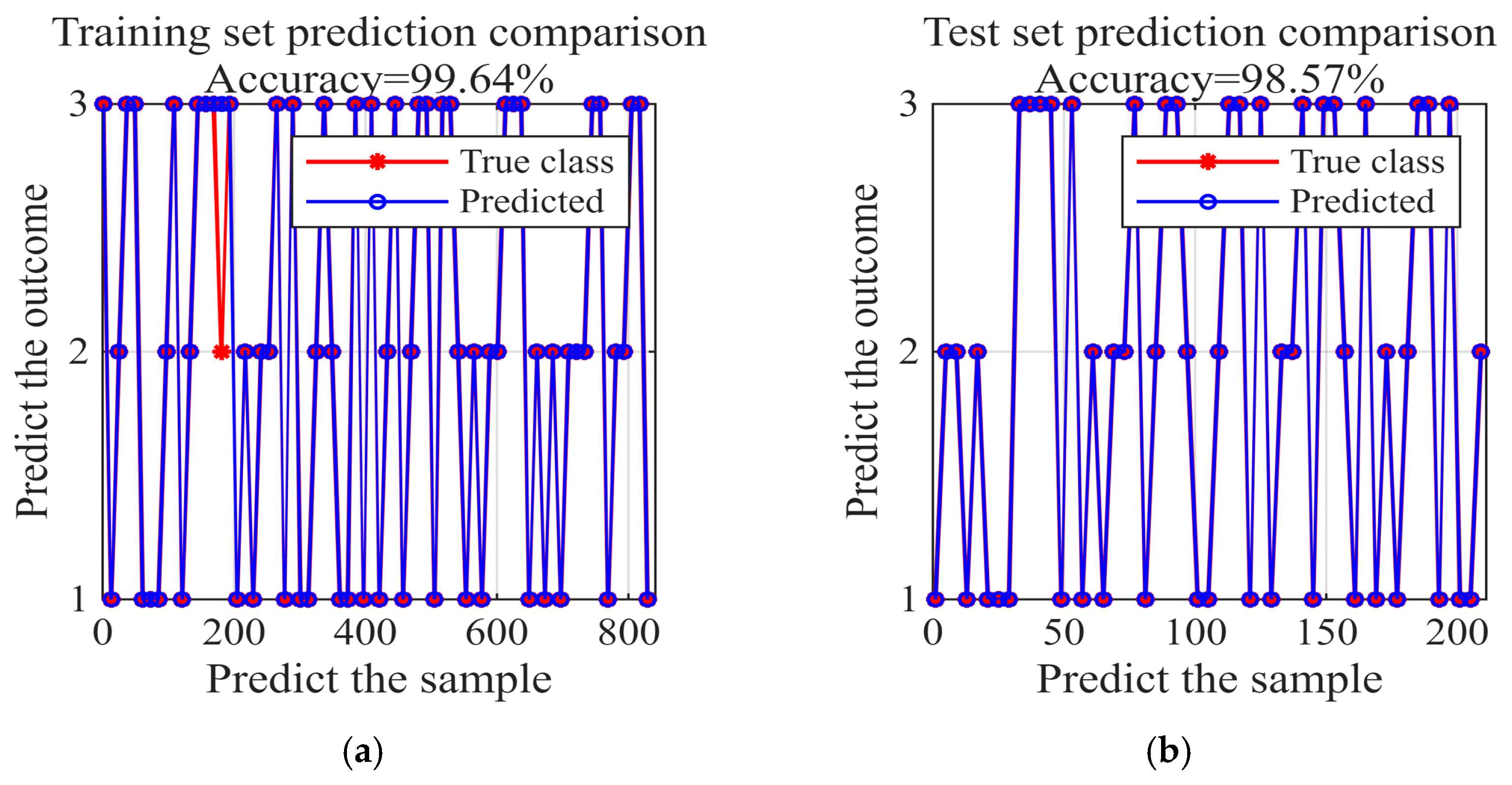
Table 5. The classification metrics of the CNN model on the training and test datasets.

Disease Type	Training Set			Test Set
	Precision	Recall	F1-Score	Precision	Recall	F1-Score
Bacterial leaf spot	100.00	100.00	100.00	100.00	100.00	100.00
Healthy leaf	98.90	100.00	99.45	97.10	98.60	97.84
Yellow leaf curl	100.00	98.90	99.45	98.60	97.20	97.89

. The training set contained 840 samples; all bacterial leaf spot samples were correctly classified, with only three misclassified healthy samples and three misclassified yellow leaf curl samples, yielding an overall training accuracy of 99.64%. The test set included 210 samples with zero misclassifications for bacterial leaf spot, eight misclassified healthy samples, and seven misclassified yellow leaf curl samples, achieving an overall test accuracy of 98.57%. These outcomes correspond to a typical trial selected from 20 independent replicate experiments. 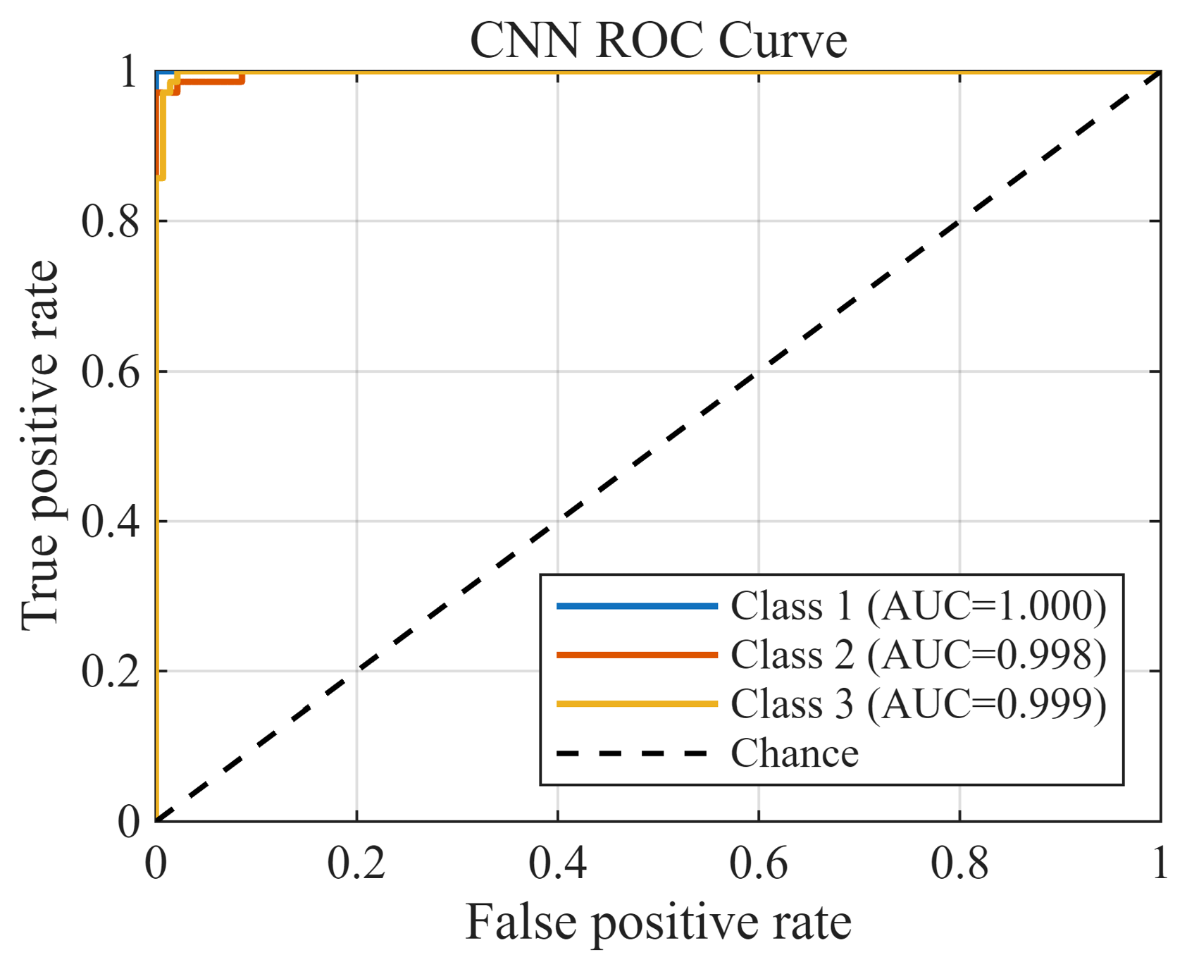Typical prediction results of samples from the training set and test set are presented in Figure 12. The one-versus-rest receiver operating characteristic (ROC) curve of the CNN model (Figure 13) delivered Area Under the Curve (AUC) values of 1.000, 0.998, and 0.999 for the three leaf categories, with all curves tightly close to the top-left corner and far from the random-guess diagonal baseline.

3.3.2. LR Model

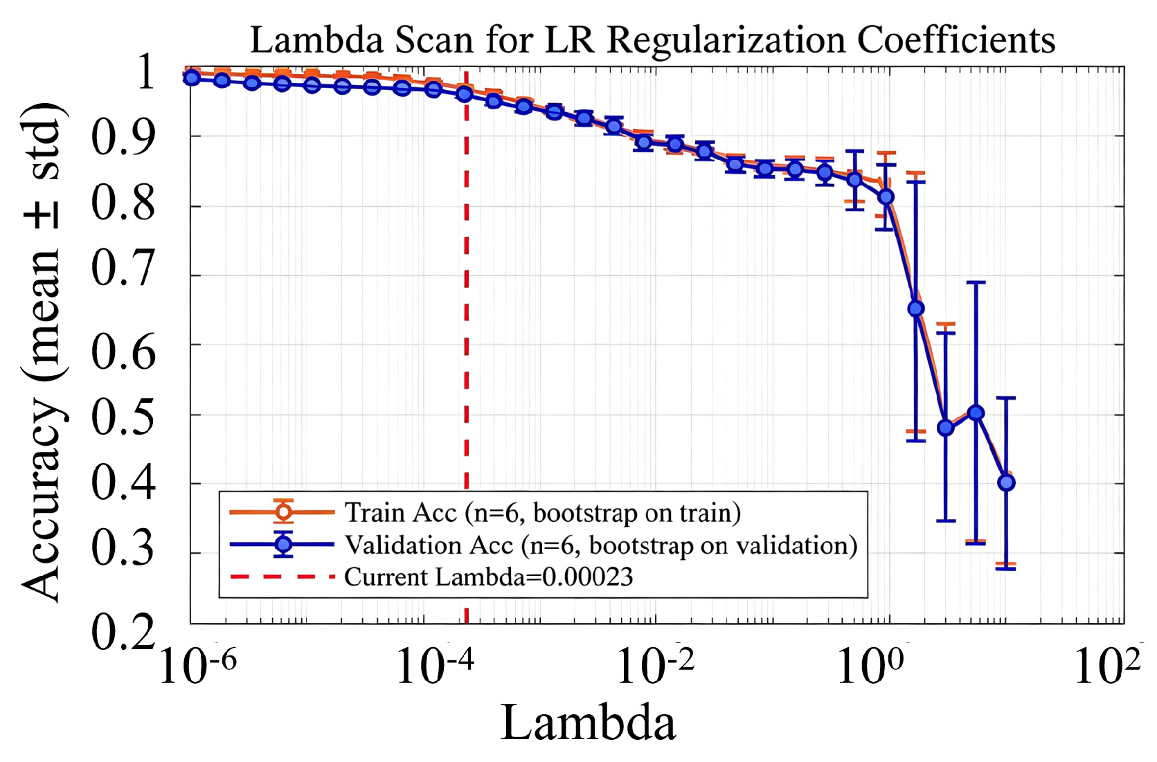
Grid-search optimization was performed for the regularization coefficient λ of the LR model within the range from 10⁻⁶ to 10², and the scanning results are presented in Figure 14. The remaining hyper-parameters of the LR model were kept consistent with the settings described in Section 2.2.4. Training and validation accuracy maintained relatively high and stable values when λ ranged from 10⁻⁶ to 10⁻⁴. The optimal λ was finally set to 0.00023, at which point the accuracy difference between the training and validation sets reached the minimum. Once λ exceeded 0.00023, the validation accuracy dropped rapidly and was accompanied by obvious fluctuations.

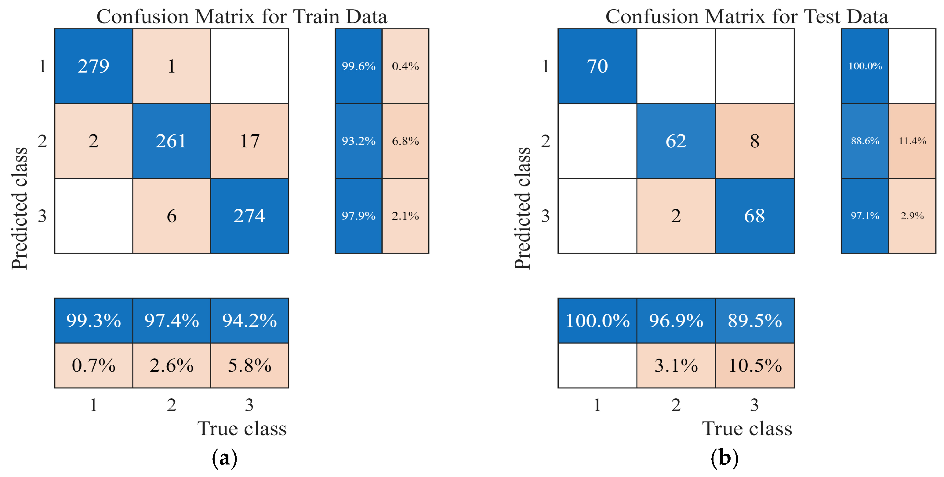
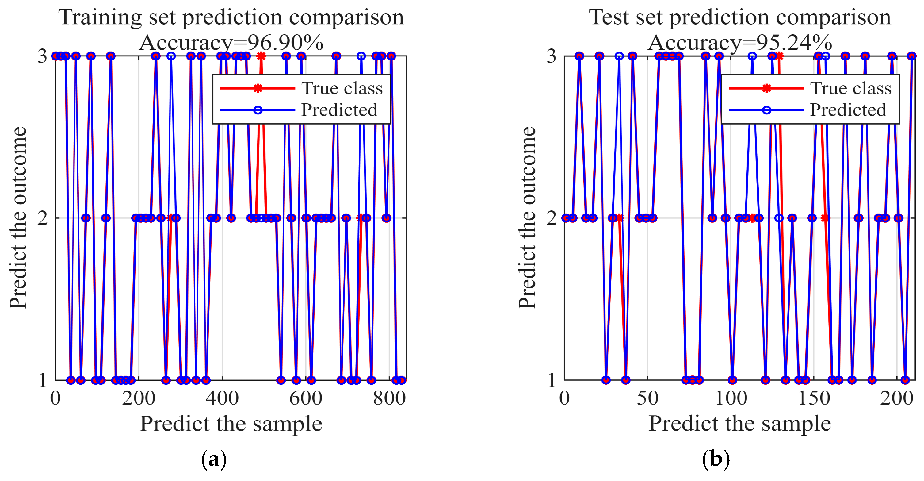
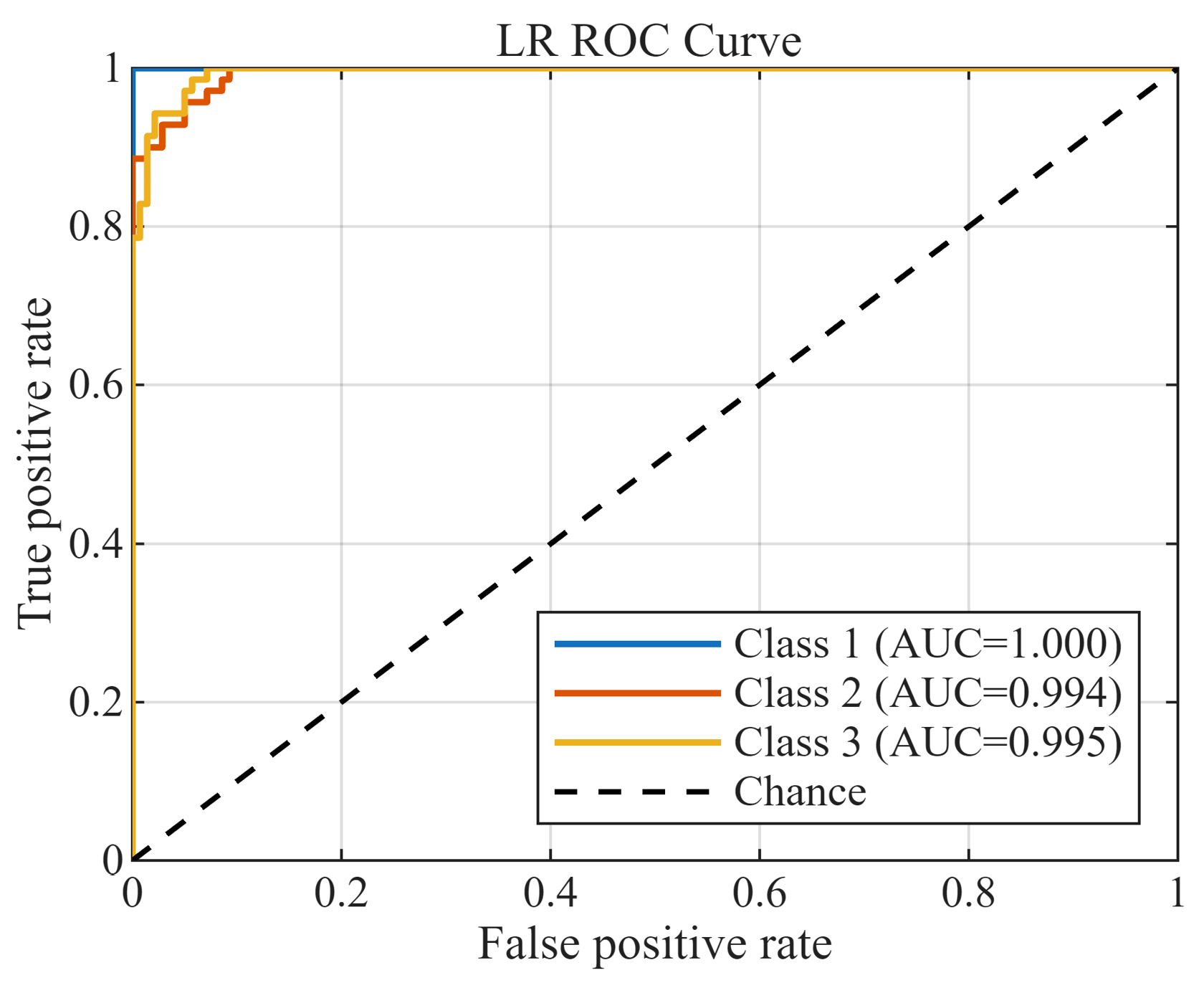
Confusion matrices, sample prediction comparisons, and multi-class receiver operating characteristic (ROC) curves of the LR model are provided in Figure 15, Figure 16 and Figure 17, with quantitative classification metrics listed in

Table 6. The classification metrics of the LR model on the training and test datasets.

Disease Type	Training Set			Test Set
	Precision	Recall	F1-Score	Precision	Recall	F1-Score
Bacterial leaf spot	99.60	99.30	99.45	100.00	100.00	100.00
Healthy leaf	93.20	97.40	95.25	88.60	96.90	92.56
Yellow leaf curl	97.90	94.20	96.01	97.10	89.50	93.15

. These results were obtained from one representative run among the 20 independent replicate experiments. The LR model achieved an overall training accuracy of 96.90%, with minor cross-misclassification between healthy and yellow leaf curl samples, and a test-set accuracy of 95.24% dominated by misclassified healthy leaf samples. The LR ROC curve generated Area Under the Curve (AUC) values of 1.000, 0.994, and 0.995 for the three leaf categories, all lying distinctly above the random-classification diagonal.

3.3.3. GA-BP Model

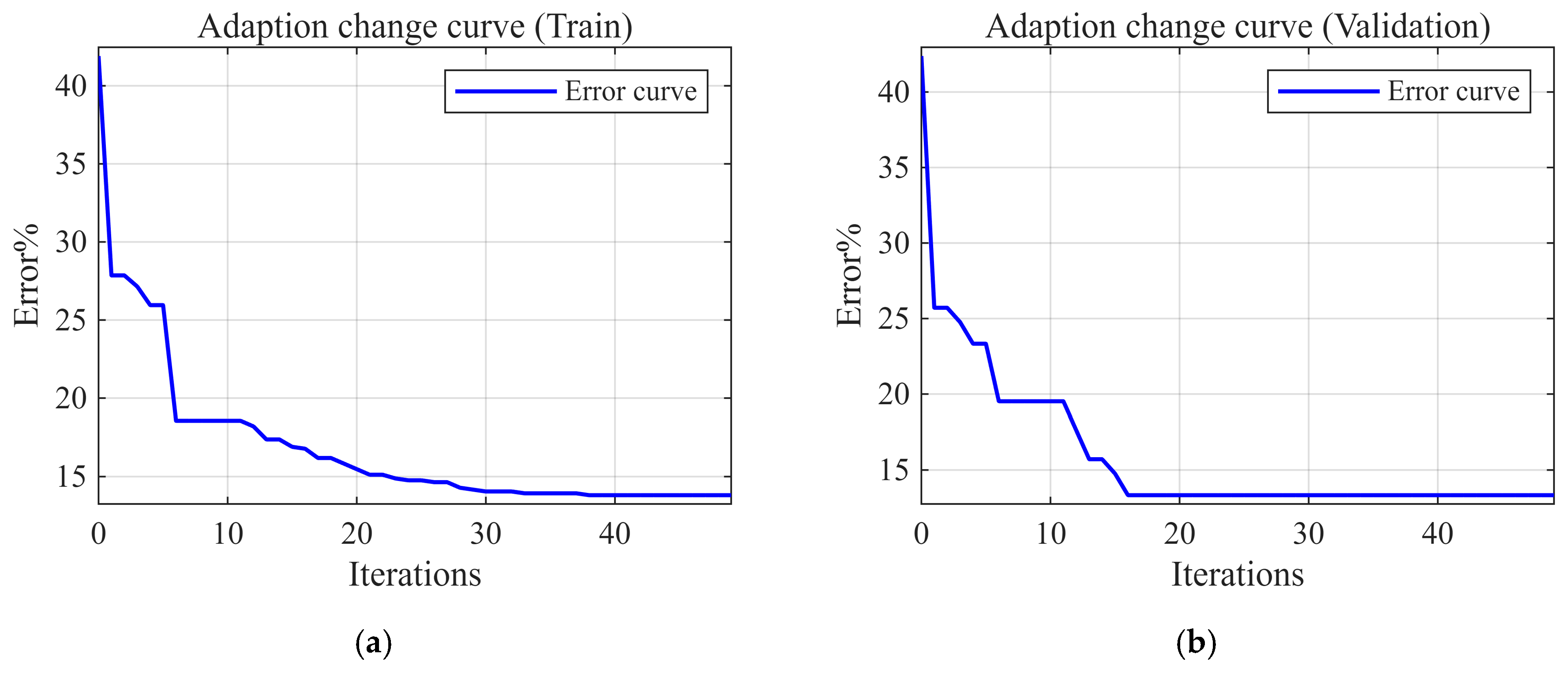
The fitness error curves of genetic optimization for the genetic-algorithm back-propagation (GA-BP) model are presented in Figure 18, and all hyper-parameters of the GA-BP model followed the configuration listed in Section 2.2.4. Both training and validation errors declined continuously within 0–45 genetic iterations and gradually stabilized after 45 iterations. 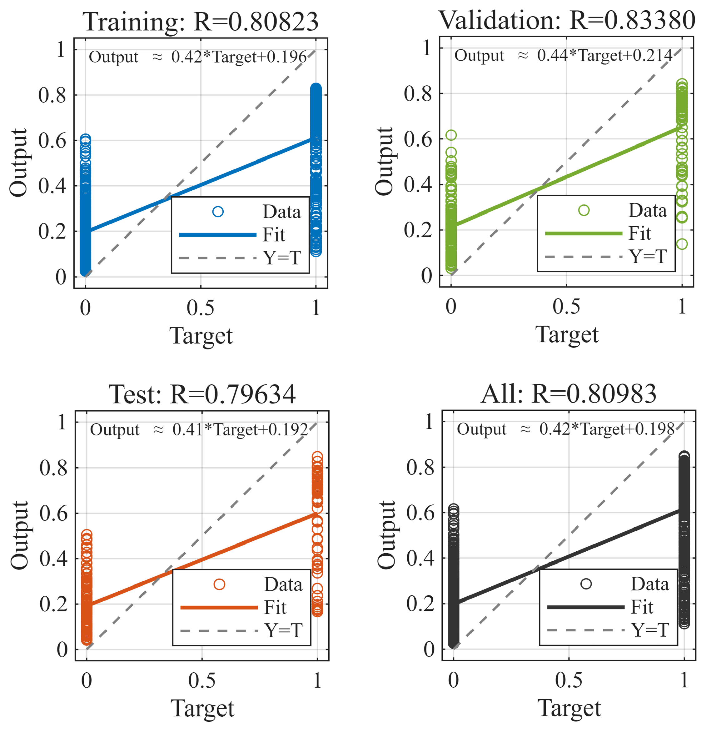The linear regression plots between predicted values and true labels (Figure 19) yielded correlation coefficients R of 0.8082 for the training set, 0.8338 for the validation set, 0.7963 for the test set, and 0.8098 for the full dataset. 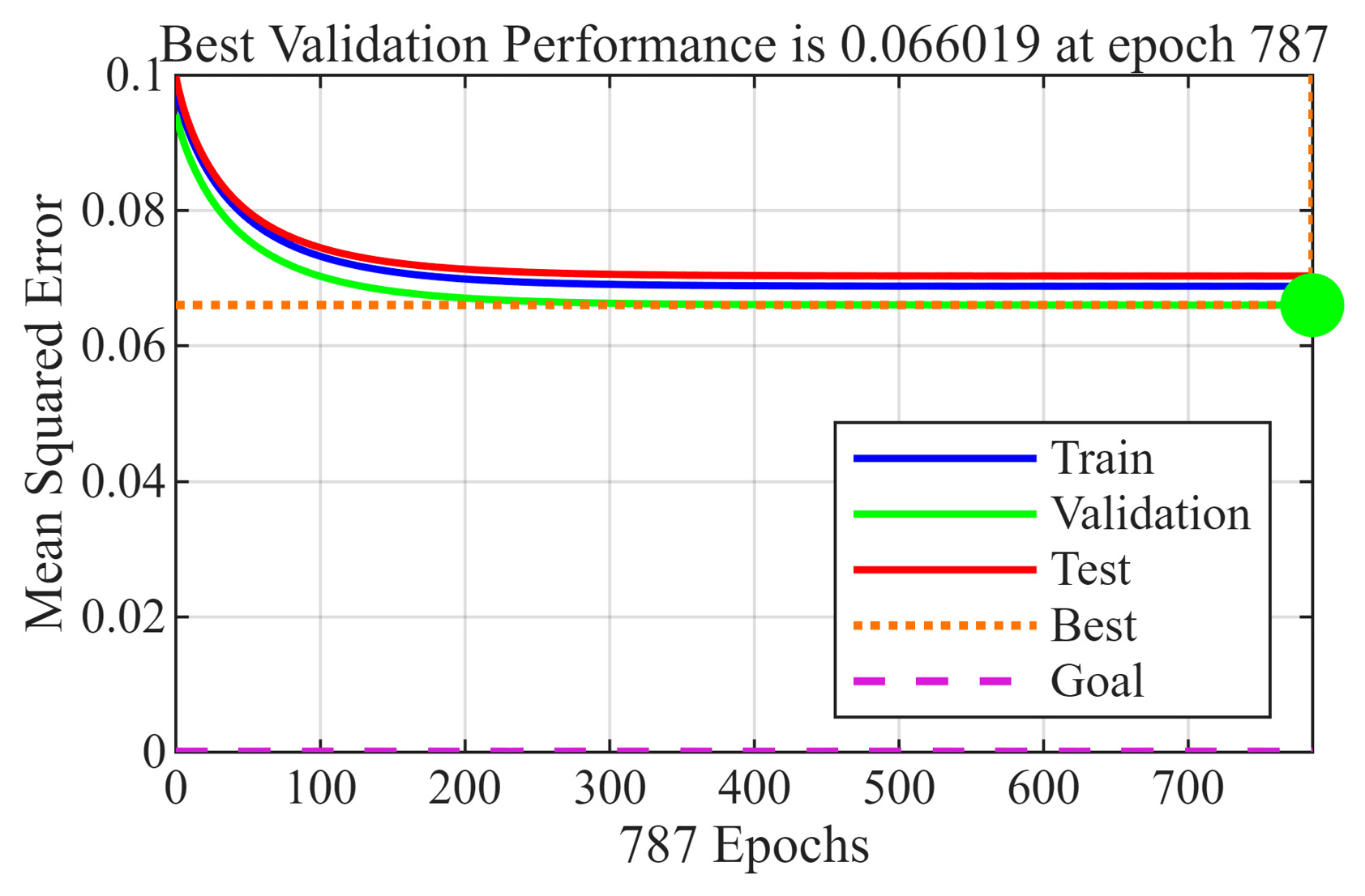The mean squared error (MSE) iteration curve (Figure 20) showed that the minimum MSE value of 0.0660 was obtained at the 787th training epoch, which corresponded to the optimal convergence condition of the neural network.

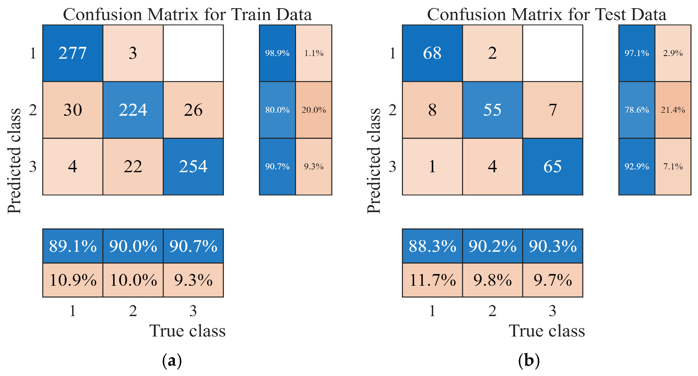
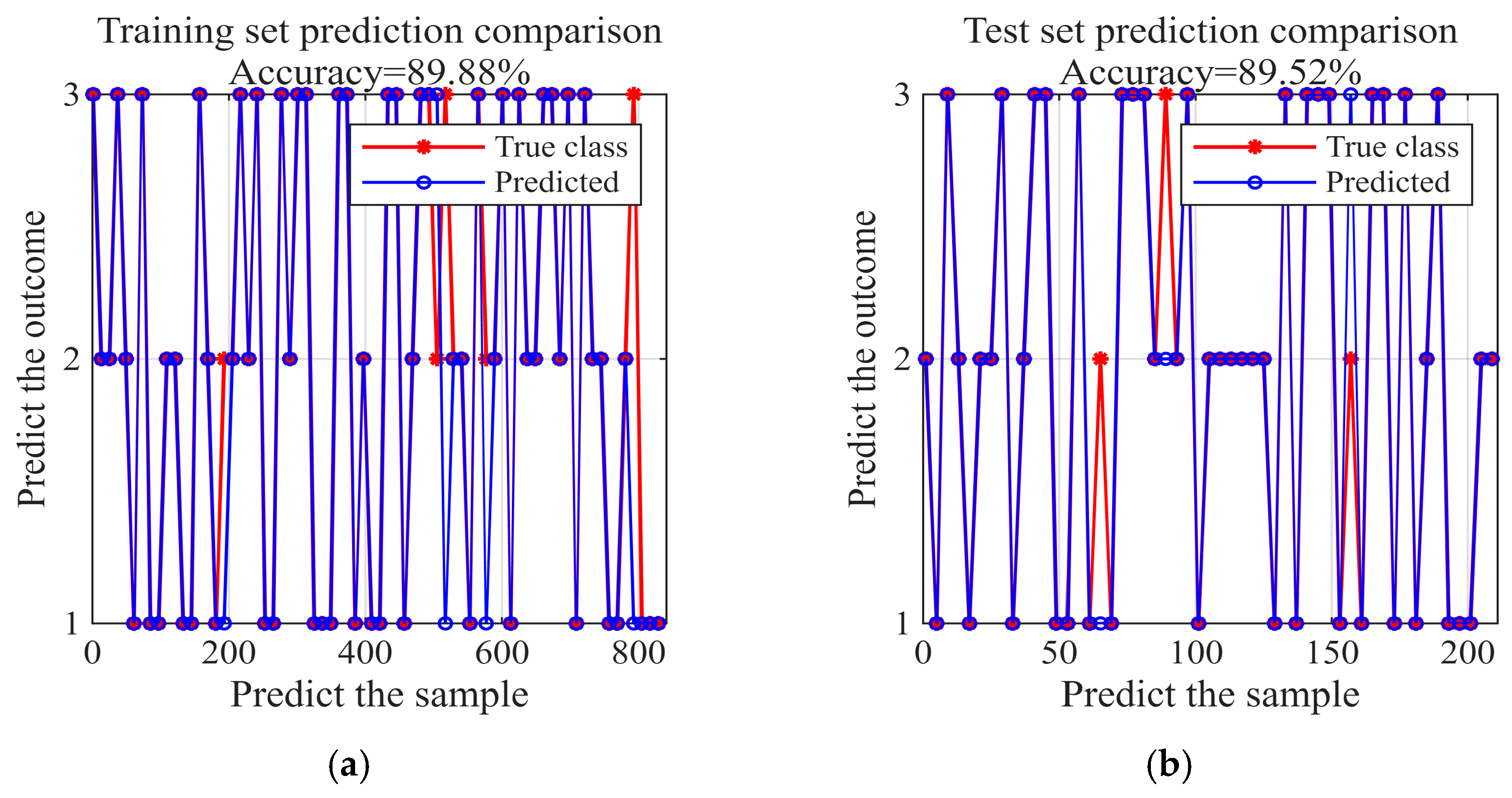
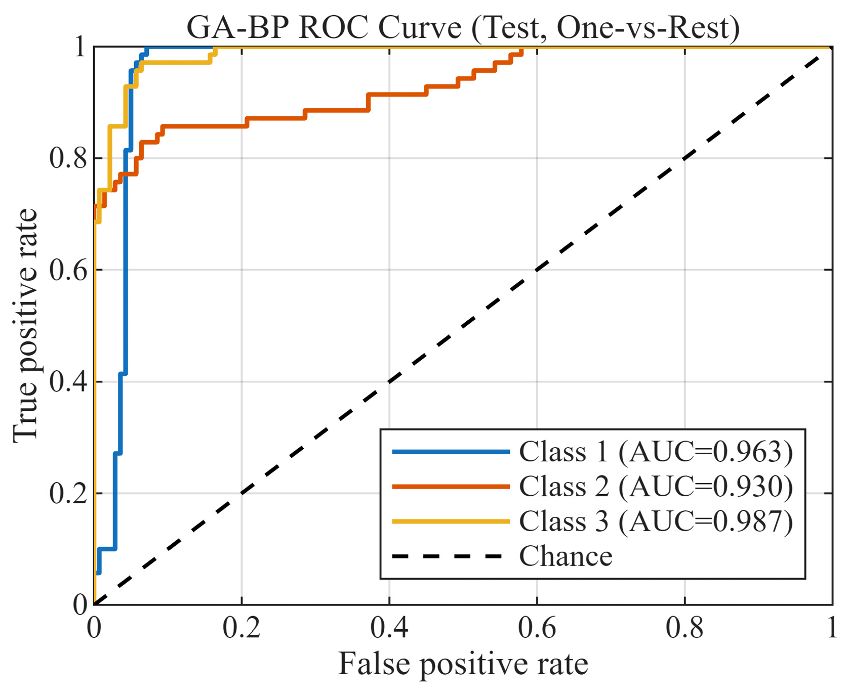
Confusion matrices, sample prediction comparisons, and ROC curves of the GA-BP model are illustrated in Figure 21, Figure 22 and Figure 23, and the corresponding classification metrics are summarized in

Table 7. The classification metrics of the GA-BP model on the training and test datasets.

Disease Type	Training Set			Test Set
	Precision	Recall	F1-Score	Precision	Recall	F1-Score
Bacterial leaf spot	98.90	89.10	93.74	97.10	88.30	92.49
Healthy leaf	80.00	90.00	84.71	78.60	90.20	84.00
Yellow leaf curl	90.70	90.70	90.70	92.90	90.30	91.58

. These classification results were selected as a typical realization from 20 independent replicate runs. The GA-BP model obtained an overall training accuracy of 89.88% (dominated by misclassified healthy leaves) and a test accuracy of 89.52% with frequent cross-category misjudgments across all three leaf types. The one-versus-rest ROC curve produced AUC values of 0.963, 0.930, and 0.987 for bacterial leaf spot, healthy leaves, and yellow leaf curl, respectively. Visible gaps existed between these ROC curves and the ideal top-left corner for perfect classification.

3.3.4. Comprehensive Comparative Analysis of Three Classification Models

Each classification model was run for 20 independent replicates. Descriptive statistical results of evaluation metrics on the training set are summarized in

Table 8. Statistics of 20 running results for training set.

Model	Recall			F1-Score			Accuracy
	Range	Mean	Std.	Range	Mean	Std.	Range	Mean	Std.
CNN	98.09~99.88	99.32	0.0045	98.03~99.88	99.31	0.0046	97.98~99.88	99.30	0.0047
LR	96.48~97.36	96.88	0.0025	96.46~97.31	96.85	0.0024	96.43~97.26	96.82	0.0024
GA-BP	81.18~92.68	88.14	0.0273	81.31~92.53	88.10	0.0274	81.43~92.50	88.05	0.0275

, while those for the test set are listed in

Table 9. Statistics of 20 running results for test set.

Model	Recall			F1-Score			Accuracy
	Range	Mean	Std.	Range	Mean	Std.	Range	Mean	Std.
CNN	95.45~99.53	97.71	0.0102	95.34~99.53	97.69	0.0103	95.24~99.52	97.67	0.0104
LR	94.14~98.58	96.65	0.0111	93.97~98.57	96.60	0.0114	93.81~98.57	96.55	0.0117
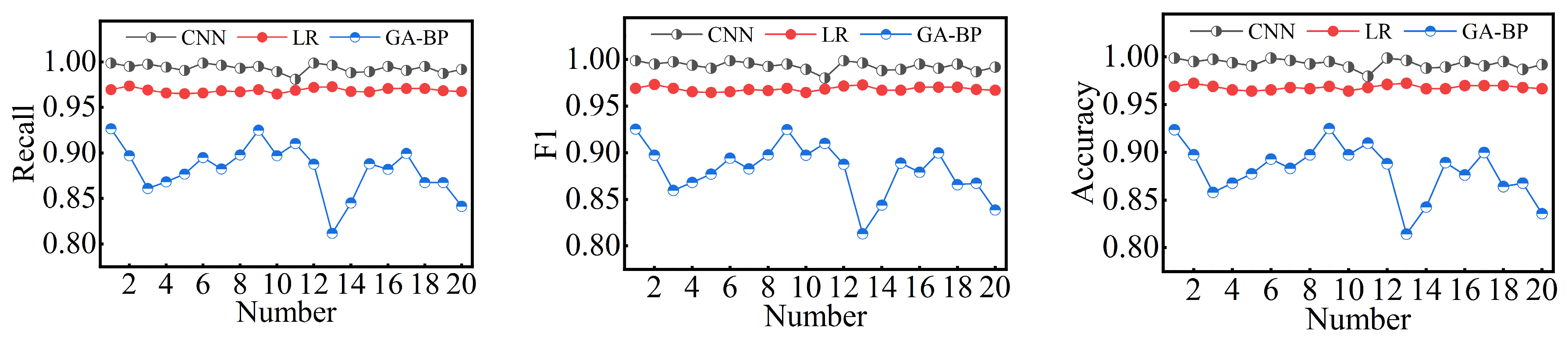
GA-BP	82.35~92.31	88.03	0.0274	81.89~92.11	87.91	0.0280	81.43~91.90	87.78	0.0287

. Across the 20 repeated training set trials, the CNN model achieved a mean macro-recall of 99.32%, a mean macro-F1-score of 99.31%, and a mean accuracy of 99.30%, with the standard deviations of all three metrics lower than 0.005. The LR model presented intermediate mean values for all indicators between CNN and GA-BP, accompanied by standard deviations below 0.003. By contrast, the GA-BP model obtained the lowest mean performance values among the three approaches, with standard deviations exceeding 0.027. For the test-set evaluations over 20 replicates, the CNN yielded a mean macro-recall of 97.71% and a mean accuracy of 97.67%, with a standard deviation of 0.0104. The LR model reached a mean test-set accuracy of 96.55% and a standard deviation of 0.0117. The GA-BP model had a mean test-set accuracy of 87.78% with the highest standard deviation (0.0287) of the three models. A smaller standard deviation represents more stable generalization performance of the model. The changes in recall, F1-score and accuracy across the 20 replicates of the three models are visualized in Figure 24.

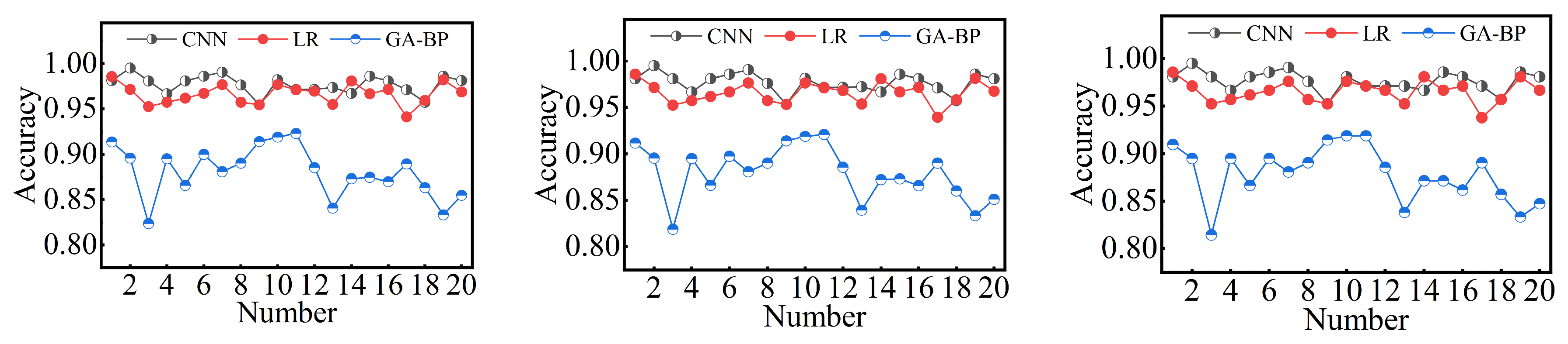
The detection results on the test set (see Figure 25 and Table 9) indicate that the GA-BP model exhibits the largest standard deviation in precision, recall, and accuracy, followed by the LR model, while the CNN model demonstrates the smallest standard deviation. Further test-set performance comparison indicated that both the LR algorithm and the CNN neural network achieved comparable recognition accuracy, and both significantly outperformed the GA-BP neural network model.

4. Discussion

The experimental results of this study demonstrated that the Lab b-channel-based background segmentation method outperformed the RGB super-green feature method and the Otsu-ACWE model for pepper leaf image preprocessing. The RGB super-green and Otsu-ACWE segmentation approaches were only used for comparative evaluation in Section 3.1; owing to its superior preservation of lesion boundaries, only the Lab b-channel segmentation pipeline was adopted for subsequent feature extraction. Benefiting from the perceptual uniformity of the Lab color space, this method effectively enhanced the chromatic contrast between green leaf tissues and complex field backgrounds, while preserving subtle lesion boundary details through morphological postprocessing, thereby providing a reliable basis for subsequent color and texture feature extraction.

In total, 32 fused visual features were extracted in this work, comprising 27 color moment features from the RGB, HSV and Lab color spaces and five texture features derived from the gray-level co-occurrence matrix (GLCM). GLCM texture features were computed at an offset distance of one pixel along four orientations (0°, 45°, 90°, 135°) and averaged across directions to generate stable texture descriptors. Quantitative feature importance analysis using the random-forest classifier showed that seven features with low discriminative contribution introduced redundant computational cost without improving classification performance. These redundant features were removed using a fixed importance threshold of 0.30, and the remaining 25 informative features were retained to balance feature dimensionality and model recognition accuracy.

The statistical distributions of feature values revealed that the first-order moments of the three color spaces exhibited clear inter-class differentiation among healthy leaves, bacterial leaf spot leaves and yellow leaf curl leaves, whereas some second- and third-order moments showed substantial overlap across categories, accounting for their low feature importance. In addition, GLCM-based texture metrics (e.g., entropy and contrast) provided complementary discriminative information to color features, effectively differentiating leaf samples with similar coloration but distinct lesion texture patterns.

The performance differences among the CNN, LR and GA-BP models were inherently determined by their respective algorithmic architectures. All model comparisons were conducted based on 20 independent replicate experiments with fixed random seeds to reduce random errors and ensure statistical reliability. As an end-to-end deep-learning framework, the CNN automatically extracted high-level semantic lesion features through stacked convolutional and pooling layers, achieving an average test accuracy of 97.67% and the smallest standard deviations of evaluation metrics across the 20 replicate trials, which verified its superior classification accuracy and robustness. The linear LR model performed multi-class classification using the ECOC strategy based on manually screened shallow visual features, exhibiting moderate recognition performance and low computational overhead.

Although the genetic algorithm optimized the initial weights and biases of the BP neural network to mitigate local optima, the GA-BP model still suffered from limited nonlinear fitting capability and high sensitivity to random initialization and dataset partitioning. This resulted in the lowest average test accuracy (87.78%) and the largest fluctuations in evaluation metrics, which limited its applicability for high-precision pepper leaf disease detection.

Compared with existing related studies that only employed single preprocessing strategies, single-feature sources, or a limited number of comparative models, this work established a standardized experimental pipeline encompassing multi-algorithm background segmentation, multi-modal feature fusion, quantitative feature screening, and three representative classification models. Furthermore, replicate experiments were conducted to reduce random errors arising from dataset splitting and model initialization, thereby improving the objectivity and reliability of the experimental conclusions.

Nevertheless, several limitations should be acknowledged in the current study. First, the dataset only includes three leaf categories without covering other common pepper diseases, and all images were acquired under uniform lighting conditions, which may restrict the generalization performance of the models in complex field environments. Second, only shallow color and texture features were used, and morphological and edge features were not incorporated, which limits the identification of early-stage lesions with subtle visual symptoms. Third, the vanilla CNN model has relatively high computational resource requirements.

Future work will expand the dataset by including more disease categories and multi-scene leaf images acquired under varying illumination conditions and across different growth stages. Multi-modal visual features, such as leaf contour and fractal dimension, will be fused with attention mechanisms to enhance the recognition capability for early-stage mild diseases. Lightweight network architectures and model compression techniques will be employed to reduce the parameter size and computational cost of the CNN model. Furthermore, environmental factors (e.g., field temperature, humidity, and soil conditions) will be integrated to construct a multi-source fusion diagnosis model, enabling simultaneous disease identification, severity grading, and outbreak risk prediction. This will provide more comprehensive technical support for the intelligent plant protection of pepper crops.

5. Conclusions

This study selected healthy pepper leaves, leaves infected with bacterial leaf spot, and leaves with yellow leaf curl as research materials, and constructed a standardized experimental workflow for pepper leaf disease recognition based on computer vision and machine learning. A complete experimental pipeline was established, including multi-algorithm image segmentation, multi-modal visual feature fusion, quantitative feature screening, and heterogeneous multi-model comparative evaluation. The main conclusions are summarized as follows:

The Lab-b-channel segmentation algorithm yielded an average IoU value of 0.942 and well preserved fine lesion boundaries, achieving better foreground extraction performance than the RGB super-green method and the Otsu-ACWE segmentation model. The fused feature set integrating color moments from RGB, HSV and Lab spaces as well as GLCM texture features can sufficiently capture the visual differences among the three categories of pepper leaf samples. GLCM texture features were calculated with a one-pixel offset along four orientations (0°, 45°, 90°, 135°), and the directional results were averaged to obtain robust texture descriptors. According to the feature importance ranking derived from the random-forest classifier, seven redundant features with importance scores lower than the preset threshold of 0.30 were discarded. This strategy reduced the computational overhead of subsequent classification models without degrading discriminative capability. All color features were computed following unified statistical definitions: the first-order moment (mean value), the second-order moment (standard deviation), and the third-order moment (skewness).

Obvious performance differences were observed among the CNN, LR and GA-BP models, with the overall performance ranked as CNN > LR > GA-BP. Fixed random seeds and 20 independent replicate runs were adopted for all model evaluations to guarantee experimental reproducibility. Over the 20 repeated tests, the CNN model achieved an average test accuracy of 97.67% and an average AUC of 0.999, together with the minimum standard deviation across all evaluation metrics, demonstrating its superior classification accuracy and stability. The LR model had fewer parameters and faster inference speed. The GA-BP model introduced a genetic algorithm to optimize the initial weights and biases of the BP neural network for alleviating local optima. Nevertheless, the GA-BP network was constrained by insufficient nonlinear fitting ability and substantial prediction fluctuation, which made it unsuitable for high-precision field-based pepper disease diagnosis.

Carrying out multiple independent replicates and quantifying model stability using standard deviation helps reduce random errors originating from dataset partitioning and random weight initialization in a single run. Combined with one-way ANOVA significance analysis, the reliability and reproducibility of the experimental conclusions were effectively enhanced. Stratified random sampling was employed to split the dataset, maintaining balanced class proportions among the training, validation and test subsets.

The standardized experimental framework proposed in this work offers a unified reference for image preprocessing, feature engineering and multi-model comparison in vegetable leaf disease detection. It can provide theoretical foundations and empirical evidence for algorithm screening and experimental design in intelligent disease diagnosis for pepper and other high-value vegetable crops.