Non-Destructive Three-Dimensional Phenotyping of Garlic Bulbs Based on Multi-View Imaging

Highlights

What are the main findings?

• A grading-oriented, non-destructive 3D phenotyping workflow was developed for garlic bulbs using multi-view imaging and point cloud processing.
• The workflow enabled accurate extraction of maximum longitudinal diameter, maximum transverse diameter, and bulb volume.
• The extracted traits showed strong agreement with manual measurements, with R² values of 0.9935, 0.9909, and 0.9924 for longitudinal diameter, transverse diameter, and volume, respectively.

What are the implications of the main findings?

• This study establishes a reproducible image-based three-dimensional measurement workflow for garlic bulb phenotypic analysis and validates its performance under controlled laboratory conditions.
• The workflow offers a practical reference for 3D phenotyping and post-harvest grading of bulbous horticultural crops.

Abstract

Traditional manual measurement of garlic bulb phenotypic traits is inefficient, subjective, poorly reproducible, and may cause sample damage. To improve the adaptability of three-dimensional reconstruction to garlic bulb morphology and grading-related parameter extraction, this study developed a non-destructive phenotypic measurement workflow based on multi-view image-based three-dimensional reconstruction. Four garlic materials with distinct bulb morphologies and epidermal characteristics were used to demonstrate the feasibility of the reconstruction workflow, and 40 Lanling white-skinned garlic bulbs were used for quantitative accuracy validation. Multi-view images were acquired using a high-resolution camera, a motorized turntable, and a controlled illumination system. Three-dimensional models were reconstructed using ContextCapture, and the resulting point clouds were processed in CloudCompare through cropping, denoising, downsampling, and pose correction. Maximum longitudinal diameter, maximum transverse diameter, and volume were extracted from the processed point clouds according to GB/T 45244-2025 (Grades and Specifications of Garlic) and validated against manual reference measurements. The coefficients of determination for maximum longitudinal diameter, maximum transverse diameter, and volume were 0.9935, 0.9909, and 0.9924, respectively, with RMSE values of 0.0529 cm, 0.0520 cm, and 0.8874 cm³, and MAPE values of 0.6647%, 0.7765%, and 1.9149%. Additional MAE, bias, confidence interval, and Bland–Altman analyses further supported the agreement between model-derived and manual reference measurements. These results demonstrate the feasibility of multi-view image-based three-dimensional reconstruction for non-destructive garlic bulb phenotypic measurement and provide a methodological basis for future grading-related assessment and three-dimensional phenotyping of bulbous horticultural crops.

1. Introduction

Garlic is a globally important crop with both medicinal and culinary uses [1], and it has considerable economic value in vegetable production, condiment processing, and the development of functional foods [2]. China is one of the world’s major garlic producers and exporters [3]. According to forecasts released in March 2026 by the Garlic Market Analysis and Early Warning Team of the Ministry of Agriculture and Rural Affairs, China’s garlic cultivation area is projected to reach 12.83 million mu in 2026, with total production of 15.99 million tonnes, and the country is expected to remain the world’s largest garlic producer and exporter in the long term. The external morphological and structural traits of garlic bulbs, such as bulb diameter and volume, directly influence commercial grade, processing suitability, and yield potential, and are therefore key phenotypic indicators for garlic breeding evaluation and post-harvest grading [4].

Phenomics serves as a bridge between genotype and environment and has become a key enabling technology for crop breeding, cultivation management, and germplasm evaluation. Early studies on three-dimensional crop phenotyping mainly relied on active sensing or tomographic imaging technologies, including LiDAR, structured light scanning, CT/MRI, and micro-CT. LiDAR can directly acquire three-dimensional point clouds of crop canopies or individual plants and has important applications in the analysis of plant height, canopy height, tiller number, and population structure. Friedli et al. used ground-based 3D laser scanning to monitor dynamic changes in canopy height in wheat, maize, and soybean, demonstrating the feasibility of TLS for acquiring crop canopy phenotypes [5]. Based on ground-based LiDAR data, Fang et al. achieved non-destructive and automated estimation of tiller number in field-grown wheat [6]. Structured light technology has also been used for plant 3D reconstruction and for extracting phenotypic parameters such as plant height, leaf number, leaf size, and internode length [7]. Micro-CT is primarily used for the 3D visualization of internal plant structures, enabling the analysis of internal phenotypic traits in seeds, root systems, stem and leaf tissues, vascular tissues, and air-space structures [8].

Although active sensing and tomographic imaging technologies can generate high-quality 3D data, their application in large-scale crop phenotyping remains limited by high equipment costs, complex operational procedures, limited environmental adaptability, and low detection efficiency. LiDAR data processing typically involves point cloud registration, denoising, segmentation, and parameter extraction, which places high demands on acquisition conditions, operational expertise, and computational resources. Structured light scanning is susceptible to natural illumination, target movement, and occlusion; therefore, it is more suitable for indoor or relatively stable environments. Although micro-CT can non-destructively capture internal plant structures, it is constrained by high equipment costs, limited sample size, and low scanning efficiency, making it difficult to meet the requirements of large-scale, high-throughput, and low-cost detection in field or post-harvest settings. Therefore, developing low-cost and easily deployable 3D phenotyping methods for large-scale detection is of considerable practical importance.

In recent years, vision-based 3D reconstruction has gradually emerged as an important direction in crop 3D phenotyping because of its low cost, non-destructive nature, ease of use, and broad applicability [9]. Lou et al. were among the first to use consumer-grade cameras to acquire multi-view images and combine SfM with stereo matching for plant 3D reconstruction, demonstrating the feasibility of conventional image-based 3D reconstruction for low-cost plant phenotyping [10]. Subsequently, Duan et al. used multi-view images and VisualSFM software to reconstruct the 3D structure of wheat seedlings and extract parameters such as plant height, leaf length, leaf angle, and tiller number [11]. Zhang et al. applied a single-camera multi-view SfM method to reconstruct sweet potato plants and monitor their growth parameters under field conditions [12]. Wang et al. proposed 3DPhenoMVS, a low-cost 3D phenotyping workflow for tomato, and successfully extracted multiple phenotypic traits from both plants and fruits [13]. Based on a multi-view automated imaging system, Li Baiming et al. optimised 3D point cloud reconstruction strategies for different crops and growth stages, providing a methodological reference for high-quality crop point cloud acquisition and parameter extraction [14].

However, the application of vision-based 3D reconstruction to garlic phenotyping remains limited. First, existing garlic phenotyping methods are constrained by low detection efficiency, limited non-destructiveness, and insufficient scalability, making it difficult to meet the requirements of post-harvest grading, large-scale germplasm screening, and industrial quality assessment. Second, existing 3D modelling methods are mainly optimised for plant architecture or canopy morphology in gramineous crops such as wheat, rice, and maize, and they are poorly adapted to bulbous organs such as garlic bulbs. Garlic bulbs have fine skin texture, complex scale boundaries, localised depressions, folds, and irregular contours. These characteristics can lead to missing surface details, incomplete edge contours, and local voids in reconstructed point clouds, thereby reducing the accuracy of key phenotypic parameter extraction. Moreover, although GB/T 45244-2025, Grading Specifications for Garlic, provides a standard basis for garlic grade classification [15], automated methods for extracting 3D phenotypic parameters according to these grading requirements remain lacking.

To address these research gaps, this study aimed to develop a non-destructive three-dimensional phenotyping workflow for garlic bulbs based on multi-view imaging and point-cloud processing. Specifically, the objectives were to (1) establish a standardized image acquisition and photogrammetric reconstruction procedure for garlic bulbs; (2) extract key grading-related phenotypic parameters, including maximum transverse diameter, maximum longitudinal diameter, and volume, from reconstructed point clouds according to GB/T 45244-2025 [15]; and (3) validate the model-derived measurements against manual reference measurements. This study was designed to provide a methodological basis for the automated phenotypic measurement of bulbous crops.

2. Materials and Methods

2.1. Experimental Equipment and Materials

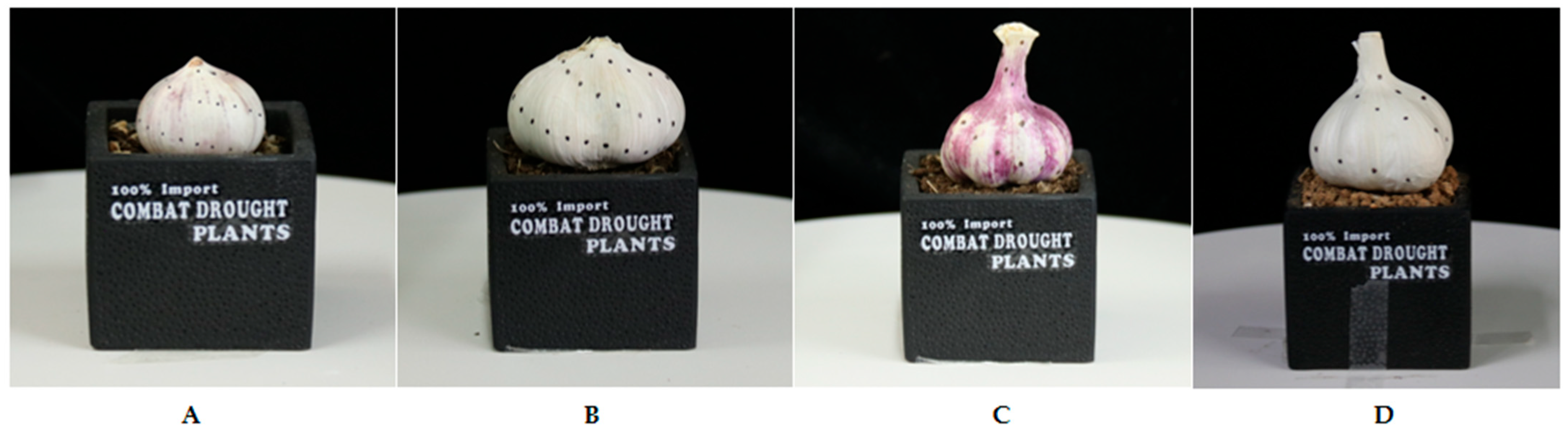
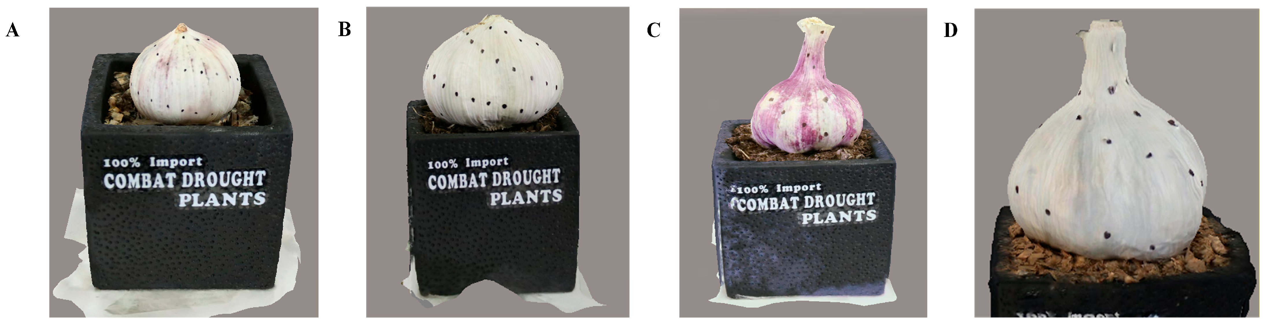
Four garlic materials with distinct bulb morphologies and epidermal characteristics were selected in this study, including Pizhou single-clove garlic (Figure 1A), Pizhou white-top garlic (Figure 1B), Yunnan purple-skinned garlic (Figure 1C), and Lanling white-skinned garlic (Figure 1D). These materials were used to demonstrate the feasibility of the multi-view imaging and three-dimensional reconstruction workflow for garlic bulbs with different external characteristics. For the feasibility demonstration, representative bulb samples from each garlic material were reconstructed, and one typical three-dimensional model of each material was presented as an example.

Among the four materials, Lanling white-skinned garlic was selected as the representative material for quantitative accuracy validation. A total of 40 Lanling white-skinned garlic bulbs were used for paired comparison between manual reference measurements and model-derived phenotypic parameters. All validation samples were mature, healthy, undamaged, mould-free, and non-sprouted. Bulbs with severe mechanical damage, missing cloves, obvious deformation, abnormal sprouting, or heavy surface contamination were excluded. To represent the natural size variation within Lanling white-skinned garlic, bulbs of different sizes were included. The manually measured longitudinal diameter, transverse diameter, and volume of the 40 validation samples ranged from 5.53 to 7.57 cm, 4.63 to 6.38 cm, and 21.56 to 59.18 cm³, respectively.

The experiment was conducted in 2025 at the Shandong Provincial Key Laboratory of Smart Production Technology and Equipment for Protected Horticulture. Auxiliary materials included a matte black background cloth, standard calibration blocks, fixed sample pots, and lightweight ballast, which were used to reduce image glare, ensure accurate scale calibration, and maintain sample stability during image acquisition.

The experimental equipment mainly consisted of a Canon EOS 80D high-resolution digital camera equipped with a Canon EF-S 18–135 mm lens (Canon Inc., Tokyo, Japan), a timer shutter release cable, an MT-380 high-precision motorized indexing turntable (Shenzhen ComXim Technologies Co., Ltd., Shenzhen, China), a Godox SL60 LED continuous light source (Godox Photo Equipment Co., Ltd., Shenzhen, China), a height-adjustable image acquisition stand, and a Dell laptop (model, Dell Technologies Inc., Round Rock, TX, USA), which together enabled uniform illumination, multi-view image acquisition, and controlled sample rotation. Data processing was performed on a high-performance computer workstation. The experimental software included TurntableX-1.5.4 (Shenzhen ComXim Technologies Co., Ltd., Shenzhen, China) for motorized turntable control and multi-view image acquisition, ContextCapture Center 64-bit, version 10.20.1.5562 (Bentley Systems, Inc., Exton, PA, USA) for photogrammetric three-dimensional reconstruction, CloudCompare 2.14. beta (12 July 2025) for point-cloud preprocessing and extraction of garlic phenotypic parameters specified by the national standard, and Origin2024 SR1, version 10.10.178 (OriginLab Corporation, Northampton, MA, USA) for statistical analysis and figure preparation. This setup enabled stable, standardised, and interference-minimized image acquisition, providing the necessary hardware and environmental support for 3D reconstruction and phenotypic analysis.

2.2. Experimental Design and Methods

2.2.1. Overall Technical Workflow

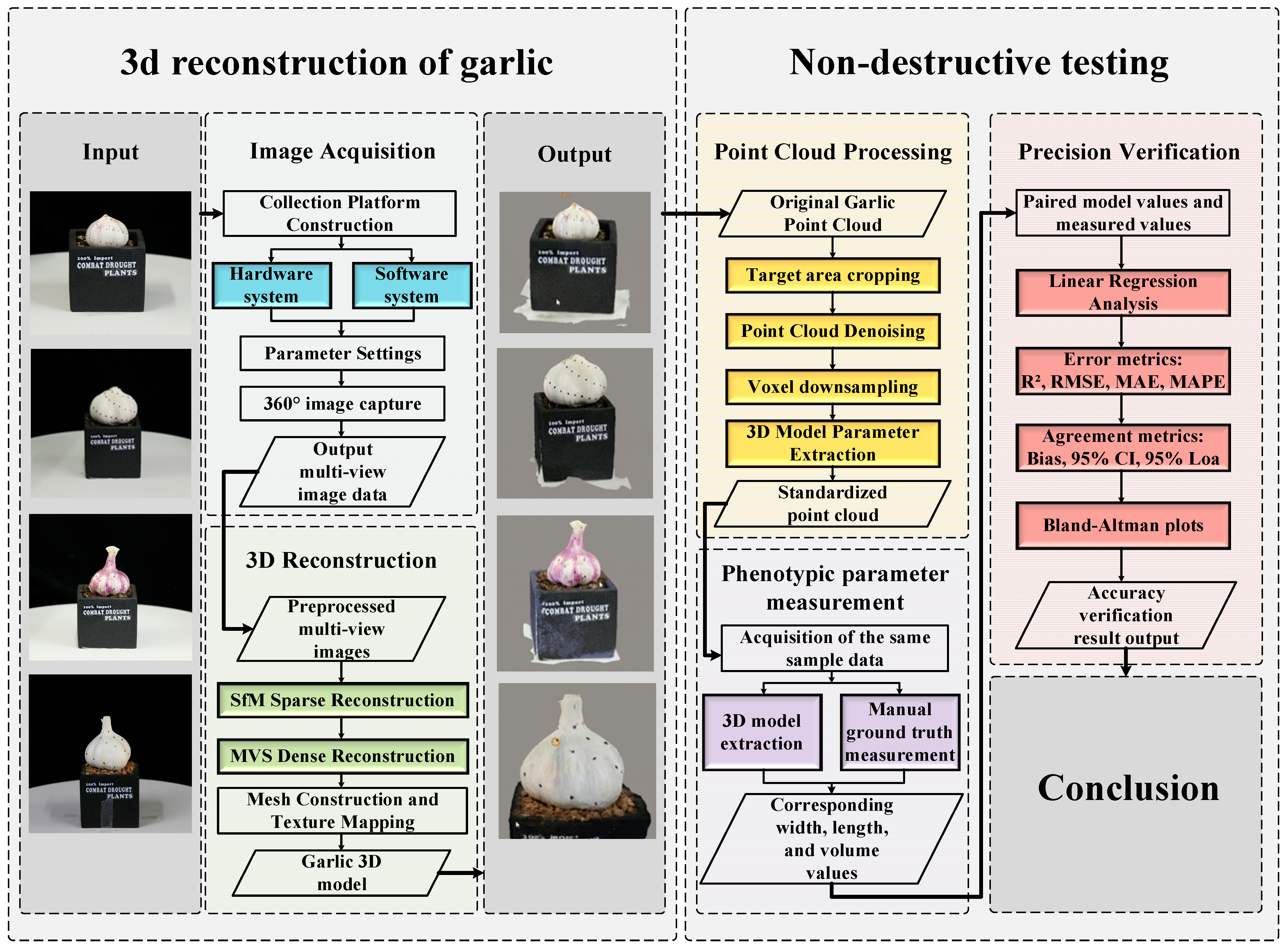
The overall technical workflow developed in this study consisted of five sequential stages: controlled multi-view image acquisition, photogrammetric three-dimensional reconstruction, point-cloud preprocessing, phenotypic parameter extraction, and accuracy validation. Multi-view images were first acquired using the standardized imaging platform and subsequently reconstructed into three-dimensional garlic bulb models. The resulting point clouds were cropped, denoised, voxel-downsampled, and pose-corrected before the maximum longitudinal diameter, maximum transverse diameter, and volume were extracted. Finally, the model-derived measurements were compared with the corresponding manual reference measurements using regression and agreement analyses. The complete workflow is illustrated in Figure 2.

2.2.2. Sample and Device Preprocessing

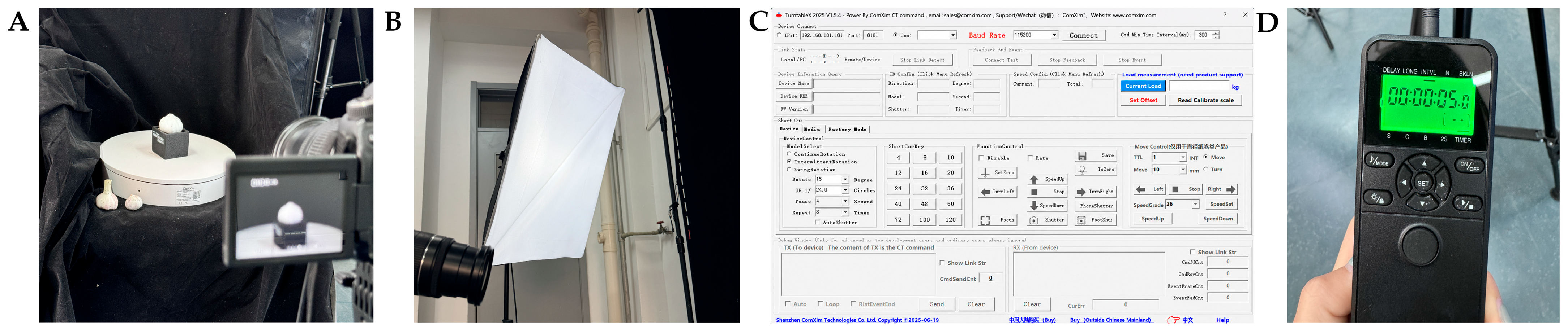
The garlic samples were removed from the constant-temperature and humidity storage chamber, rinsed with clean water to remove surface residues, and gently blotted dry with filter paper. The root end of each sample was vertically inserted into a fixation pot, with the base of the bulb kept flush with the pot rim to fully expose the measurement area. The roots were secured with substrate and gravel, and the pot was firmly attached to the motorized turntable using double-sided adhesive tape to form a stable clamping system. A low-reflection optical acquisition environment was established by constructing an enclosed background with high light-absorbing black velvet to suppress stray light and specular reflection (Figure 3A). A side-illumination setup was used to generate a uniform diffuse lighting field, reducing shadows in bulb folds and shaded regions and ensuring uniform illumination across the entire bulb surface (Figure 3B).

2.2.3. Garlic Image Data Acquisition

Multi-view image acquisition was performed using the TurntableX-controlled MT-380 motorized turntable, the Canon EOS 80D digital camera, and the Godox SL60 LED continuous light source, as shown in Figure 3. During image acquisition, each garlic bulb was fixed at the centre of the turntable, and the rotation axis was kept approximately aligned with the central axis of the bulb. The camera was mounted on a height-adjustable acquisition stand, and the optical axis of the lens was horizontally aligned with the central region of the garlic bulb to reduce perspective distortion and maintain consistent imaging geometry.

A Canon EF-S 18–135 mm lens was used, and the focal length was fixed at 50 mm throughout image acquisition. The camera-to-object distance was maintained at approximately 60 cm, allowing the complete garlic bulb and the calibration reference to be included within the image frame while maintaining sufficient image resolution for feature matching. The camera was operated in manual exposure mode. The aperture, shutter speed, and ISO were fixed at f/8, 1/60 s, and ISO 100, respectively. Manual focus was used and locked after focusing on the central region of the garlic bulb. The white balance was fixed at 5600 K to match the colour temperature of the LED light source. These fixed imaging settings were used to reduce brightness, colour, and focus variations among different viewing angles.

The Godox SL60 LED light source was positioned approximately 50 cm from the sample and arranged at an oblique angle of approximately 45° relative to the camera–sample axis, as shown in Figure 3B. A diffuser was used to soften the illumination and reduce strong shadows and specular reflections on the garlic epidermis. A matte black background was used to suppress stray light and improve the contrast between the garlic bulb and the background, as shown in Figure 3A. During the acquisition process, the relative positions of the camera, light source, background, and turntable were kept unchanged.

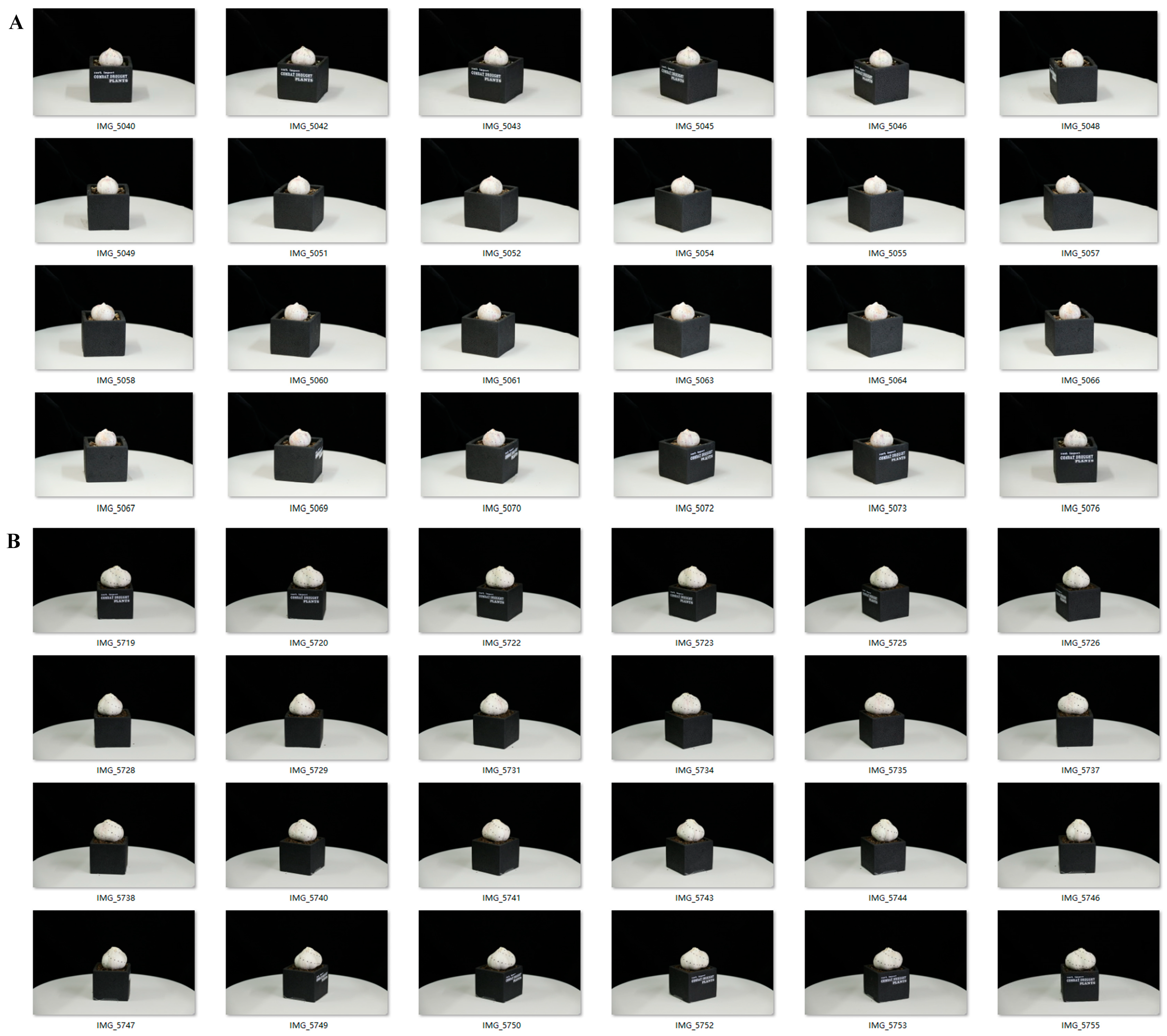
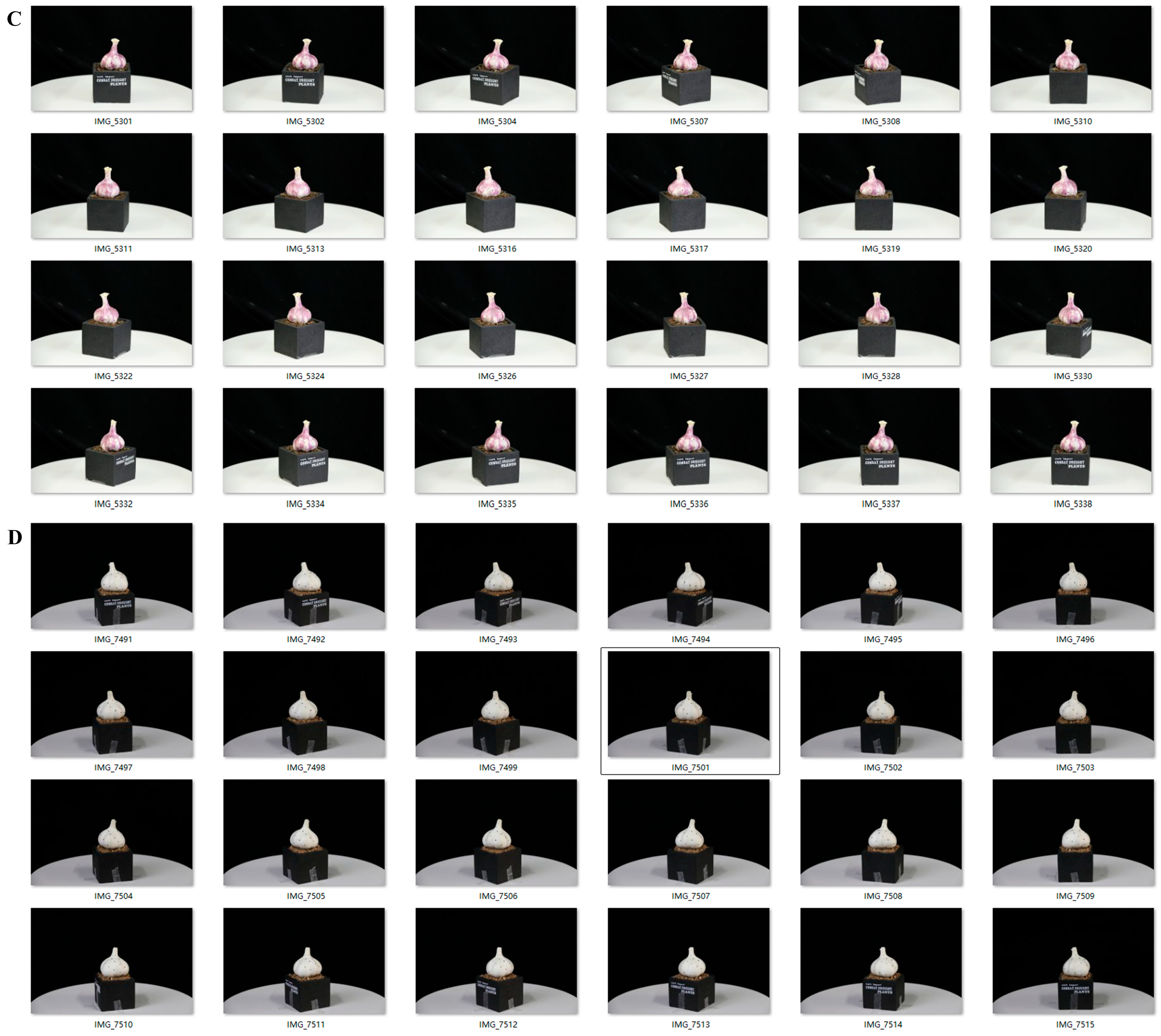
The turntable was set to a step angle of 15°, a dwell time of 4 s, and a full 360° rotation, as shown in Figure 3C. A timer-triggered shutter release was used at 5 s intervals, as shown in Figure 3D. One image was captured after the turntable had stopped at each angular position to minimize motion blur and angular deviation. Therefore, 24 images were obtained for each garlic bulb. The overlap between adjacent images was maintained at no less than two-thirds, which provided sufficient common feature points for subsequent photogrammetric reconstruction. Representative multi-view images of the garlic bulbs are shown in Figure 4.

All images were acquired in RAW format with a resolution of 6000 × 4000 pixels. Before three-dimensional reconstruction, the RAW images were converted using the same exposure, white-balance, and colour-profile settings to ensure radiometric consistency among different views. No cropping, scaling, or geometric correction was applied before reconstruction, so that the original imaging geometry could be retained for Structure-from-Motion and multi-view stereo processing.

2.2.4. Three-Dimensional Model Reconstruction of Garlic

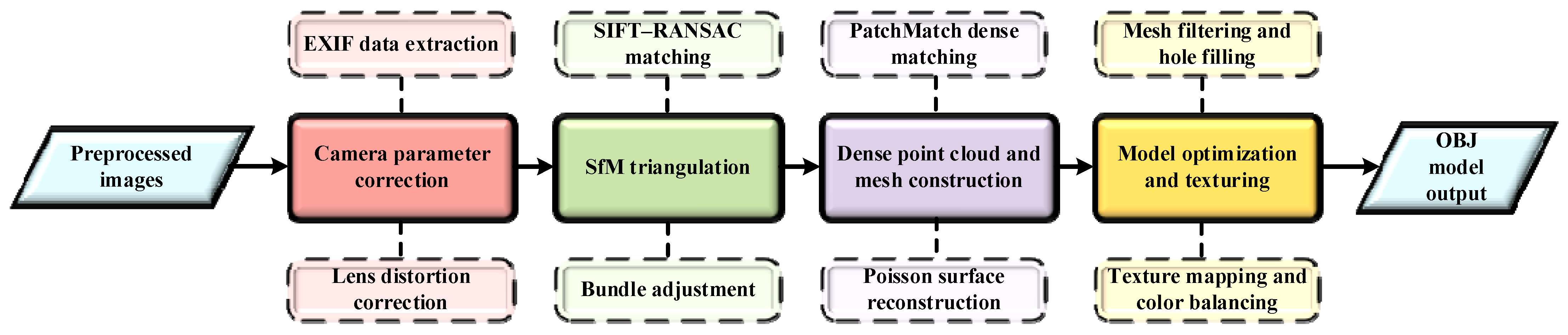
ContextCapture was used to reconstruct three-dimensional models of garlic bulbs. ContextCapture Center 64-bit, version 10.20.1.5562 is professional 3D reconstruction software based on multi-view stereo vision and photogrammetry. It can automatically estimate camera orientation from image sequences, generate dense point clouds, and reconstruct high-precision triangular mesh models, making it suitable for high-fidelity 3D digitisation of static objects. The photogrammetric reconstruction procedure implemented in ContextCapture is summarized in Figure 5.

Using the preprocessed multi-view images as input, the software first parsed the camera EXIF data to determine the initial internal orientation parameters and group the images. The camera intrinsic parameters and distortion coefficients were initialized by ContextCapture according to the EXIF information and camera model, and were further optimized automatically during aerotriangulation. No manual pre-calibrated camera parameters were imposed. A unified local coordinate system was then established, and a lens distortion model was applied to correct radial and tangential distortions, thereby providing a geometric reference for subsequent multi-view constraints. The camera distortion correction model can be expressed as follows:

$$\left\{\begin{array}{c}{x}_d=x(1+k_1{r}^2+k_2{r}^4+k_3{r}^6)+2p_{1}xy+p_2(r^2+2x^2),\\ y_d=y(1+k_1{r}^2+k_2{r}^4+k_3{r}^6)+p_1(r^2+2y^2)+2p_{2}xy,\end{array}\right.$$

(1)

where (x,y) are the normalized image coordinates before correction, $(x_d,y_d)$ are the image coordinates after applying the distortion model, $r^2=x^2+y^2$, $k_1$, $k_2$, and $k_3$ are radial distortion coefficients, and $p_1$ and $p_2$ are tangential distortion coefficients.

Cross-view correspondences are established using SIFT feature extraction [16] and RANSAC-based robust matching. The parameters for feature extraction, feature matching, and outlier rejection were kept as the default settings of ContextCapture because they are automatically controlled by the software. Aerotriangulation is then performed through bundle adjustment [17] to globally optimise the camera interior and exterior orientation parameters and the coordinates of sparse tie points. The core objective of bundle adjustment is to minimize the reprojection errors of all matched points, and its objective function can be expressed as follows:

$${arg min}_{\left\{R_i,t_i\right\},\left\{X_j\right\}}{\sum }_{i,j}\rho ({‖\pi \left(K_i\left(R_i{X}_j+t_i\right)\right)-x_{ij}‖}^2),$$

(2)

where $R_i$ and $t_i$ denote the rotation matrix and translation vector of the i-th camera, respectively; $X_j$ denotes the three-dimensional coordinate vector of the j-th point; $K_i$ denotes the camera intrinsic matrix; π(·) denotes the projection function; $x_{ij}$ denotes the observed coordinate of the j-th point in the i-th image; and ρ(·) denotes the robust loss function. Through iterative optimization, the reprojection error is controlled within 0.3 pixels, ensuring the geometric stability of the reconstruction.

Using the estimated camera poses as prior constraints, point cloud densification is performed using PatchMatch-based multi-view stereo matching to generate a high-density 3D point cloud [18]. The dense reconstruction parameters were kept as the default settings of ContextCapture. Under these settings, the point density in the garlic bulb region exceeded 500 points/mm², enabling the preservation of micro-geometric features such as epidermal folds, inter-clove boundaries, and shallow surface depressions. Subsequently, a watertight triangular mesh is generated from the dense point cloud using Poisson surface reconstruction. Poisson surface reconstruction fits the point cloud surface by solving the Poisson equation of the indicator function [19], and its core equation can be expressed as follows:

$${\nabla }^2\chi =\nabla ·V$$

(3)

where χ denotes the indicator function, and V denotes the normal vector field of the point cloud. By solving this equation and extracting the corresponding isosurface, a closed triangular mesh model was obtained. Mesh filtering and adaptive hole filling were then applied to remove non-manifold triangles, isolated components, redundant triangular faces, and local topological defects. Multi-view image textures were mapped onto the mesh surface, and illumination differences were reduced through global colour balancing, thereby generating a three-dimensional model with both geometric accuracy and realistic texture representation.

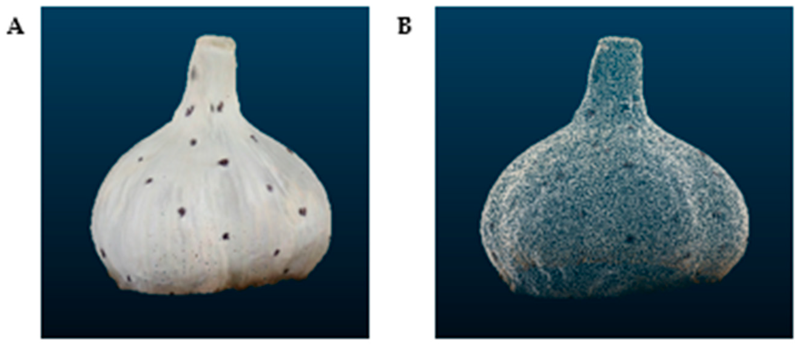
Finally, the reconstructed model was subjected to quality control in terms of completeness, mesh quality, and void areas to ensure the integrity and reliability of the model structure. The final model was exported in the universal OBJ format with a global scale factor of 1.0 (Figure 6A–D), providing a standard data container for subsequent point cloud processing, morphological parameter extraction, and accuracy verification.

2.2.5. Point Cloud Pre-Processing

The point cloud data of garlic bulbs obtained through multi-view reconstruction are large in volume and often contain outlier noise points owing to limitations in imaging equipment accuracy and interference from ambient illumination. In addition, the reconstructed point cloud models may exhibit deviations in orientation and scale relative to the actual garlic bulbs in three-dimensional space, which can impede the subsequent extraction of phenotypic parameters and accuracy evaluation. Therefore, before phenotypic feature acquisition, a series of preprocessing operations, including point cloud cropping, denoising, downsampling, and orientation correction of the model, must be performed to improve the purity, standardization, and accuracy of the point cloud data, thereby providing a reliable basis for subsequent parameter extraction.

Point Cloud Cropping

The raw point cloud of garlic bulbs obtained from multi-view three-dimensional reconstruction contains many invalid outliers, including the base of the flowerpot and the imaging background. Therefore, a combined algorithm based on RANSAC plane fitting and Z-axis pass-through filtering was used for automated point cloud cropping. This process required no manual intervention and could adaptively accommodate garlic samples with different sizes and orientations, enabling the precise removal of background outliers while fully preserving the contour of the bulb.

First, the random sample consensus (RANSAC) algorithm was used to fit the supporting plane of the flowerpot at the base, thereby removing planar noise adjacent to the bottom of the bulb. The general equation for fitting a spatial plane is expressed as follows:

$$Ax+By+Cz+D=0,$$

(4)

where A, B, and C are the coefficients of the plane normal vector and characterize the spatial orientation of the plane, and D is the plane constant term and represents the plane offset. The algorithm fits an initial plane model through random iterative sampling of local point clouds and calculates the perpendicular distance between each point and the fitted plane to distinguish in-plane points, which correspond to flowerpot noise, from out-of-plane points, which correspond to valid bulb points. The distance from a point to a plane is calculated as follows:

$$d_i={\displaystyle \frac{\left|A{x}_i+B{y}_i+C{z}_i+D\right|}{\sqrt{A^2+B^2+C^2}}},$$

(5)

where $d_i$ denotes the perpendicular distance from the i-th point to the fitted plane, and ($x_i,y_i,z_i$) denotes the three-dimensional coordinates of the corresponding point.

In this study, RANSAC plane fitting was used to identify and remove the supporting plane and flowerpot-related background points. The distance threshold $d_0$ was set to 0.20 cm, the maximum number of iterations was set to 1000, and the confidence level was set to 0.99. During iterative plane fitting, points with a perpendicular distance less than or equal to $d_0$ were classified as inliers of the supporting plane. These points were identified as background noise originating from the flowerpot or substrate and were therefore removed. Points with a distance greater than ${\mathrm{d}}_0$ were retained as candidate garlic bulb point-cloud data. By repeatedly sampling the minimum point set and updating the plane parameters, the plane model with the largest number of inliers was selected as the optimal fitted plane [20]. This procedure reduced the influence of scattered outliers on plane estimation and enabled the removal of planar noise adjacent to the bulb base.

After planar outliers were removed, a Z-axis pass-through filtering algorithm was applied for a second stage of refined denoising [21]. Because the longitudinal axis of each garlic bulb was aligned with the spatial Z-axis, vertical coordinate screening criteria were established according to the height distribution characteristics of the samples. The filtering decision criterion was defined as follows:

$$S=\left\{P_i(x_i,y_i,z_i)|z_{low}\le z_i\le z_{high}\right\}$$

(6)

where S denotes the valid bulb point cloud set after cropping, $z_{\mathit{low}}$ denotes the critical height threshold at the bottom of the bulb, and $z_{\mathit{high}}$ denotes the maximum height threshold at the top of the bulb. In this study, $z_{\mathit{low}}$ was set to 0.10 cm above the fitted support plane to remove residual flowerpot, substrate, and low-elevation noise points near the basal region. The upper threshold $z_{\mathit{high}}$ was set to 8.00 cm above the fitted support plane to retain the complete bulb region while removing isolated high-elevation background points. This threshold range covered the measured longitudinal diameter range of the validation samples and avoided excessive removal of valid bulb points.

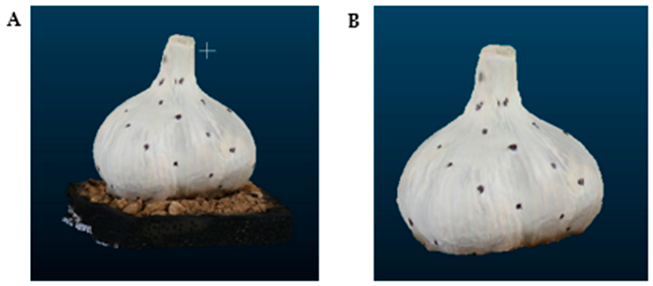
Through the combination of RANSAC plane fitting and Z-axis pass-through filtering, background interference points around the supporting plane and residual outliers outside the bulb height range were effectively removed. Compared with cropping using a single fixed boundary, this combined strategy reduced the risk of over-cropping or under-cropping near the bulb base and better preserved the basal contour, edge details, and three-dimensional geometric structure of the garlic bulb. The cropped point cloud provided a cleaner and more reliable input for subsequent denoising, downsampling, pose correction, and phenotypic parameter extraction, as shown in Figure 7A,B.

Point Cloud Denoising

During 3D reconstruction, factors such as equipment precision, ambient lighting variations, and camera shake can introduce numerous outliers and noise points into the point cloud data. These noise points may cause errors in subsequent phenotypic parameter extraction, increase computational burden, and reduce processing efficiency. Therefore, the statistical outlier removal (SOR) filtering algorithm was applied to remove isolated noise points from the reconstructed garlic bulb point clouds [22].

In this study, SOR filtering was performed in CloudCompare. The number of nearest neighbours, k, was set to 30, and the standard deviation multiplier, λ was set to 1. For each point, the average distance $d_i$ to its 30 nearest neighbouring points was first calculated. The mean value μ and standard deviation σ of all average neighbour distances were then computed. A maximum distance threshold $D_{max}$ was defined as follows:

$$\sigma =\sqrt{{\displaystyle \frac{{\sum }_{i=1}^n{(d_i-\mu )}^2}{n}},}$$

(7)

$$D_{max}=\mu +\lambda \times \sigma .$$

(8)

Points with an average neighbour distance greater than $D_{max}$ were identified as outliers and removed. The value k = 30 was selected to balance noise removal and local geometric detail preservation. A smaller neighbourhood may be more sensitive to isolated points, whereas an excessively large neighbourhood may smooth local features and remove valid points around clove boundaries, epidermal folds, and the basal contour of garlic bulbs. Therefore, the combination of k = 30 and λ = 1 was applied consistently to all garlic bulb point clouds before downsampling and phenotypic parameter extraction.

Point Cloud Downsampling

The dense point cloud of garlic bulbs generated by multi-view reconstruction contains a large number of data points, which substantially increases the computational burden of subsequent point cloud processing and phenotypic parameter extraction. Moreover, redundant points did not necessarily improve the accuracy of parameter extraction. Therefore, voxel grid downsampling was applied to simplify the dense point cloud while preserving the main geometric structure of the garlic bulb [23].

In this study, voxel grid downsampling was performed in CloudCompare using a voxel size of 0.5 mm. The voxel size was determined based on a preliminary comparison among three voxel sizes, namely 0.1 mm, 0.2 mm, and 0.5 mm, with the aim of balancing point-cloud simplification and geometric-detail preservation. When the voxel size was set to 0.1 mm, the local surface details of the garlic bulb were well preserved; however, the reduction in point number was limited, and the improvement in computational efficiency was not obvious. When the voxel size was set to 0.2 mm, the point cloud was simplified to a certain extent, but a large number of redundant points still remained. In contrast, a voxel size of 0.5 mm effectively reduced redundant points and improved processing efficiency while preserving the main contour, shallow depressions, epidermal folds, and inter-clove boundary features of the garlic bulb. Moreover, compared with the original dense point cloud, the differences in the extracted maximum longitudinal diameter, maximum transverse diameter, and volume were within the acceptable measurement tolerance under the 0.5 mm setting. Therefore, 0.5 mm was selected as the final voxel size and was applied consistently to all garlic bulb point clouds before pose correction and phenotypic parameter extraction.

The three-dimensional point-cloud space was divided into cubic voxels with an edge length of 0.5 mm. For each voxel, the centroid of all points within the voxel was calculated, and all original points in that voxel were replaced by a single representative centroid point. The formula for calculating the voxel center of mass is as follows:

$$P_c(x_c,y_c,z_c)=({\displaystyle \frac{1}{N_v}}{\displaystyle {\sum }_{i=1}^{N_v}}{x}_i,{\displaystyle \frac{1}{N_v}}{\displaystyle {\sum }_{i=1}^{N_v}}{y}_i,{\displaystyle \frac{1}{N_v}}{\displaystyle {\sum }_{i=1}^{N_v}}{z}_i),$$

(9)

where $P_c$ denotes the centroid point representing a single voxel, $N_v$ denotes the number of original point cloud points contained in the voxel, and $x_i,y_i,\mathrm{a}\mathrm{n}\mathrm{d} z_i$ denote the three-dimensional coordinates of the i-th original point cloud point within the voxel, respectively.

The voxel size of 0.5 mm was selected to balance point-cloud simplification and geometric detail preservation. A larger voxel size could further reduce the number of points and improve processing efficiency, but it may weaken local contour features, especially around clove boundaries, epidermal folds and the basal edge of garlic bulbs. In contrast, a smaller voxel size would retain more surface details but increase computational cost and provide limited additional benefit for extracting centimetre-scale phenotypic parameters. Therefore, a voxel size of 0.5 mm was applied consistently to all garlic bulb point clouds before pose correction and phenotypic parameter extraction.

Compared with random downsampling, voxel grid downsampling achieved more uniform point-cloud reduction through spatially regular grid sampling. This method removed redundant point-cloud data while preserving the three-dimensional morphology, edge contours and fine surface structural features of garlic bulbs. Consequently, it reduced the computational cost of subsequent phenotypic parameter estimation while maintaining the geometric integrity required for accurate extraction of maximum transverse diameter, maximum longitudinal diameter and volume. The effect of voxel grid downsampling is shown in Figure 8A,B.

Point Cloud Pose Correction

Due to variations in shooting angles during the reconstruction process, the generated point cloud models of garlic bulbs are prone to spatial pose deviations. These deviations cause a mismatch between the spatial coordinate system of the point cloud and the natural growth posture of the garlic bulb, which directly affects the accurate calculation of geometric parameters, such as length, width, and volume, and consequently leads to errors in phenotypic measurement. Therefore, principal component analysis (PCA) was employed to align the bulb point cloud by correcting the principal longitudinal axis of the bulb to coincide with the spatial Z-axis [24].

The total number of points in the garlic bulb point cloud was denoted as N, and the three-dimensional coordinates of the i-th point were denoted as $P_i(x_i,y_i,z_i)$. The overall centroid coordinate of the point cloud, $\overline{P}(\overline{x},\overline{y},\overline{z})$, was calculated as follows:

$$\overline{x}={\displaystyle \frac{1}{N}}{\sum }_{i=1}^N{x}_i, \overline{y}={\displaystyle \frac{1}{N}}{\sum }_{i=1}^N{y}_i, \overline{z}={\displaystyle \frac{1}{N}}{\sum }_{i=1}^N{z}_i,$$

(10)

the point cloud was then centered by subtracting the centroid coordinate from each point, and the three-dimensional covariance matrix C was constructed as follows:

$$C={\displaystyle \frac{1}{N}}{\sum }_{i=1}^N(P_i-\overline{P}){(P_i-\overline{P})}^T,$$

(11)

eigenvalue decomposition was then performed on the covariance matrix as follows:

$$C{v}_j={\lambda }_j{v}_j,$$

(12)

where ${\lambda }_j$ denotes the eigenvalue, and $v_j$ denotes the corresponding eigenvector. The eigenvalues were sorted in descending order as ${\lambda }_1{>\lambda }_2{>\lambda }_3$. The eigenvector $v_1$ corresponding to the largest eigenvalue represents the principal direction of spatial extension of the garlic bulb and was therefore defined as the longitudinal axis of the bulb.

A spatial rotation matrix R was constructed using the principal eigenvector as a reference, and a rotation transformation was applied to the point cloud coordinates for orientation correction as follows:

$${P_i}^{\prime }=R(P_i-\overline{P}),$$

(13)

where ${P_i}^{\prime }$ denotes the three-dimensional coordinate of the orientation-corrected point cloud.

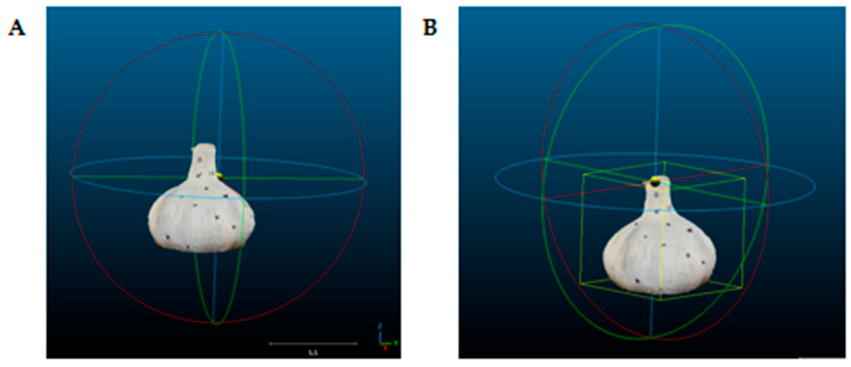
After the PCA-based rotation transformation, the overall longitudinal axis of the garlic bulb was aligned with the Z-axis in three-dimensional space (Figure 9A,B). In this study, PCA-based pose correction was performed after point-cloud cropping, denoising and voxel downsampling. The eigenvector corresponding to the largest eigenvalue was defined as the principal longitudinal direction of the garlic bulb and was rotated to align with the spatial Z-axis. To ensure consistency among samples, the same pose-correction procedure was applied to all garlic bulb point clouds before extracting the maximum transverse diameter, maximum longitudinal diameter and volume. No manual adjustment of the bulb orientation was performed after PCA correction. All samples were unified into a standard spatial orientation, thereby eliminating spatial pose discrepancies caused by shooting angles and placement inclination. This process provided a normalized geometric reference for the accurate quantitative extraction of longitudinal diameter, transverse diameter, and volume in subsequent analyses.

After the aforementioned preprocessing steps, redundant and noisy points were effectively removed from the garlic bulb point cloud. The resulting point cloud had an appropriate density and standardized spatial orientation, accurately represented the actual morphology of the garlic bulbs, and could be directly used for subsequent phenotypic parameter extraction and accuracy validation.

2.2.6. Extraction of Garlic Model Phenotypic Parameters

According to the requirements of the Chinese national standard GB/T 45244-2025 [15], Garlic Grade Specification, the core phenotypic parameters extracted in this study were determined as the maximum transverse diameter, maximum longitudinal diameter, and volume of the garlic bulb.

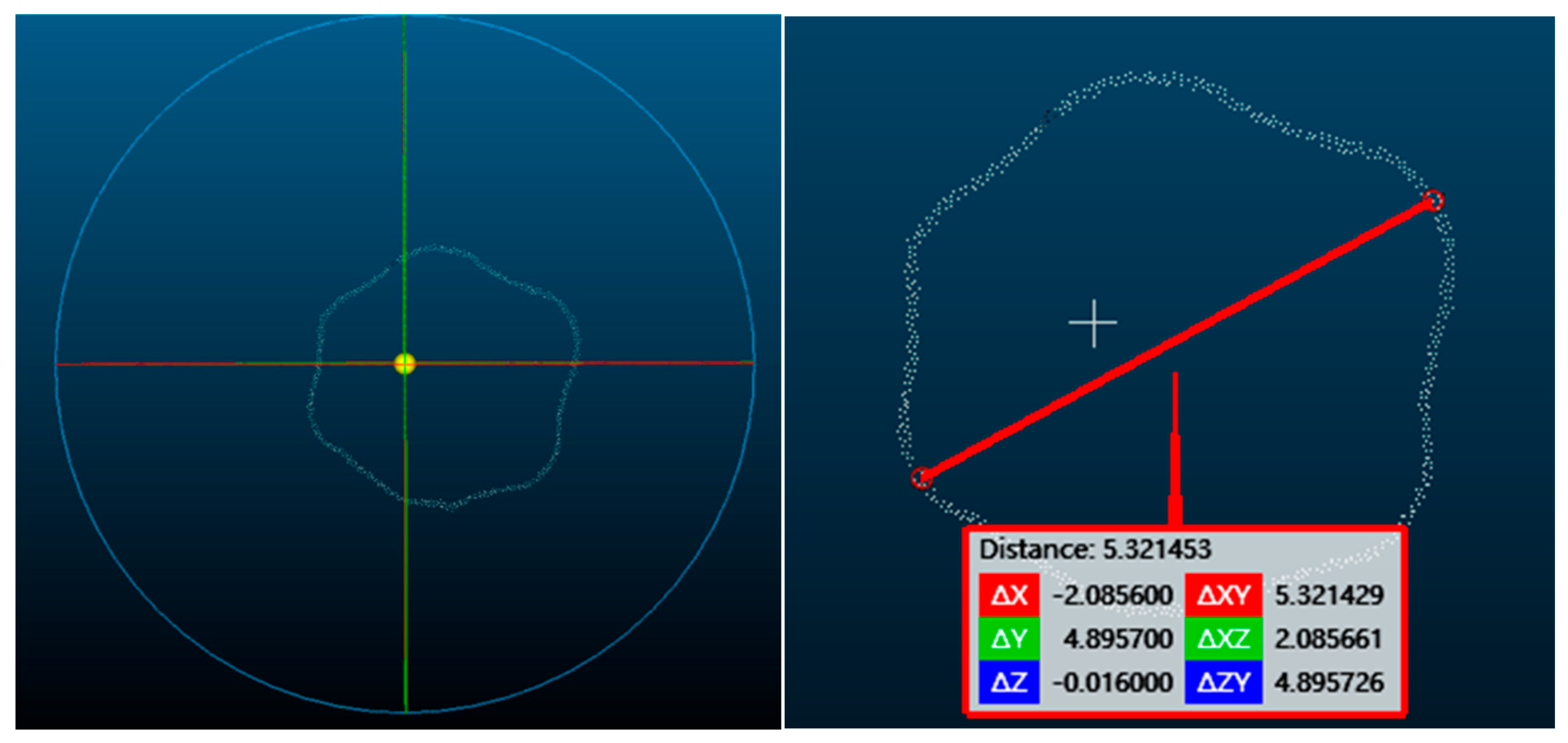
In the CloudCompare environment, the maximum transverse diameter of the garlic bulb was extracted based on the true scale and spatial geometric features of the model. After the three-dimensional model was imported, the bounding box analysis function in the software was used to obtain the geometric distribution characteristics of the bulb in the XY plane. Using the geometric center of the model as the reference point, the extreme contour points in different directions within the horizontal plane were identified. The Euclidean distances between opposing contour points were then calculated, and the maximum distance was defined as the maximum transverse diameter of the sample (Figure 10) [25]. Under the real-scale constraint with a global model scale factor of 1.0, the extracted distance directly represented the actual maximum transverse dimension in physical space, thereby providing objective and reproducible measurement results.

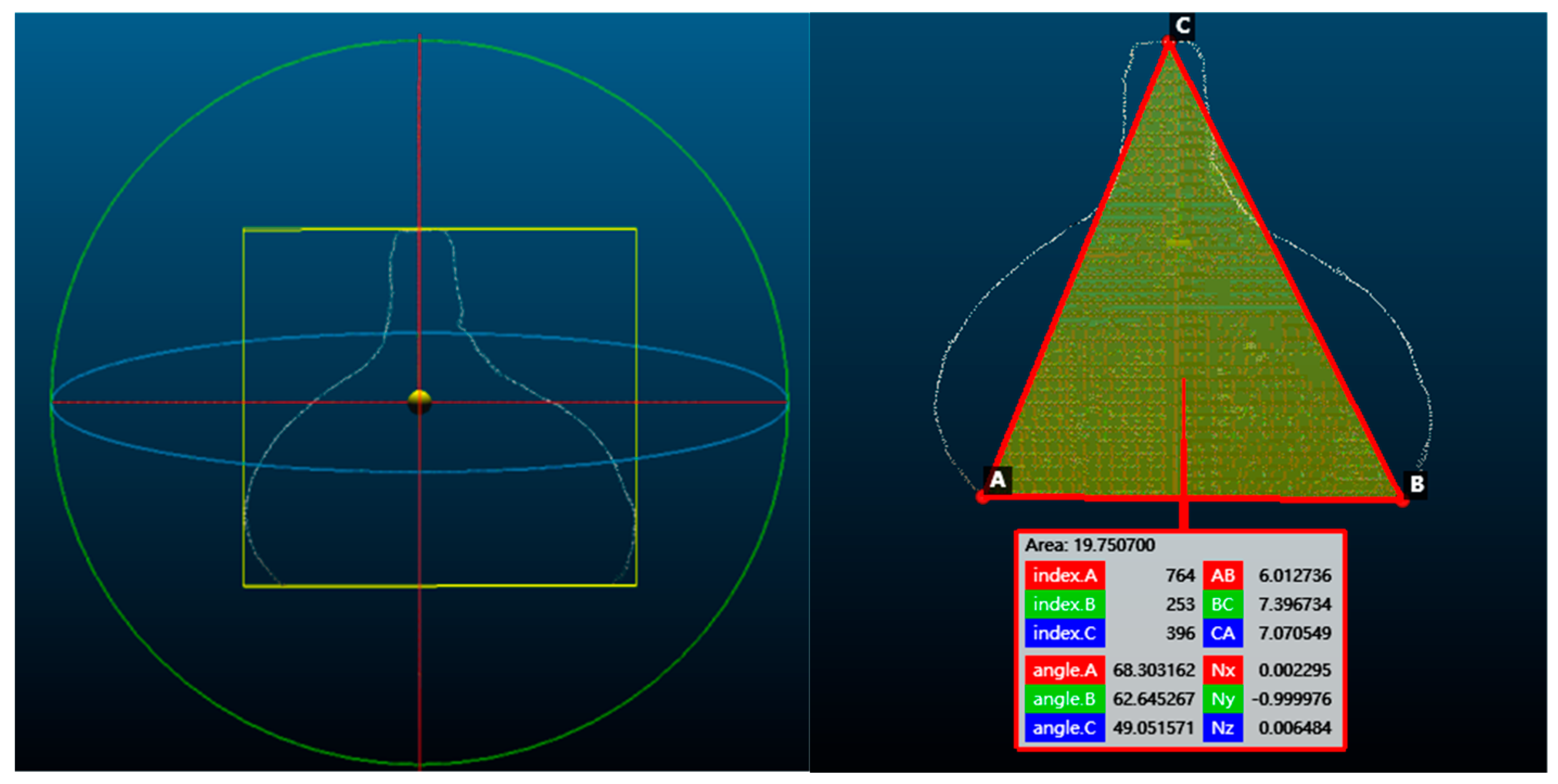
The longitudinal diameter of garlic bulbs was extracted using a method based on geometric constraints of the longitudinal cross-sectional contour, thereby reducing the effect of missing basal point cloud data on the direct extremum method. Because the base of the garlic bulb was connected to the growing medium, the point cloud at the contact region between the bulb base and the medium was also removed during background point cloud removal. Consequently, the bottom of the bulb point cloud formed a natural “open boundary”, preventing the complete longitudinal diameter from being obtained directly from the difference between the extreme values in the Z direction. Therefore, a triangular height calculation method based on a three-point contour constraint was used for longitudinal diameter estimation.

First, a longitudinal slice was obtained along the growth axis of the bulb to extract the cross-sectional contour. The two outermost endpoints of the bottom contour in this cross-section were defined as A and B, while the highest point of the upper bulb contour was defined as C, thereby constructing the spatial triangle △ABC. In this triangle, line segment AB represented the effective width of the basal cross-section of the bulb, whereas line segments AC and BC represented the contour edges connecting the basal endpoints to the apex.

Based on the geometric relationships of a triangle, the longitudinal diameter H of the bulb was defined as the length of the perpendicular line drawn from vertex C to the base AB. This value was derived using Heron’s formula as follows:

$$s={\displaystyle \frac{L_{AB}+L_{AC}+L_{BC}}{2}},$$

(14)

$$H={\displaystyle \frac{2\sqrt{s(s-L_{AB})(s-L_{AC})(s-L_{BC})}}{L_{AB}}},$$

(15)

where $L_{AB}$ denotes the distance between the two bottom points, $L_{AC} \mathrm{a}\mathrm{n}\mathrm{d} L_{BC}$ denote the contour distances from the two bottom endpoints to the top vertex, respectively, and s denotes the semi-perimeter of the triangle. This method uses contour-based geometric constraints to achieve stable estimation of the longitudinal diameter even when the point cloud at the base is incomplete, thereby avoiding underestimation of the extreme value caused by missing bottom points.

Simultaneously, the orthogonality between the cross-section and the growth axis was verified using the plane normal vector of the triangle, (N_x,N_y,N_z). This ensured that the direction of the perpendicular line was aligned with the actual growth axis of the bulb and eliminated systematic errors caused by slice inclination. Under the true-scale constraint provided by a unit global scaling factor of 1.0, the calculated length of the perpendicular line directly represented the actual maximum longitudinal diameter of the bulb, as illustrated in Figure 11.

Bulb volume was quantitatively extracted using the rasterized projection integration method [26]. This method uses the spatial distribution characteristics of the point cloud to convert three-dimensional volume calculation into the summation of two-dimensional raster areas. The point cloud space was divided into a series of equally spaced projection planes along the growth axis of the bulb, and the point cloud within each plane was rasterized to generate a two-dimensional projection raster map. Subsequently, the average height of the point cloud within each grid cell was calculated, and the product of the grid area and height was used as the volume contribution of that cell. Finally, the total bulb volume was obtained by summing the volume contributions of all grid cells. The calculation formula is as follows:

$$V={\sum }_{i=1}^m{\sum }_{j=1}^n{S}_{ij}{h}_{ij},$$

(16)

where V denotes the total volume of the bulb, $S_{\mathit{ij}}$ denotes the area of the grid cell in the i-th row and j-th column, $h_{ij}$ denotes the average height of the point cloud within this grid cell, and m and n denote the number of rows and columns in the raster image, respectively.

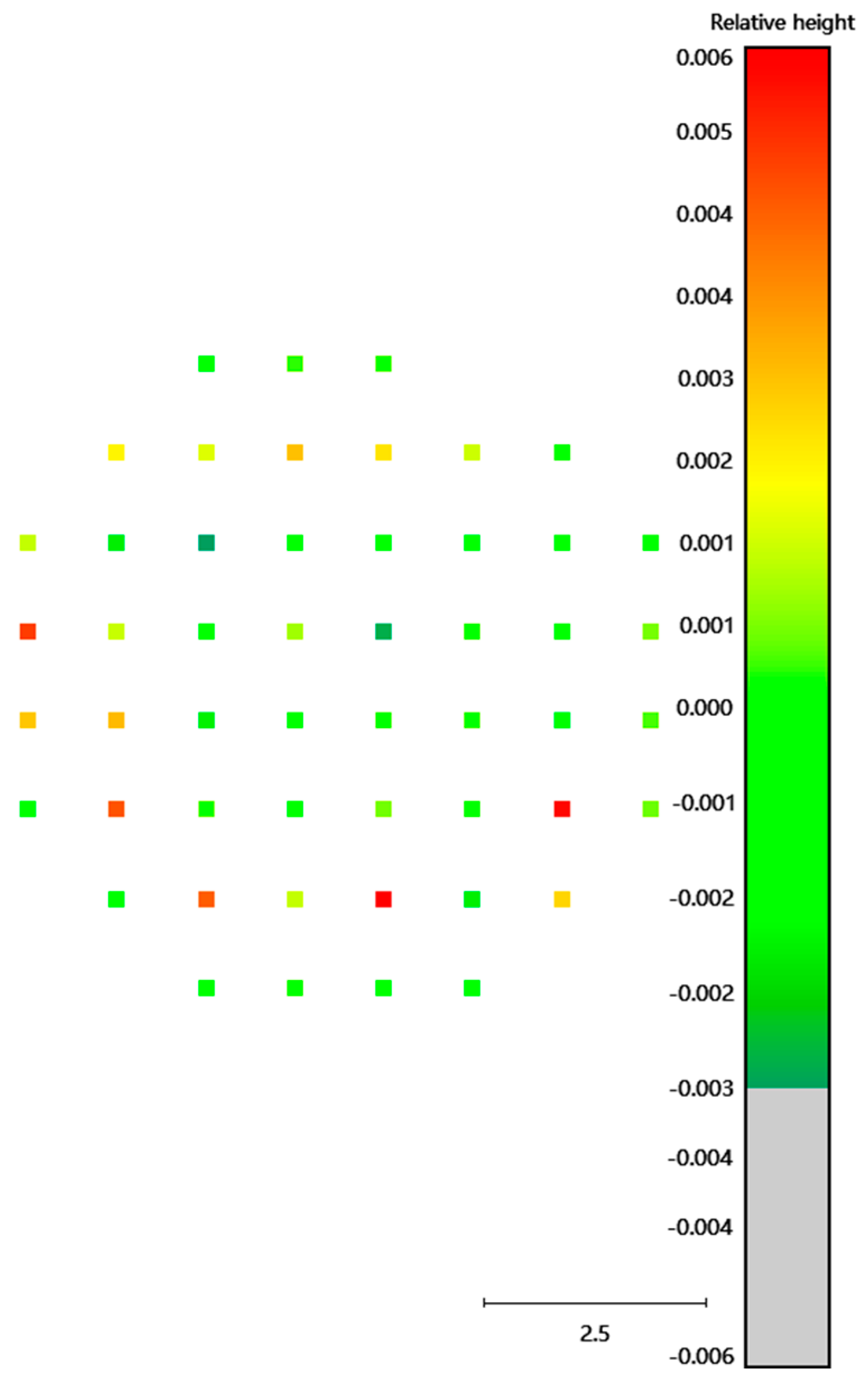
When the garlic bulb point cloud was analyzed using the raster-based volume calculation method, the relative height distribution map along the Z-axis showed that most of the main bulb region appeared dark green, with height deviations concentrated at extremely low levels close to zero (Figure 12). This result indicates a high degree of consistency between the three-dimensional model and the actual morphology of the garlic bulb. The scattered red and yellow outliers in the figure were mainly distributed in the basal region of the bulbs. This phenomenon was primarily caused by boundary effects associated with bottom clipping during the preprocessing stage and represents a normal error in the data processing procedure. Statistical analysis showed that the overall grid matching rate reached 100%, indicating the high geometric accuracy and robustness of the three-dimensional reconstruction model developed in this study. These results demonstrate that the model can meet the requirements for high-precision extraction of garlic phenotypic parameters.

2.2.7. Obtaining Ground Truth

To quantitatively evaluate the reliability of the phenotypic parameter extraction method, manual reference measurements were used as the ground truth and compared with the values extracted from the 3D model. Garlic bulb samples corresponding to those used for 3D reconstruction were selected for the experiment. The maximum transverse diameter, maximum longitudinal diameter, and volume of each sample were manually measured to obtain standard reference values corresponding one-to-one with the parameters extracted from the model, thereby providing a unified benchmark for subsequent accuracy validation.

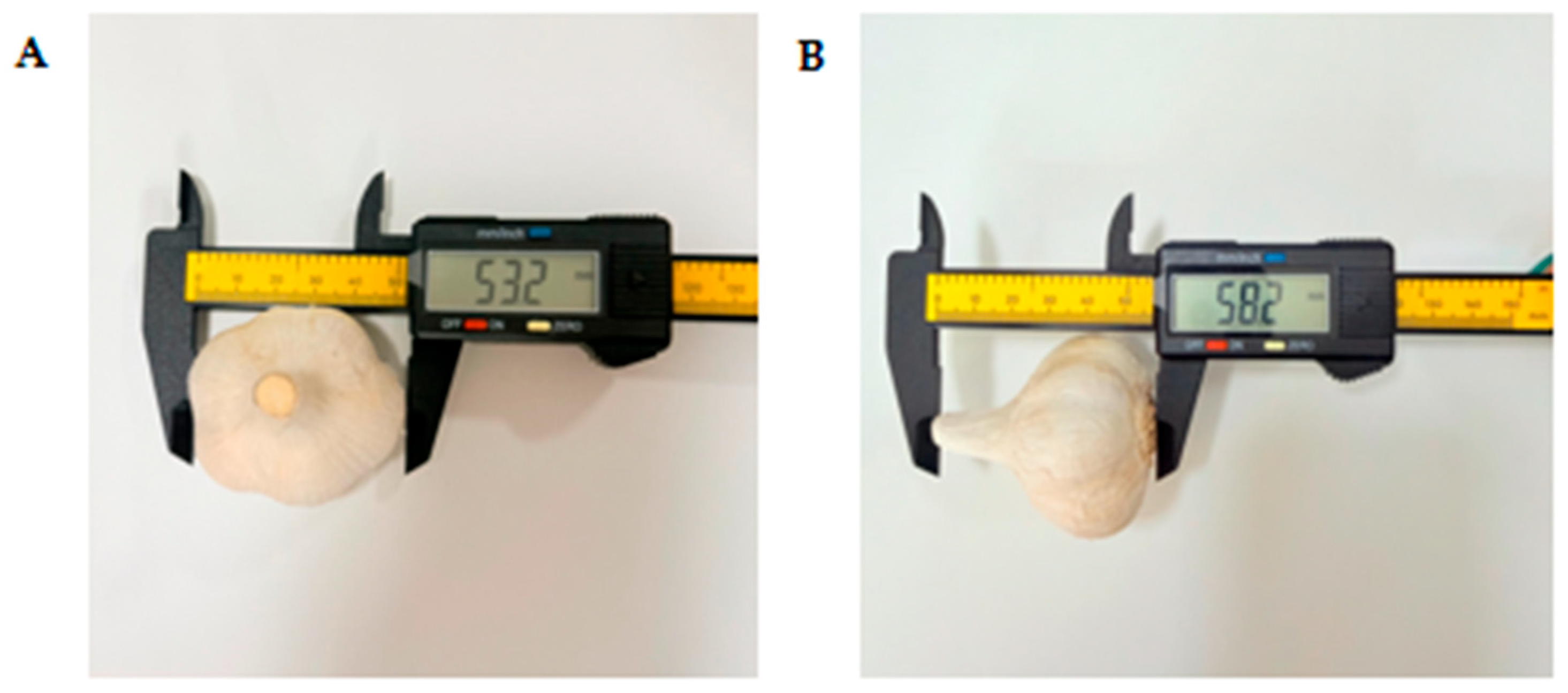
The maximum transverse diameter and maximum longitudinal diameter were measured using a digital vernier caliper with a resolution of 0.01 mm. The caliper was zero-calibrated before measurement to reduce systematic error. All diameter measurements were performed by the same trained operator under the same measurement procedure. For transverse diameter measurement, the widest equatorial region of each bulb was selected, as shown in Figure 13A, and three representative directions around the bulb circumference were measured. Each direction was measured twice, and the mean value of all repeated measurements was used as the manual reference value. For longitudinal diameter measurement, each bulb was placed on a horizontal surface and adjusted so that the apical and basal ends were aligned in the same vertical plane, as shown in Figure 13B. The maximum straight-line distance from the most prominent apical point to the basal end was measured three times, and the mean value was used as the manual reference value.

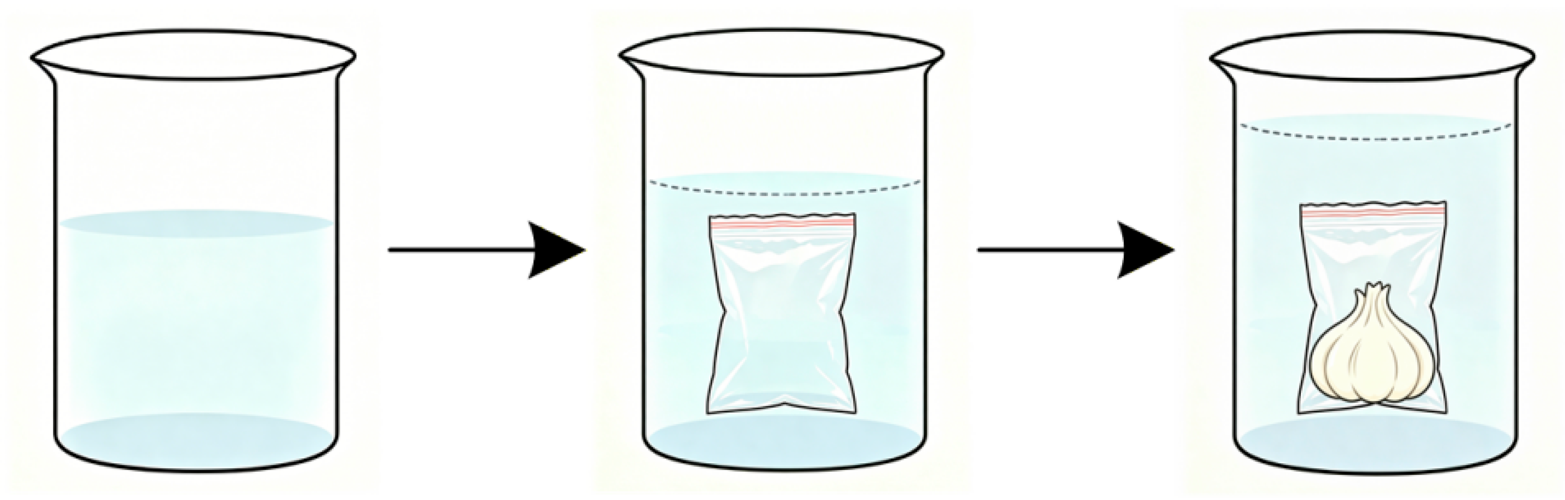
Bulb volume was measured using a modified high-precision displacement method (Figure 14). To prevent water absorption by the garlic bulbs and reduce the influence of surface wetting on measurement accuracy, each bulb was wrapped with food-grade elastic film and vacuum-sealed before immersion. This step allowed the film to adhere tightly to the bulb surface without gaps, air bubbles, or creases, thereby reducing measurement errors caused by trapped air or incomplete surface contact [27,28]. The volume of the empty wrapping material was measured separately and subtracted from the total displacement volume of the wrapped bulb. Each bulb volume was measured in triplicate, and the mean value was used as the manual reference volume.

First, the volume $V_b$ of the empty vacuum bag was measured. After the air was evacuated from the bag, it was immersed in the container, and the rise in liquid level, $h_1$, was recorded. The volume of the bag was calculated using the base area S of the container as follows:

$$V_b=S·h_1$$

(17)

Next, the total volume $V_{total}$ of the film-wrapped garlic bulb was measured. The air was evacuated again from the film-wrapped garlic bulb, after which it was immersed in water, and the rise in water level, $h_2$, was recorded. The total volume was then calculated as follows:

$$V_{total}=S·h_2$$

(18)

Finally, the volume of the wrapping material was subtracted to obtain the true volume of the garlic bulb:

$$V_{true}=V_{total}-V_b$$

(19)

All volume measurements were performed in triplicate, and the mean value was used to improve the reliability of the results.

To further verify the reliability of the modified displacement method, three rigid steel spheres with known volumes of 25, 40, and 55 cm³ were measured using the same wrapping, vacuum-sealing, immersion, and wrapping-material correction procedure. Each steel sphere was measured five times. The absolute error, relative error, and coefficient of variation were calculated to evaluate the uncertainty introduced by film wrapping, residual trapped air, vacuum sealing, and water-level reading.

Each steel sphere was measured using the same modified displacement procedure as that used for garlic bulbs. Briefly, the sphere was wrapped with food-grade elastic film, vacuum-sealed, visually inspected to ensure that no visible trapped air, wrinkles, or incomplete sealing were present, and then fully immersed in water. The volume of the empty wrapping material was measured separately and subtracted from the total displacement volume of the wrapped object. To reduce random measurement error, each steel sphere was measured five times, and the mean value was used as the displacement-derived volume.

The absolute error, relative error, and coefficient of variation were calculated to evaluate the uncertainty introduced by film wrapping, residual trapped air, vacuum sealing, and water-level reading. The absolute error and relative error were calculated as follows:

$$AE=|V_{measured}-V_{ref}|,$$

(20)

$$RE={\displaystyle \frac{|V_{measured}-V_{ref}|}{V_{ref}}}\times 100\%,$$

(21)

where $V_{ref}$ is the known reference volume of the steel sphere, and $V_{measured}$ is the volume obtained using the modified displacement method. The coefficient of variation was calculated from repeated measurements to evaluate the repeatability of the displacement procedure.

2.2.8. Accuracy Evaluation and Statistical Analysis

To quantitatively evaluate the accuracy of phenotypic measurements extracted from three-dimensional models of garlic bulbs based on multi-view reconstruction, manual measurements were used as the ground truth. Accuracy validation was performed for longitudinal diameter, transverse diameter, and volume. The coefficient of determination (R²), root mean square error (RMSE), mean absolute error (MAE), mean absolute percentage error (MAPE), and bias were adopted as comprehensive evaluation metrics to characterize the correlation, absolute error, relative error, and systematic deviation between the model-extracted results and the manually measured ground truth [29]. Because R² mainly reflects the strength of linear association and does not alone demonstrate agreement between two measurement methods, Bland–Altman analysis was further introduced to evaluate measurement agreement and the 95% limits of agreement. Linear regression scatter plots were used to visualize the correlation and fitting characteristics, whereas Bland–Altman plots were used to visualize the difference distribution, mean bias, and agreement limits between manual and model-derived measurements.

The coefficient of determination, R², was used to characterize the linear fit between the model-derived measurements and the manual reference measurements, thereby quantifying the correlation and consistency between the two datasets. Its value ranges from 0 to 1. A value closer to 1 indicates a stronger correlation between the model measurements and the true values, as well as higher fitting accuracy [30]. The calculation formula is expressed as follows:

$$R^2=1-{\displaystyle \frac{{\sum }_{i=1}^n{\left(y_i-\widehat{y_i}\right)}^2}{{\sum }_{i=1}^n{\left(y_i-\overline{y}\right)}^2}},$$

(22)

where $y_i$ denotes the manually measured ground truth, ${\hat{\mathrm{y}}}_{\mathrm{i}}$ denotes the model-extracted value, n denotes the sample size, and $\overline{y}$ denotes the arithmetic mean of the manual reference measurements.

Root mean square error (RMSE) was used to characterize the overall error level between the model measurements and the manual reference measurements. Its unit is consistent with that of the original measurement metric, and it provides an intuitive reflection of the magnitude of absolute deviation and the degree of dispersion in the model measurement results [31]. A smaller RMSE value indicates a smaller deviation between the model-extracted results and the actual measured values, reflecting higher measurement stability and accuracy of the algorithm [32]. The calculation formula is expressed as follows:

$$RMSE=\sqrt{{\displaystyle \frac{1}{n}}{\sum }_{i=1}^n{\left(y_i-\widehat{y_i}\right)}^2}$$

(23)

Mean absolute error (MAE) was used to quantify the average absolute deviation between the two measurement methods. Compared with RMSE, MAE is less affected by individual large errors and provides a direct measure of average measurement deviation. It is calculated as follows:

$$MAE={\displaystyle \frac{1}{n}}{\sum }_{i=1}^n\left|y_i-\widehat{y_i}\right|$$

(24)

Mean absolute percentage error (MAPE) was used to quantify the average relative deviation between the model-measured values and the manually measured true values as a percentage. This metric reduces, to a certain extent, the influence of differences in units and numerical scales among different phenotypic parameters on error assessment. Therefore, it is suitable for standardized comparison of measurement accuracy across different phenotypic parameters, such as transverse diameter, longitudinal diameter, and volume [33]. A lower MAPE value indicates a smaller relative deviation between the model-extracted results and the true measured values, suggesting higher measurement accuracy of the algorithm. It is calculated as follows:

$$MAPE={\displaystyle \frac{100\%}{n}}{\sum }_{i=1}^n\left|{\displaystyle \frac{y_i-\widehat{y_i}}{y_i}}\right|$$

(25)

Bias was calculated as the mean difference between the model-derived values and the manual reference measurements. It was used to determine whether the proposed method produced systematic overestimation or underestimation. The bias was calculated as follows:

$$Bias={\displaystyle \frac{1}{n}}{\displaystyle {\sum }_{i=1}^n}\left(\widehat{y_i}-y_i\right)$$

(26)

In Bland–Altman analysis, the difference between the model-derived value and the manually measured value was calculated for each sample as follows:

$$d_i=\widehat{y_i}-y_i$$

(27)

The standard deviation of the differences was calculated as follows:

$$S{D}_d=\sqrt{{\displaystyle \frac{{\displaystyle {\sum }_{i=1}^n}{\left(d_i-\overline{d}\right)}^2}{n-1}}},$$

(28)

where $d_i$ denotes the difference between the two measurement methods for the i-th sample, $\overline{d}$ denotes the mean difference, and $S{D}_d$ denotes the standard deviation of the differences. The 95% confidence interval of the bias was calculated to evaluate the uncertainty of the systematic difference between the two measurement methods:

$$C{I}_{bias}=Bias\pm t_{0.975,n-1}\times {\displaystyle \frac{S{D}_d}{\sqrt{n}}},$$

(29)

where $C{I}_{bias}$ denotes the 95% confidence interval of the bias, and $t_{0.975,n-1}$ denotes the critical value of the t-distribution with n − 1 degrees of freedom. The 95% limits of agreement were calculated as follows:

$$LoA=Bias\pm 1.96\times S{D}_d,$$

(30)

where LoA denotes the 95% limits of agreement. The upper and lower limits of agreement were used to evaluate the range within which most differences between manual and model-derived measurements were expected to fall.

Visualization of the multi-indicator regression analysis was performed using Origin software [34]. A Cartesian coordinate system was constructed with the manually measured true values on the x-axis and the model-derived values on the y-axis. An ideal 1:1 reference line was added to intuitively illustrate the deviation of the measurement data. Linear fitting was performed for each phenotypic trait. Bland–Altman plots were also generated, with the mean bias shown as the central reference line and the upper and lower 95% limits of agreement shown as boundary lines.

In the present study, the paired quantitative validation was conducted using 40 Lanling white-skinned garlic bulbs, which provided a consistent validation set for evaluating the accuracy of model-derived phenotypic measurements. The other three garlic materials were used to demonstrate the applicability of the multi-view reconstruction workflow to bulbs with different external appearances. To further examine whether morphological variation affected measurement errors within the validation set, the 40 validation samples were analysed according to bulb size and bulb shape. Bulb shape was characterized using the shape index, calculated as the ratio of maximum longitudinal diameter to maximum transverse diameter:

$$Shape index={\displaystyle \frac{longitudinal diameter}{transverse diameter}}$$

(31)

The absolute errors and relative errors of maximum longitudinal diameter, maximum transverse diameter, and volume were compared among different size and shape groups. This analysis was used to identify possible size-dependent or shape-dependent error tendencies within the tested validation range.

All point-cloud processing parameters were fixed before the final accuracy evaluation and were applied consistently to the 40 validation samples acquired under the same imaging protocol. No sample-specific, size-specific, or trait-specific parameter tuning was performed during validation.

3. Results

Systematic comparisons and quantitative accuracy analysis were conducted using paired manual reference measurements and model-derived measurements obtained from the same garlic bulb validation samples. Three key phenotypic traits were evaluated: maximum longitudinal diameter, maximum transverse diameter, and volume. Manual measurements were used as reference values, and linear regression analysis was performed to evaluate the correlation between manual reference and model-derived measurements. Meanwhile, R², RMSE, MAE, MAPE, bias, the 95% confidence interval of bias, and Bland–Altman limits of agreement were used to assess extraction accuracy, systematic deviation, and measurement agreement.

To improve readability, the complete paired measurement data for individual validation samples were moved to the Supplementary Materials. Specifically, the paired data for maximum longitudinal diameter, maximum transverse diameter, and volume are provided in Supplementary Tables S1–S3, respectively. Accordingly, only the summarized regression, error, and agreement statistics are retained in the main manuscript, as shown in

Table 1. Agreement analysis between manual and model-derived measurements of garlic bulb phenotypic traits.

Trait	R2	RMSE	MAE	MAPE	Bias	95% CI of Bias	95% LoA	Manual Mean	Model Mean	Slope	Intercept
Maximum longitudinal diameter (cm)	0.9935	0.0529	0.0418	0.6647%	0.0093	−0.0076 to 0.0261	−0.0941 to 0.1126	6.3635	6.3728	0.9973	0.0268
Maximum transverse diameter (cm)	0.9909	0.0520	0.0410	0.7765%	0.0195	0.0039 to 0.0351	−0.0761 to 0.1151	5.4293	5.4488	0.9982	0.0293
Volume (cm3)	0.9924	0.8874	0.6228	1.9149%	−0.1143	−0.3993 to 0.1708	−1.8610 to 1.6325	36.1005	35.9863	0.9779	0.6850

Note: Model mean refers to the mean of model-derived measurements. Bias was calculated as model-derived value minus manual reference value. CI, confidence interval; LoA, limits of agreement; MAE, mean absolute error; RMSE, root mean square error; MAPE, mean absolute percentage error. Bias, MAE, RMSE, 95% CI of bias, and 95% LoA have the same units as the corresponding trait. MAPE is expressed as a percentage.

.

The bias values of maximum longitudinal diameter, maximum transverse diameter, and volume were 0.0093 cm, 0.0195 cm, and −0.1143 cm³, respectively, indicating that the model-derived measurements showed only small systematic deviations from the manual reference values. The 95% confidence interval of the bias for maximum longitudinal diameter and volume included zero, suggesting no obvious systematic overestimation or underestimation for these two traits. For maximum transverse diameter, the bias was positive but still small in magnitude. The 95% limits of agreement were −0.0941 to 0.1126 cm for maximum longitudinal diameter, −0.0761 to 0.1151 cm for maximum transverse diameter, and −1.8610 to 1.6325 cm³ for volume. These ranges indicate that most measurement differences were relatively small compared with the tested garlic bulb size range, suggesting acceptable agreement between the proposed method and manual reference measurements under the tested conditions.

3.1. Accuracy of Longitudinal Diameter Extraction

Based on the manual reference measurement method and the phenotypic parameter extraction algorithm for three-dimensional models, paired maximum longitudinal diameter values were obtained for the validation samples. For each sample, the residual was calculated as the difference between the model-derived value and the manual reference value, and the absolute percentage error was calculated as the absolute residual divided by the manual reference value and multiplied by 100%. To improve readability, the complete paired data for individual samples, including manual reference values, model-derived values, residuals, and absolute percentage errors, are provided in Supplementary Table S1. Therefore, the main manuscript focuses on the summarized error statistics, agreement analysis, and regression relationship for maximum longitudinal diameter.

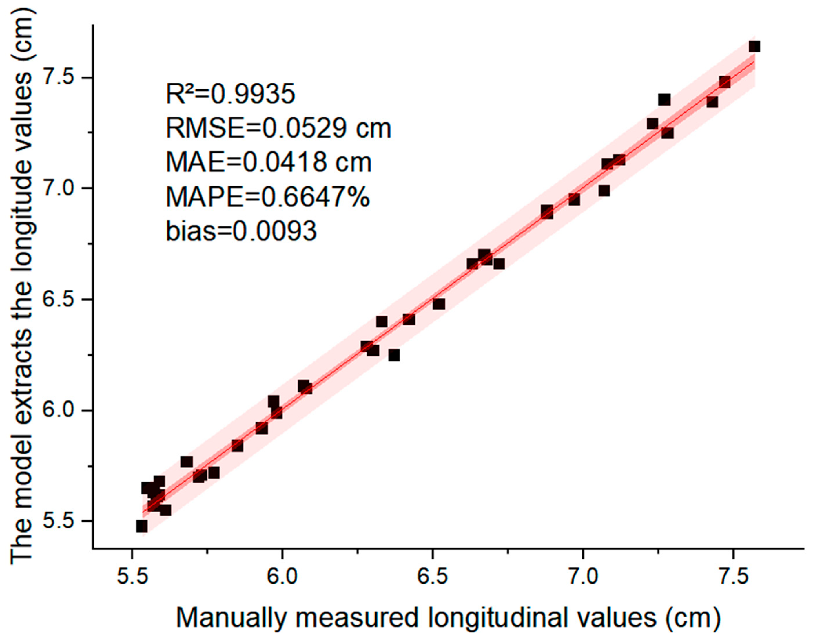
The manually measured maximum longitudinal diameters ranged from 5.53 to 7.57 cm, whereas the model-derived values ranged from 5.48 to 7.64 cm. The mean manual reference value and mean model-derived value were 6.3635 cm and 6.3728 cm, respectively, with a mean bias of 0.0093 cm. The MAE, RMSE, and MAPE were 0.0418 cm, 0.0529 cm, and 0.6647%, respectively. The 95% confidence interval of the bias ranged from −0.0076 to 0.0261 cm, and the 95% limits of agreement ranged from −0.0941 to 0.1126 cm, indicating acceptable agreement between the model-derived and manual reference measurements within the tested size range. Therefore, the model-derived maximum longitudinal diameter showed acceptable agreement with the manual reference measurements within the tested size range.

Linear regression analysis was then performed between the manually measured longitudinal diameters and the model-extracted longitudinal diameters (Figure 15). The regression equation was as follows:

$$y=0.9973x+0.0268$$

(32)

Here, x represents the manually measured longitudinal diameter, and y represents the model-extracted longitudinal diameter.

Figure 15. Regression analysis between manually measured and model-derived maximum longitudinal diameter of garlic bulbs. The x-axis represents the manual reference measurement, and the y-axis represents the value extracted from the reconstructed three-dimensional model. The solid line indicates the fitted regression line, and the shaded region indicates the 95% confidence interval of the fitted regression. n = 40.

Figure 15. Regression analysis between manually measured and model-derived maximum longitudinal diameter of garlic bulbs. The x-axis represents the manual reference measurement, and the y-axis represents the value extracted from the reconstructed three-dimensional model. The solid line indicates the fitted regression line, and the shaded region indicates the 95% confidence interval of the fitted regression. n = 40.

The model-extracted and manually measured longitudinal diameters showed a high degree of linear agreement, with the data points mainly distributed around the fitted line. This indicates that the values extracted from the 3D model accurately reflected the trend of the manual reference measurements. The regression analysis showed that the coefficient of determination (R²) was 0.9935, indicating a very strong linear correlation between the model-extracted and manual reference measurements. The root mean square error (RMSE) was 0.0529 cm, indicating that the absolute error between the model-extracted and manual reference measurements was small. The mean absolute percentage error (MAPE) was 0.6647%, which was below 1%, indicating that the method had low relative error across garlic samples of different sizes and demonstrated good measurement stability. Considering the combined results of R², RMSE, and MAPE, the proposed method can accurately extract the longitudinal diameter of garlic bulbs and demonstrates high fitting accuracy and reliability in practical measurements.

To further evaluate the appropriateness of the regression model and determine whether the model errors exhibited systematic bias, residual diagnostic analysis was performed on the longitudinal diameter extraction results.

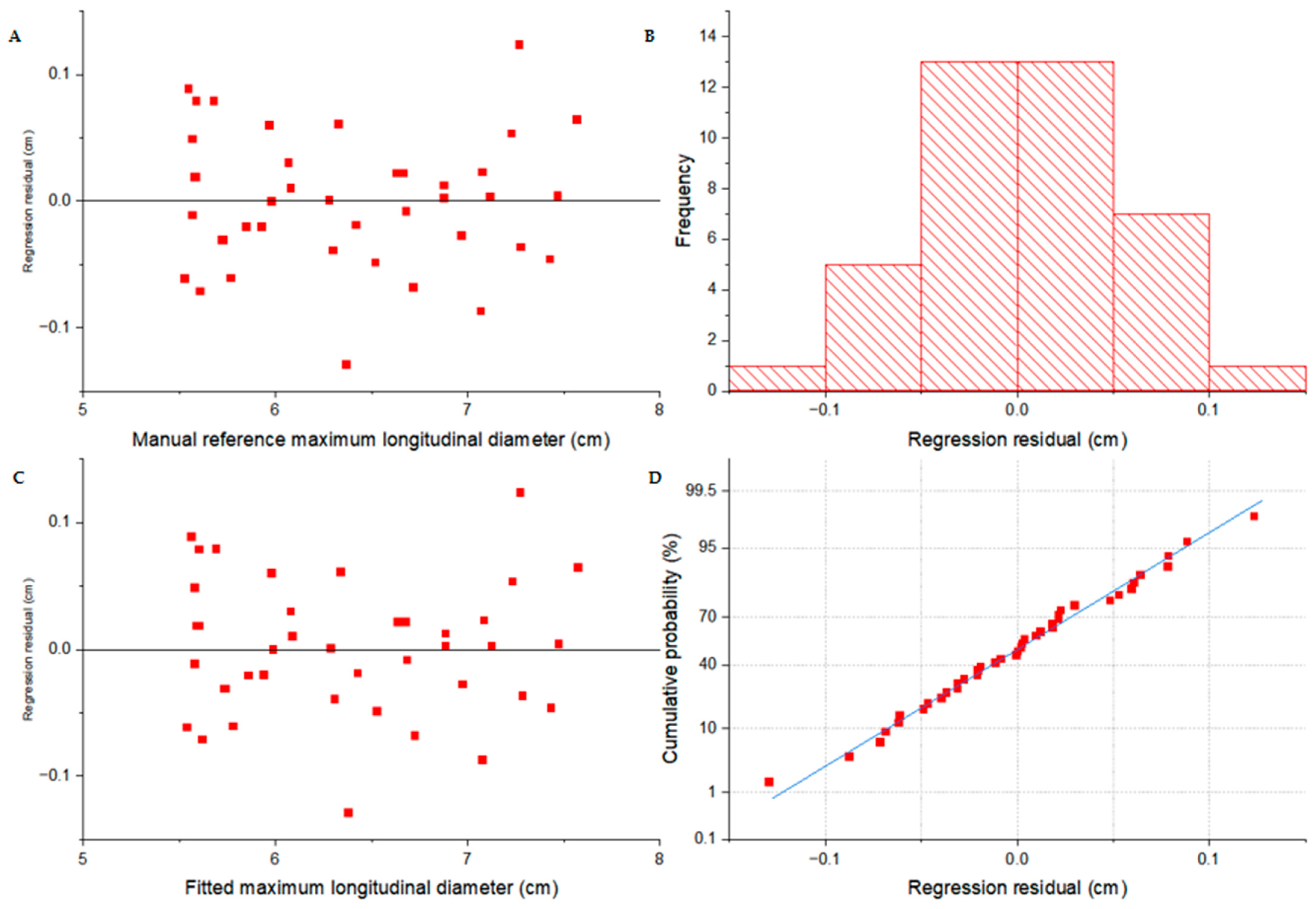
Residual diagnostic analysis was further performed to visually evaluate the fitting stability of the model for maximum longitudinal diameter extraction, as shown in Figure 16.

Figure 16A shows the relationship between residuals and manual reference measurements. Although a few residual points deviated relatively far from the zero line, most residuals were distributed on both sides of zero without an obvious monotonic trend or systematic shift. This visually suggests that the fitting errors were generally stable across the tested longitudinal diameter range.

Figure 16B shows the residual histogram. Most residuals were concentrated near zero, although a small number of samples were located at both tails and the distribution was not perfectly symmetrical. Therefore, the histogram was used only as descriptive evidence of the concentration of residuals, rather than as statistical evidence of residual normality.

Figure 16C shows the relationship between residuals and fitted values. The residuals were mainly scattered around the zero line, and no obvious funnel-shaped expansion or contraction pattern was observed. This visually suggests that the dispersion of residuals did not change markedly across the fitted-value range.

Figure 16D shows the normal probability plot of the residuals. Most points were located close to the reference line, indicating that the residual distribution did not show a pronounced departure from the expected linear pattern. Slight deviations were observed at the tails, suggesting that a small number of samples had relatively larger residuals.

Overall, the residual diagnostic plots showed that the residuals for maximum longitudinal diameter were generally distributed around zero, with no obvious systematic pattern or visually apparent variance instability.

3.2. Accuracy of Transverse Diameter Extraction

Following the same manual reference measurement and parameter-extraction procedures described above, paired maximum transverse diameter values were obtained for the 40 validation samples. For each sample, the residual and absolute percentage error were calculated from the difference between the manual reference measurement and the model-derived measurement. To keep the main text concise, the complete paired data for individual samples, including manual reference values, model-derived values, residuals, and absolute percentage errors, are provided in Supplementary Table S2. Therefore, the main manuscript focuses on the summarized error statistics, agreement analysis, and regression relationship for maximum transverse diameter.

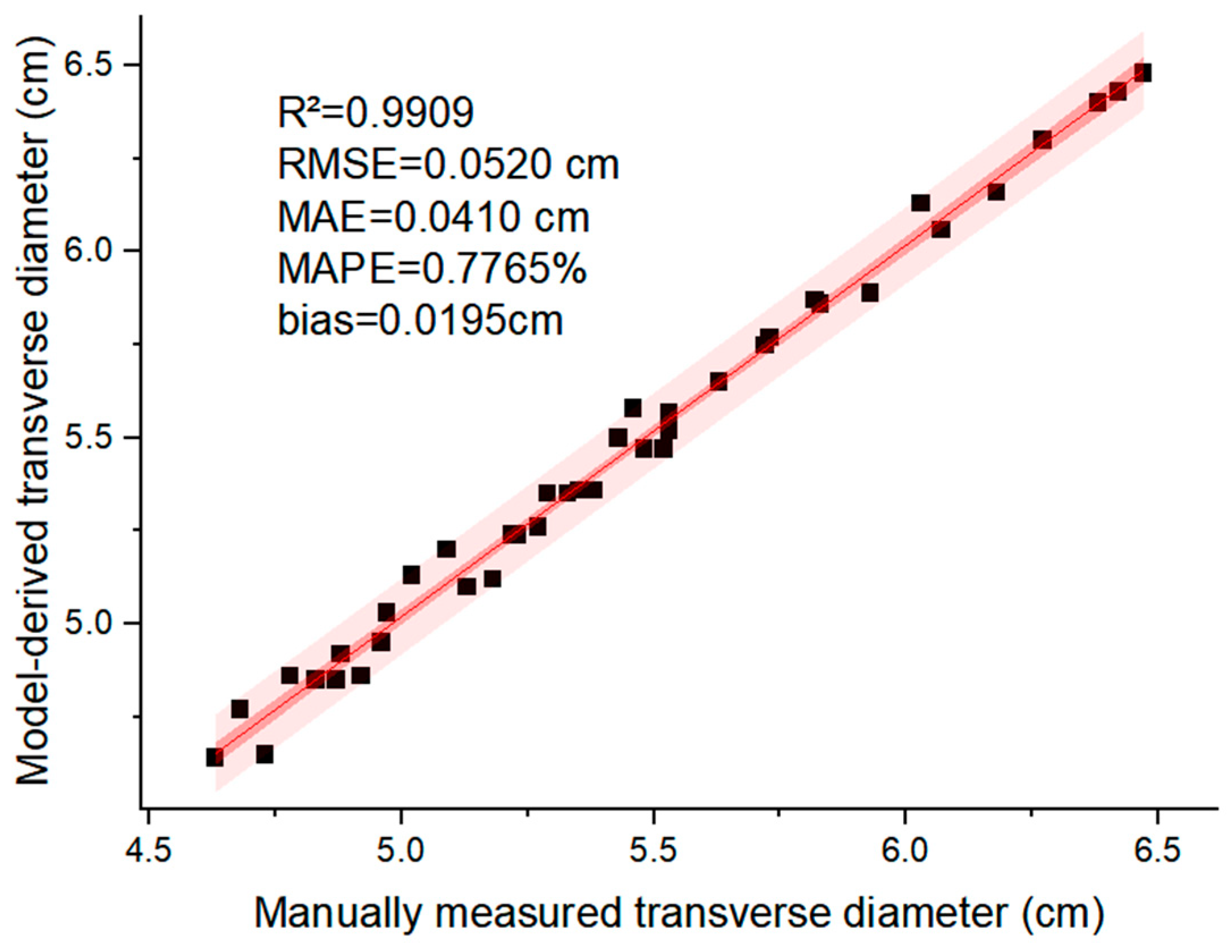
The results showed that the manually measured maximum transverse diameters ranged from 4.63 to 6.47 cm, whereas the model-derived values ranged from 4.64 to 6.48 cm, indicating that the two measurement ranges were generally consistent. The mean manual reference value was 5.4293 cm, and the mean model-derived value was 5.4488 cm, with a mean bias of 0.0195 cm. The MAE, RMSE, and MAPE were 0.0410 cm, 0.0520 cm, and 0.7765%, respectively. The 95% confidence interval of the bias ranged from 0.0039 to 0.0351 cm, and the 95% limits of agreement ranged from −0.0761 to 0.1151 cm. These results indicate that the deviations between manual reference and model-derived maximum transverse diameter measurements were small, and no obvious systematic overestimation or underestimation was observed within the tested diameter range. Overall, the distribution of errors suggests that the differences between manual and model-derived transverse diameter measurements were generally limited within the tested diameter range.

Linear regression analysis was then performed between the manually measured transverse diameters and the model-extracted transverse diameters (Figure 17). The regression equation was as follows:

$$y=0.9982x+0.0293$$

(33)

Here, x represents the manually measured transverse diameter, and y represents the transverse diameter extracted from the model.

Figure 17. Regression analysis between manually measured and model-derived maximum transverse diameters of garlic bulbs. The x-axis represents the manual reference measurement, and the y-axis represents the value extracted from the reconstructed three-dimensional model. Diameter is expressed in cm. The solid line indicates the fitted linear regression, and the shaded band indicates the 95% confidence interval of the fitted regression. R², RMSE, MAE, MAPE, and bias are shown in the panel. n = 40.

Figure 17. Regression analysis between manually measured and model-derived maximum transverse diameters of garlic bulbs. The x-axis represents the manual reference measurement, and the y-axis represents the value extracted from the reconstructed three-dimensional model. Diameter is expressed in cm. The solid line indicates the fitted linear regression, and the shaded band indicates the 95% confidence interval of the fitted regression. R², RMSE, MAE, MAPE, and bias are shown in the panel. n = 40.

The regression slope for transverse diameter was close to 1, and 38 of the 40 paired differences fell within the 95% limits of agreement. This indicates that the model-derived transverse diameter followed the manual reference measurements over the tested range.

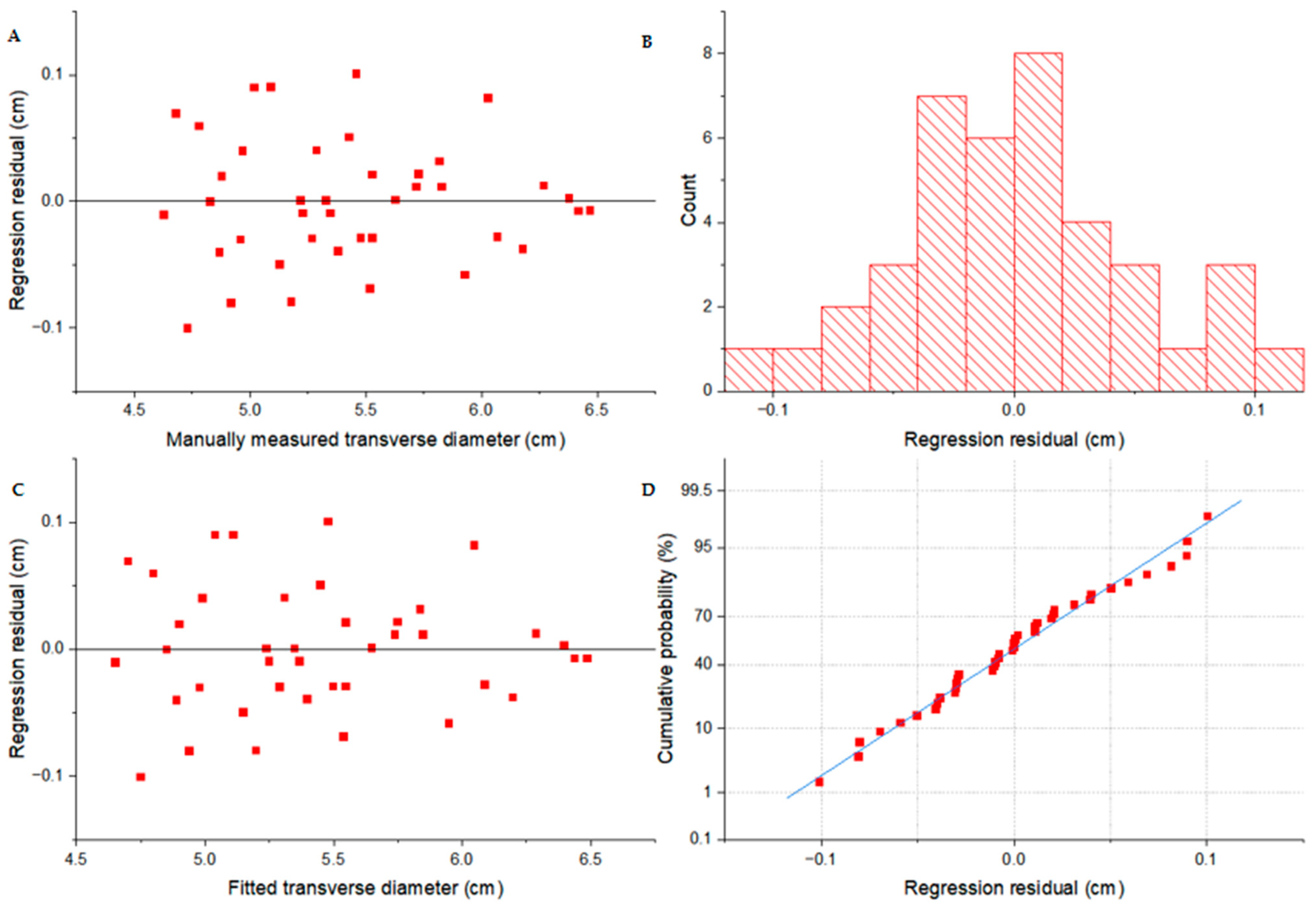
To assess the adequacy of the linear regression model and examine the structure of the regression residuals, residual diagnostic analysis was performed (Figure 18).

Residual diagnostic analysis was further performed to visually evaluate the fitting stability of the model for maximum transverse diameter extraction, as shown in Figure 18.

Figure 18A shows the relationship between residuals and manual reference measurements. The residuals were mainly distributed around the zero line, with most values falling within approximately −0.10 to 0.10 cm. Although several points in the middle transverse-diameter range showed relatively larger deviations, no obvious monotonic increasing or decreasing trend was observed. This visually suggests that the fitting errors did not show a clear systematic shift across the tested transverse diameter range.

Figure 18B shows the residual histogram. Most residuals were concentrated near zero, indicating that the majority of model-derived transverse diameter values were close to the manual reference measurements. The distribution was not perfectly symmetrical and showed a small number of samples at both tails, suggesting that a few samples had relatively larger positive or negative deviations.

Figure 18C shows the relationship between residuals and fitted values. The residuals were mainly scattered around the zero line across the fitted transverse diameter range. No obvious funnel-shaped expansion or contraction pattern was observed, suggesting that the dispersion of residuals did not change markedly with the fitted values.

Figure 18D shows the normal probability plot of the residuals. Most points were located close to the reference line, indicating that the central part of the residual distribution followed the expected linear pattern reasonably well. Slight deviations were observed at both tails, suggesting that a small number of samples contributed to relatively larger residuals.

Overall, the residual diagnostic plots showed that the residuals for maximum transverse diameter were generally distributed around zero, with no obvious systematic pattern or visually apparent variance instability. These results provide descriptive evidence that the model maintained relatively stable fitting performance for maximum transverse diameter within the tested sample range.

3.3. Accuracy of Volume Extraction

Before the accuracy validation of model-derived garlic bulb volume, the modified displacement method was verified using three rigid steel spheres with known volumes of 25, 40, and 55 cm³. As shown in

Table 2. Control verification of the modified displacement method using calibration objects with known volumes.

Calibration Object	Reference Volume (cm3)	Repeated Measured Values (cm3)	Measured Volume, Mean ± SD (cm3)	Absolute Error (cm3)	Relative Error (%)	CV (%)
Steel sphere 1	25.00	24.74, 25.04, 25.23, 24.12, 25.78	24.98 ± 0.61	0.02	0.07	2.45
Steel sphere 2	40.00	39.60, 40.17, 41.05, 38.93, 39.51	39.85 ± 0.80	0.15	0.37	2.01
Steel sphere 3	55.00	54.27, 55.61, 53.91, 56.14, 54.45	54.88 ± 0.95	0.12	0.23	1.73
Mean				0.10	0.22	2.07

Note: The measured volume was obtained using the same wrapping, vacuum-sealing, immersion, and wrapping-material correction procedure as that used for garlic bulbs. SD represents the sample standard deviation of five repeated measurements. CV represents the coefficient of variation.

, the displacement-derived volumes were close to the known reference volumes. The absolute errors of the three steel spheres ranged from 0.02 to 0.15 cm³, and the relative errors ranged from 0.07% to 0.37%. The mean absolute error and mean relative error were 0.10 cm³ and 0.22%, respectively. The coefficients of variation of the five repeated measurements ranged from 1.73% to 2.45%, with a mean value of 2.07%.

These results indicate that the mean deviation introduced by film wrapping, residual trapped air, vacuum sealing, and water-level reading was small under the experimental conditions. Although minor variability existed among repeated water-displacement readings, the use of five repeated measurements and their mean value reduced the influence of random measurement error. Therefore, the modified displacement method was considered appropriate for obtaining manual reference volumes for validating model-derived garlic bulb volume.

To evaluate the performance of the proposed method for garlic bulb volume measurement, paired volume values were obtained for the 40 validation samples using both the manual reference method and the reconstructed three-dimensional models. For each sample, the residual and absolute percentage error were calculated from the difference between the manual reference measurement and the model-derived measurement. To keep the main text concise, the complete paired data for individual samples, including manual reference values, model-derived values, residuals, and absolute percentage errors, are provided in Supplementary Table S3. Therefore, the main manuscript focuses on the summarized error statistics, agreement analysis, and regression relationship for garlic bulb volume.

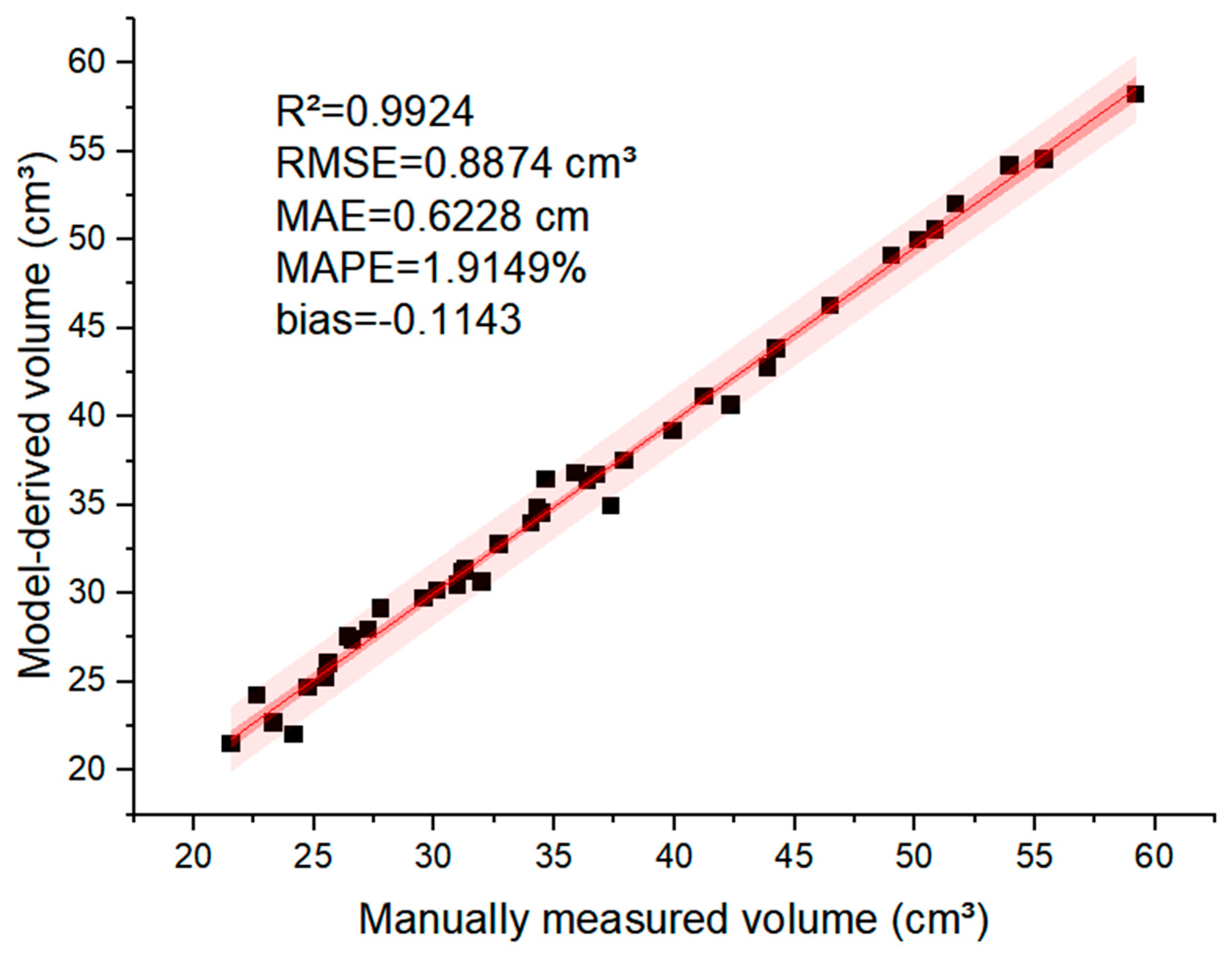
The results showed that the manually measured volumes ranged from 21.56 to 59.18 cm³, whereas the model-derived volumes ranged from 21.47 to 58.21 cm³, indicating that the two measurement ranges were generally consistent. The mean manual reference value was 36.1005 cm³, and the mean model-derived value was 35.9863 cm³, with a mean bias of −0.1143 cm³. The MAE, RMSE, and MAPE were 0.6228 cm³, 0.8874 cm³, and 1.9149%, respectively. The 95% confidence interval of the bias ranged from −0.3993 to 0.1708 cm³, and the 95% limits of agreement ranged from −1.8610 to 1.6325 cm³. These results indicate that the deviations between manual reference and model-derived volume measurements were generally small, although several individual samples showed relatively larger deviations within the tested volume range.

Linear regression analysis was further performed between the manually measured volumes and the model-extracted volumes (Figure 19). The regression equation was as follows:

$$y=0.9779x+0.6850$$

(34)

Here, x represents the manually measured volume, and y represents the model-extracted volume.

Figure 19. Relationship between manually measured and model-derived garlic bulb volumes. Black square markers represent the paired observations. The thin solid red line represents the linear regression fit, the dark-red shaded band represents the 95% confidence interval, and the light-red shaded band represents the 95% prediction interval. R², RMSE, MAE, MAPE and bias are shown in the panel. n = 40.

Figure 19. Relationship between manually measured and model-derived garlic bulb volumes. Black square markers represent the paired observations. The thin solid red line represents the linear regression fit, the dark-red shaded band represents the 95% confidence interval, and the light-red shaded band represents the 95% prediction interval. R², RMSE, MAE, MAPE and bias are shown in the panel. n = 40.

The regression analysis yielded an R² of 0.9924, indicating a close linear relationship between the manually measured and model-derived volumes. The RMSE was 0.8874 cm³, the MAE was 0.6228 cm³, and the MAPE was 1.9149%. The bias was −0.1143 cm³, with a 95% confidence interval ranging from −0.3993 to 0.1708 cm³. Because this confidence interval included zero, no clear systematic overestimation or underestimation was observed for volume measurement. The 95% limits of agreement ranged from −1.8610 to 1.6325 cm³, with 37 of the 40 paired differences falling within these limits. The magnitude of the bias was small relative to the tested volume range, and no clear size-dependent pattern was evident in the measurement differences. These results suggest that the model-derived garlic bulb volumes showed acceptable agreement with the manual reference measurements under the tested conditions.

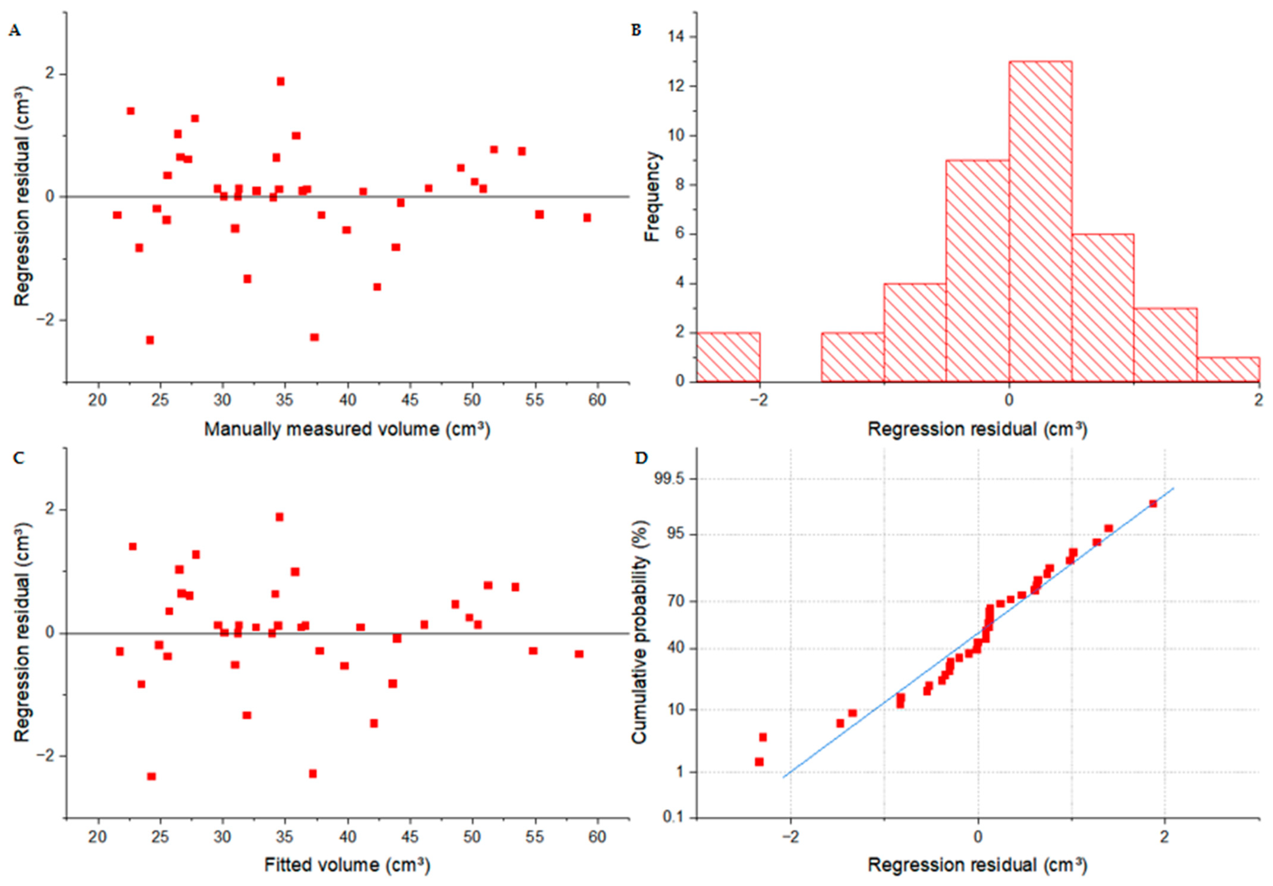
To examine the adequacy of the linear regression model and the distribution of the regression residuals, residual diagnostic analysis was performed (Figure 20).

Residual diagnostic analysis was further performed to visually evaluate the fitting stability of the model for garlic bulb volume measurement, as shown in Figure 20.

Figure 20A shows the relationship between residuals and manual reference volume. The residuals were mainly distributed around the zero line, with most values falling within approximately −2.5 to 2.0 cm³. Several samples in the smaller and middle volume ranges showed relatively larger deviations, whereas the residuals in the larger volume range were generally closer to zero. No obvious monotonic increasing or decreasing trend was observed across the tested volume range, suggesting that the volume estimation errors did not show a clear systematic shift with increasing manual reference volume.

Figure 20B shows the residual histogram. Most residuals were concentrated near zero, especially within the range of approximately −1.0 to 1.0 cm³, indicating that most model-derived volume values were close to the manual reference measurements. However, the distribution was not perfectly symmetrical, and a small number of samples appeared at both tails, particularly in the negative residual range. This suggests that several individual samples had relatively larger deviations in volume estimation.

Figure 20C shows the relationship between residuals and fitted values. The residuals were mainly scattered around the zero line across the fitted volume range. Although several points with relatively large negative residuals were observed in the lower and middle fitted-volume ranges, no obvious funnel-shaped expansion or contraction pattern was observed. This visually suggests that the dispersion of residuals did not change markedly with the fitted volume values.

Figure 20D shows the normal probability plot of the residuals. Most points were located close to the reference line in the central region of the distribution, indicating that the central residual pattern was generally consistent with the expected linear trend. Slight deviations were observed at both tails, especially for a few negative residuals, suggesting that a small number of samples contributed to relatively larger volume estimation errors.

Overall, the residual diagnostic plots showed that the residuals for garlic bulb volume were generally distributed around zero, with no obvious systematic pattern or visually apparent variance instability. The relatively larger deviations observed in a few samples may be related to the sensitivity of volume estimation to local surface reconstruction quality, basal-region processing, and small point-cloud voids. These results provide descriptive evidence that the proposed method maintained acceptable fitting stability for garlic bulb volume measurement within the tested sample range.

3.4. Bland–Altman Agreement and Morphology-Based Error Analysis

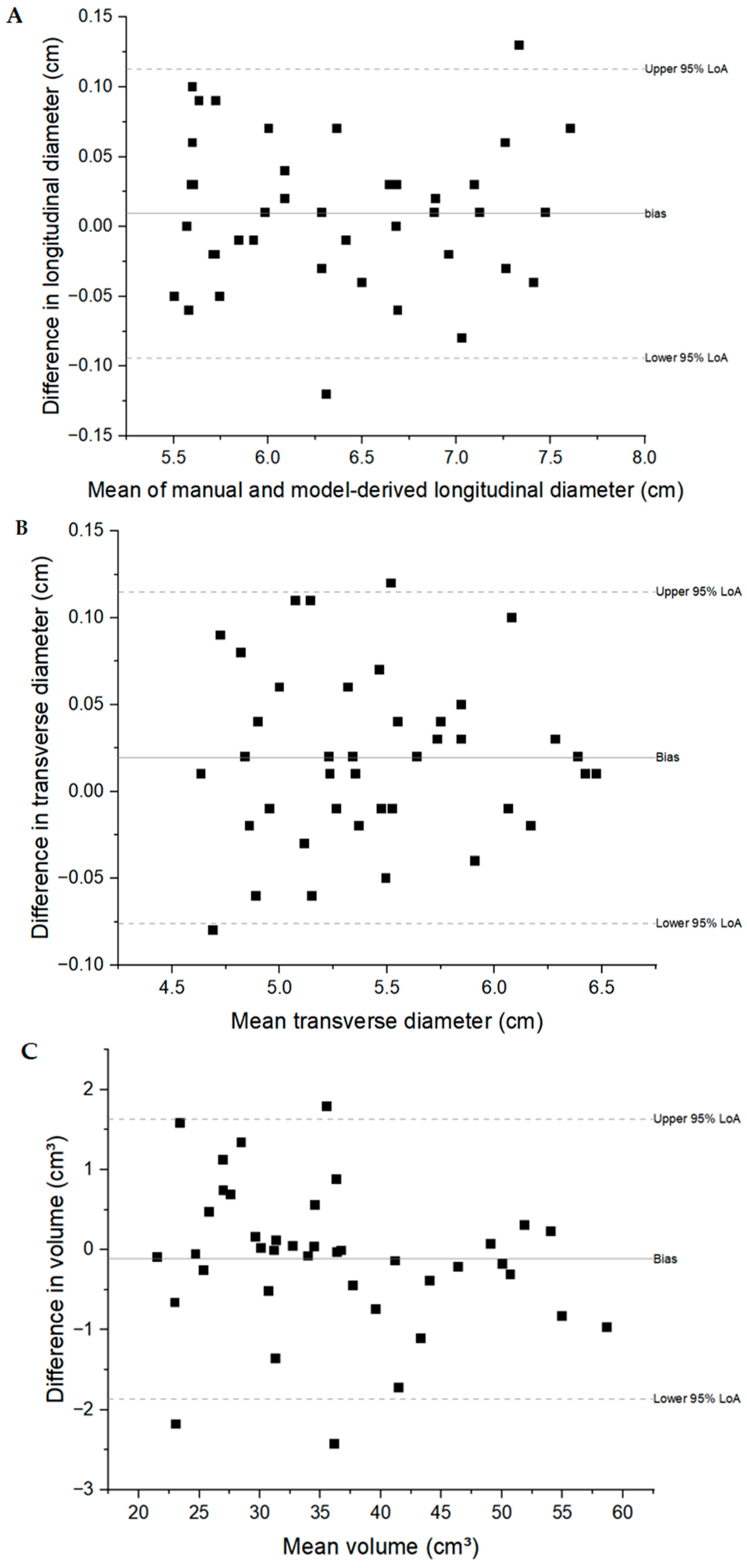
Although the regression results demonstrated strong linear relationships between the manually measured and model-derived values, regression analysis alone is not sufficient to confirm the agreement between two measurement methods. Therefore, Bland–Altman analysis was further performed to evaluate systematic bias and the distribution of measurement differences for maximum longitudinal diameter, maximum transverse diameter, and volume. In this analysis, the difference was calculated as the model-derived value minus the manually measured value.

As shown in Figure 21, the paired differences for the three phenotypic traits were mainly distributed around the mean bias line, and most observations fell within the corresponding 95% limits of agreement. For maximum longitudinal diameter and volume, the 95% confidence intervals of the bias included zero, indicating that no obvious systematic overestimation or underestimation was observed. For maximum transverse diameter, the bias was slightly positive, suggesting a weak tendency of overestimation; however, the magnitude of this deviation was small relative to the measured transverse-diameter range of the validation samples. Overall, the Bland–Altman results indicate that the model-derived measurements were in good agreement with the manual reference measurements under the tested conditions.

The distribution of differences also showed no obvious increasing or decreasing trend with increasing mean value, suggesting that the measurement errors were not strongly size-dependent within the tested range. Compared with the two diameter traits, volume showed a wider range of differences. This was expected because volume estimation is more sensitive to cumulative surface deviations in the reconstructed point cloud, especially around irregular clove boundaries, local epidermal folds, basal clipping regions, and small depressions between adjacent cloves. Therefore, although the volume measurement maintained a low relative error overall, it was more easily affected by local reconstruction imperfections than the diameter measurements.

To further examine whether bulb morphology affected measurement accuracy, morphology-based error analysis was conducted by grouping the 40 validation samples according to bulb size and bulb shape. Bulb size was classified based on manually measured volume, whereas bulb shape was characterized using the shape index, calculated as the ratio of maximum longitudinal diameter to maximum transverse diameter. The grouped error statistics are summarized in

Table 3. Morphology-based error analysis of model-derived phenotypic measurements according to bulb size and shape index.

Grouping Criterion	Group	n	Range	Longitudinal Diameter MAE (cm)	Longitudinal Diameter MAPE (%)	Transverse Diameter MAE (cm)	Transverse Diameter MAPE (%)	Volume MAE (cm3)	Volume MAPE (%)
Bulb size based on manual volume	Small	13	21.56–30.12 cm3	0.0500	0.8818	0.0515	1.0508	0.7208	2.8702
Bulb size based on manual volume	Medium	13	31.00–37.37 cm3	0.0315	0.5017	0.0354	0.6588	0.6062	1.7466
Bulb size based on manual volume	Large	14	37.93–59.18 cm3	0.0436	0.6146	0.0364	0.6309	0.5471	1.1840
Shape index	Low	14	1.0495–1.1625	0.0357	0.5843	0.0443	0.8456	0.4250	1.3347
Shape index	Medium	13	1.1628–1.1876	0.0477	0.7749	0.0408	0.8085	0.6915	2.4633
Shape index	High	13	1.1898–1.2210	0.0423	0.6412	0.0377	0.6699	0.7669	1.9913

Note: Shape index was calculated as the ratio of maximum longitudinal diameter to maximum transverse diameter. Bulb-size groups were defined according to manually measured volume. MAPE represents the mean absolute percentage error between model-derived and manual reference measurements.

.

Across the bulb-size groups, the measurement errors for the maximum longitudinal and transverse diameters were generally low and relatively stable. For volume estimation, both the MAE and MAPE were higher in the small-bulb group than in the medium- and large-bulb groups. The volume MAPE decreased from 2.8702% in the small-bulb group to 1.7466% in the medium-bulb group and 1.1840% in the large-bulb group. This pattern may be partly attributable to the smaller reference volumes of small bulbs, for which a comparable absolute deviation results in a larger percentage error. However, because the small-bulb group also exhibited a slightly higher volume MAE, volume estimation for smaller bulbs may have been more sensitive than diameter estimation to local surface reconstruction errors and boundary effects within the tested range.

The shape-index-based analysis indicated that the proposed method showed relatively stable diameter measurement performance across bulbs with different morphological characteristics. The errors in the maximum longitudinal and transverse diameters did not show a clear increasing trend from the low to the high shape-index group. Specifically, the longitudinal diameter error was highest in the medium shape-index group rather than in the high shape-index group, whereas the transverse diameter error decreased slightly as the shape index increased. These findings suggest that the PCA-based pose correction and contour-based diameter extraction may have helped reduce the influence of shape variation on diameter measurement.

For volume estimation, the MAE increased from the low to the high shape-index group, whereas the MAPE was highest in the medium shape-index group and did not increase monotonically with the shape index. Thus, although some group-level variation in volume error was observed, no clear consistent shape-dependent pattern was observed simultaneously in the absolute and relative error metrics. Overall, the grouped analyses suggested that the proposed multi-view reconstruction and point-cloud processing workflow showed a certain degree of robustness to variations in garlic bulb size and shape within the validation set.

4. Discussion

4.1. Interpretation of the Measurement Accuracy

This study evaluated whether multi-view image reconstruction combined with point-cloud processing could provide reliable non-destructive measurements of key external phenotypic traits of garlic bulbs. Within the investigated validation range, the model-derived measurements showed close agreement with the manual reference measurements. The coefficients of determination for maximum longitudinal diameter, maximum transverse diameter, and volume were 0.9935, 0.9909, and 0.9924, respectively, while the corresponding RMSE values were 0.0529 cm, 0.0520 cm, and 0.8874 cm³. The MAPE values were 0.6647%, 0.7765%, and 1.9149%, respectively. Together with the small MAE and bias values, these results indicate that the proposed workflow can characterize dimensional and volumetric variation among garlic bulbs with relatively low measurement error.

The results support the basic premise of this study that complete multi-view surface information can be used to extract garlic bulb traits that are difficult to characterize comprehensively using conventional two-dimensional images. In particular, the point-cloud representation preserves the spatial distribution of the bulb surface and therefore enables both linear dimensions and volume to be quantified within the same measurement framework. The similar performance obtained for maximum longitudinal diameter and maximum transverse diameter also suggests that the pose-correction procedure effectively standardized the spatial orientation of the reconstructed bulbs before trait extraction.

The relative error of volume estimation was higher than those of the two diameter measurements. This difference is reasonable because maximum longitudinal and transverse diameters are determined mainly by specific contour points or geometric boundaries, whereas volume calculation depends on the completeness and geometric fidelity of the entire reconstructed surface. Small local deviations in point-cloud density, surface reconstruction, basal cropping, or raster integration may have only a limited effect on linear measurements but can accumulate during whole-surface volume calculation. Garlic bulbs also contain clove boundaries, local depressions, epidermal folds, and irregular curved surfaces, which increase the geometric complexity of volume reconstruction. Nevertheless, the average MAPE of volume remained below 2%, indicating that the method retained useful three-dimensional characterization capability for the evaluated bulbs.

The relatively low error in maximum longitudinal diameter may also be associated with the contour-constrained extraction method developed in this study. Because part of the basal point cloud was removed together with the supporting structure during preprocessing, direct calculation based only on the maximum and minimum Z coordinates could underestimate the actual longitudinal diameter. The triangular contour constraint reconstructed the effective longitudinal height from the basal endpoints and the bulb apex, thereby reducing the influence of the incomplete basal boundary. This targeted treatment of the basal region represents an important methodological feature of the workflow and improves its suitability for garlic bulbs with partially occluded bases.

Although the high R² values demonstrate strong linear relationships, measurement performance should not be interpreted on the basis of correlation alone. Therefore, the reliability of the proposed workflow is more appropriately supported by the combined evidence from R², RMSE, MAE, MAPE, bias, regression slope, intercept, confidence intervals, and Bland–Altman limits of agreement. The Bland–Altman results showed that most paired differences fell within the 95% limits of agreement, indicating acceptable agreement between model-derived and manual reference measurements under the tested conditions. The residual diagnostic plots also showed no obvious systematic trend over the investigated measurement ranges, suggesting that the errors were not concentrated only in small or large bulbs. However, statements regarding residual normality or heteroscedasticity should remain cautious unless supported by formal statistical tests.

4.2. Comparison with Previous 3D Phenotyping Methods

Three-dimensional crop phenotyping has been conducted using LiDAR, structured-light scanning, CT or micro-CT imaging, and image-based photogrammetry. LiDAR is effective for acquiring three-dimensional coordinates and measuring canopy height, tiller number, and plant structural traits under field conditions [5,6]. Structured-light systems can capture detailed surface geometry under controlled conditions [7], whereas CT and micro-CT imaging provide detailed external and internal structural information. However, these methods often require specialized equipment, controlled environments, limited sample sizes, or relatively time-consuming scanning procedures [8].

Image-based photogrammetry reconstructs three-dimensional geometry from overlapping images acquired at multiple viewing angles. Previous studies have applied this approach to wheat seedlings, sweet potato plants, tomato plants and fruits, and other crop structures, mainly focusing on plant architecture, canopy traits, leaf traits, or aboveground growth parameters [10,11,12,13,14]. Compared with these targets, garlic bulbs are compact storage organs with irregular outlines, pronounced clove boundaries, epidermal folds, local depressions, and heterogeneous surface texture, which create specific challenges for feature matching, point-cloud completion, and geometric trait extraction.

Recent studies on compact or storage organs provide useful references, but they differ from the present study in target organ, imaging system, and extracted traits. For garlic cloves, previous work used depth-camera-derived three-dimensional features to predict clove volume and mass, demonstrating the usefulness of 3D information for irregular garlic organs. In contrast, the present study focuses on whole garlic bulbs rather than individual cloves, and extracts grading-related bulb traits from photogrammetric point clouds [35]. For sweet potato storage roots, low-cost 3D scanning has been used to directly quantify surface area and volume of elongated storage roots, showing the value of 3D geometry for evaluating traits related to processing performance. By comparison, garlic bulbs are more compact and have clearer clove boundaries, epidermal folds, and local depressions; therefore, the present workflow emphasizes multi-view image reconstruction, point-cloud preprocessing, and pose correction for whole-bulb geometric measurement [36]. For radish roots, three-dimensional image analysis combined with machine learning has been applied to estimate root weight, indicating that reconstructed root geometry can support biomass-related trait prediction. The present study differs in that it does not rely on machine-learning prediction of biomass, but instead directly extracts maximum longitudinal diameter, maximum transverse diameter, and volume from standardized point clouds for garlic bulb assessment [37]. For saffron organs, a low-cost dual-camera photogrammetric workflow has been developed for organ-level 3D phenotyping, showing that passive multi-view imaging can be adapted to complex crop organs. Similarly, the present study uses passive image-based reconstruction, but it further adapts the workflow to whole garlic bulbs by integrating controlled turntable-based image acquisition, photogrammetric reconstruction, point-cloud preprocessing, pose correction, and trait extraction according to GB/T 45244-2025 [15,30].

Overall, compared with previous studies on garlic cloves, sweet potato storage roots, radish roots, and saffron organs, the value of the present study lies in adapting image-based three-dimensional phenotyping to intact garlic bulbs and establishing a complete workflow for grading-related trait extraction. By extracting maximum longitudinal diameter, maximum transverse diameter, and volume from the same standardized point cloud according to the requirements of GB/T 45244-2025 [15], the proposed method provides a unified framework for non-destructive garlic bulb assessment. Compared with active three-dimensional sensing methods used in some previous storage-organ studies, this workflow uses a conventional digital camera, a motorized turntable, and controlled illumination instead of specialized laser, depth, or tomographic equipment. This configuration is flexible for laboratory-based phenotyping and can acquire both geometric and texture information. Nevertheless, the proposed method should be regarded as a complementary approach rather than a replacement for existing three-dimensional sensing techniques. Further comparison of equipment cost, acquisition time, processing efficiency, and measurement performance is still needed before drawing conclusions about its relative economy or efficiency.

4.3. Factors Affecting Reconstruction and Measurement Accuracy

The measurement accuracy obtained in this study was influenced by both image-acquisition conditions and subsequent point-cloud processing. During image acquisition, the use of a matte background, controlled side illumination, a fixed turntable step, and high overlap between adjacent images helped reduce background interference and provided sufficient correspondences for multi-view reconstruction. Capturing images after the turntable had stopped also reduced motion blur and angular deviation. These measures contributed to the completeness and geometric consistency of the reconstructed bulb surfaces.

Nevertheless, garlic surface characteristics remain an important source of reconstruction uncertainty. Areas with weak texture may provide insufficient features for image matching, whereas reflective or shadowed regions may generate inconsistent pixel information among different viewing angles. Pronounced clove boundaries and folds may also produce abrupt local depth changes. These effects can result in uneven point density or small local voids, particularly around depressed regions and narrow gaps between cloves. The limited number of samples with relatively large volume errors may therefore be associated with irregular bulb shapes, local surface depressions, or incomplete reconstruction of complex boundaries.

The basal region represents another potential source of uncertainty. Fixing the bulb in the sample holder improved acquisition stability but partially obscured the basal contour. In addition, the RANSAC-based plane removal and Z-axis pass-through filtering used to eliminate the supporting structure could remove a small proportion of valid basal points. The contour-constrained longitudinal-diameter method reduced the influence of this incomplete boundary, whereas volume estimation remained more sensitive because it depends on the entire reconstructed surface. Future optimization of sample fixation and basal-region reconstruction may further improve volume accuracy without reducing acquisition stability.

Although the illumination environment was controlled and images were saved in RAW format, variations in image brightness, colour consistency, or local reflections may still affect feature matching and reconstruction quality, especially for bulbs with different skin colours and epidermal characteristics. In the revised acquisition protocol, fixed exposure parameters, locked white balance, and unified RAW conversion settings were used to reduce radiometric differences among views. Further sensitivity analyses of image number, angular interval, voxel size, denoising parameters, and cropping thresholds would help determine which settings have the greatest influence on reconstruction completeness and trait-extraction accuracy.

Uncertainty in the manual reference measurements should also be considered when interpreting differences between the two methods. The use of a digital caliper with repeated measurements reduced random errors in maximum longitudinal and transverse diameter measurements. For volume, wrapping and vacuum sealing were used to prevent water absorption, and the volume of the wrapping material was subtracted from the total displacement. The control verification using rigid steel spheres with known volumes showed small absolute and relative errors, supporting the reliability of the modified displacement method under the experimental conditions. However, small uncertainties may remain because of film thickness, residual air, deformation during vacuum sealing, and water-level reading.

4.4. Implications for Garlic Grading and Germplasm Evaluation

Garlic bulb size and morphology are important for yield-related evaluation, commercial classification, and processing suitability [4]. Maximum longitudinal diameter, maximum transverse diameter, and volume are important external morphological traits for garlic bulb characterization, grading-related assessment, and germplasm evaluation. Conventional manual measurements require repeated physical contact and may be affected by operator judgment, particularly when bulb contours are irregular. The proposed workflow provides digital three-dimensional records of individual bulbs and extracts multiple traits from the same model, which may improve data traceability and support repeated or retrospective phenotypic analysis.

The present results demonstrate the feasibility of the workflow under controlled laboratory conditions and provide a methodological basis for future garlic phenotyping and grading systems. The reconstructed point clouds could also support the extraction of additional traits, such as shape index, surface curvature, asymmetry, clove-boundary characteristics, and local deformation. Consequently, the framework may be extended beyond the three parameters evaluated here to provide a more comprehensive description of garlic bulb morphology.

The current quantitative validation was conducted using 40 Lanling white-skinned garlic bulbs, while the other three garlic materials were used to demonstrate the applicability of multi-view reconstruction to bulbs with different external appearances. This design was appropriate for validating the proposed measurement workflow under a consistent reference dataset, but cultivar-specific measurement accuracy was not statistically evaluated in the present study. Future studies should include balanced validation datasets across multiple cultivars to further evaluate the effects of skin colour, surface texture, clove boundary characteristics, and bulb morphology on reconstruction accuracy.

The morphology-based error analysis showed that the proposed method maintained relatively stable measurement performance across different bulb-size and shape-index groups within the validation set. Volume error was slightly higher in the small-bulb group than in the medium- and large-bulb groups, which may be explained by the greater influence of similar absolute deviations on relative error for smaller samples. The shape-index-based analysis did not show a clear increasing error trend from low to high shape-index groups, suggesting that the PCA-based pose correction and contour-based diameter extraction reduced the influence of moderate shape variation on measurement accuracy.

4.5. Limitations and Future Work

Several aspects should be further addressed in future studies to improve the generalizability and practical applicability of the workflow. First, although four garlic materials were included to demonstrate reconstruction feasibility, quantitative validation was performed using one representative cultivar. A larger and more diverse dataset including more cultivars, wider size ranges, different skin colours, stronger clove-boundary variation, and more irregular bulb morphologies would further strengthen the evaluation of robustness.

Second, all reconstruction and point-cloud processing parameters were fixed before the final accuracy validation and were applied consistently to the 40 validation samples. No sample-specific, size-specific, shape-specific, or trait-specific parameter tuning was performed during validation. This fixed protocol supports the repeatability of the reported validation results. Future studies could further adopt independent calibration and validation datasets, or cross-validation procedures, to evaluate the generalization performance of the workflow more rigorously.

Third, the present study focused primarily on measurement accuracy under controlled laboratory conditions. Before large-scale or industrial deployment, acquisition time, reconstruction time, point-cloud processing throughput, failure rate, hardware and software requirements, and robustness under practical grading conditions should be systematically evaluated. These evaluations would clarify the balance between accuracy and efficiency and support comparison with existing manual or automated grading approaches.

Finally, greater automation of point-cloud segmentation, preprocessing, and trait extraction would facilitate integration with continuous grading or online inspection equipment. Overall, this study establishes a coherent image-based framework for non-destructive three-dimensional measurement of garlic bulbs. By adapting multi-view reconstruction and point-cloud analysis to the morphological characteristics of a bulbous organ and linking the extracted parameters to grading-related standards, the study provides both a technical contribution to crop phenotyping and a foundation for further development of automated garlic assessment systems.

5. Conclusions

This study developed a non-destructive three-dimensional phenotypic measurement workflow for garlic bulbs based on multi-view imaging, photogrammetric reconstruction, and point-cloud processing. The workflow integrated standardized image acquisition, three-dimensional reconstruction, point-cloud cropping, denoising, downsampling, pose correction, and targeted extraction of maximum longitudinal diameter, maximum transverse diameter, and volume. By adapting the processing procedure to the morphological characteristics of garlic bulbs, the method provided a complete technical framework for extracting grading-related external traits from reconstructed point clouds.

Quantitative validation was conducted using 40 Lanling white-skinned garlic bulbs, with manual measurements used as reference values. The model-derived measurements showed close agreement with manual reference measurements. The R² values for maximum longitudinal diameter, maximum transverse diameter, and volume were 0.9935, 0.9909, and 0.9924, respectively. The corresponding RMSE values were 0.0529 cm, 0.0520 cm, and 0.8874 cm³, and the MAPE values were 0.6647%, 0.7765%, and 1.9149%, respectively. The additional MAE, bias, confidence interval, and Bland–Altman analyses further indicated that the deviations between model-derived and manual measurements were generally small under the tested conditions.

The main scientific contribution of this study is the establishment of a garlic-bulb-oriented three-dimensional phenotyping workflow that links multi-view reconstruction with national-standard-related morphological parameter extraction. Compared with conventional manual measurements, the proposed workflow provides digital three-dimensional records and enables multiple external traits to be extracted from the same reconstructed model. These results demonstrate the feasibility of using image-based three-dimensional reconstruction for non-destructive garlic bulb phenotypic measurement.

The present study provides a methodological basis for future garlic phenotyping, germplasm evaluation, and grading-related assessment. However, further work is still needed before large-scale or industrial application, including validation with larger and more diverse cultivar populations, evaluation of acquisition and processing throughput, comparison with existing grading methods, and improvement of automated point-cloud segmentation and parameter extraction. These future developments will help enhance the robustness, efficiency, and practical applicability of the proposed workflow.

References

1. Ezeorba, T.P.C.; Ezugwu, A.L.; Chukwuma, I.F.; Anaduaka, E.G.; Udenigwe, C.C. Health-promoting properties of bioactive proteins and peptides of garlic (Allium sativum). Food Chem. 2024, 435, 137632. [Google Scholar] [CrossRef] [Scilit] [PubMed]
2. Sunanta, P.; Kontogiorgos, V.; Pankasemsuk, T.; Jantanasakulwong, K.; Rachtanapun, P.; Seesuriyachan, P.; Sommano, S.R. The nutritional value, bioactive availability and functional properties of garlic and its related products during processing. Front. Nutr. 2023, 10, 1142784. [Google Scholar] [CrossRef] [Scilit] [PubMed]
3. Liu, P.; Wang, Y.; Xu, Y.; Weng, R.; Qiu, J.; Qian, Y. Monitoring changes in biochemical and metabolite profiles in garlic cloves during storage. J. Agric. Food Chem. 2024, 72, 10117–10126. [Google Scholar] [CrossRef] [Scilit] [PubMed]
4. Choudhary, S.; Choudhary, B.; Kumhar, S. Genetic variability in the garlic (Allium sativum) genotypes for growth, yield and yield attributing traits. Ann. Plant Soil Res. 2017, 19, 115–120. [Google Scholar]
5. Friedli, M.; Kirchgessner, N.; Grieder, C.; Liebisch, F.; Mannale, M.; Walter, A. Terrestrial 3D laser scanning to track the increase in canopy height of both monocot and dicot crop species under field conditions. Plant Methods 2016, 12, 9. [Google Scholar] [CrossRef] [Scilit] [PubMed]
6. Fang, Y.; Qiu, X.; Guo, T.; Wang, Y.; Cheng, T.; Zhu, Y.; Chen, Q.; Cao, W.; Yao, X.; Niu, Q. An automatic method for counting wheat tiller number in the field with terrestrial LiDAR. Plant Methods 2020, 16, 132. [Google Scholar] [CrossRef] [Scilit] [PubMed]
7. Nguyen, T.T.; Slaughter, D.C.; Max, N.; Maloof, J.N.; Sinha, N. Structured light-based 3D reconstruction system for plants. Sensors 2015, 15, 18587–18612. [Google Scholar] [CrossRef] [Scilit] [PubMed]
8. Karahara, I.; Yamauchi, D.; Uesugi, K.; Mineyuki, Y. Three-dimensional visualization of plant tissues and organs by X-ray micro–computed tomography. Microscopy 2023, 72, 310–325. [Google Scholar] [CrossRef] [Scilit] [PubMed]
9. Kolhar, S.; Jagtap, J. Plant trait estimation and classification studies in plant phenotyping using machine vision—A review. Inf. Process. Agric. 2023, 10, 114–135. [Google Scholar] [CrossRef] [Scilit]
10. Lou, L.; Liu, Y.; Han, J.; Doonan, J.H. Accurate multi-view stereo 3D reconstruction for cost-effective plant phenotyping. In Proceedings of the International Conference Image Analysis and Recognition; Springer: Berlin/Heidelberg, Germany, 2014; pp. 349–356. [Google Scholar]
11. Duan, T.; Chapman, S.; Holland, E.; Rebetzke, G.; Guo, Y.; Zheng, B. Dynamic quantification of canopy structure to characterize early plant vigour in wheat genotypes. J. Exp. Bot. 2016, 67, 4523–4534. [Google Scholar] [CrossRef] [Scilit] [PubMed]
12. Zhang, Y.; Teng, P.; Aono, M.; Shimizu, Y.; Hosoi, F.; Omasa, K. 3D monitoring for plant growth parameters in field with a single camera by multi-view approach. J. Agric. Meteorol. 2018, 74, 129–139. [Google Scholar] [CrossRef] [Scilit]
13. Wang, Y.; Hu, S.; Ren, H.; Yang, W.; Zhai, R. 3DPhenoMVS: A low-cost 3D tomato phenotyping pipeline using 3D reconstruction point cloud based on multiview images. Agronomy 2022, 12, 1865. [Google Scholar] [CrossRef] [Scilit]
14. Li, B.; Wu, Q.; Wu, J.; Zhang, M.; Li, H.; Yu, K.; Cao, J.; Zhang, W.; Cao, H.; Zhang, W. Optimization of crop 3D point cloud reconstruction strategy based on the multi-view automatic imaging system. Trans. Chin. Soc. Agric. Eng. 2023, 39, 161–171. [Google Scholar] [CrossRef]
15. GB/T 45244-2025; Grades and Specifications of Garlic. State Administration for Market Regulation; Standardization Administration of China: Beijing, China, 2025.
16. Yang, W.; Zhang, Y.; Ye, J.; Ji, Y.; Li, Z.; Zhou, M.; Yu, J. Structure from motion on XSlit cameras. IEEE Trans. Pattern Anal. Mach. Intell. 2019, 43, 1691–1704. [Google Scholar] [CrossRef] [PubMed]
17. Zhou, H.; Jagadeesan, J. Real-time dense reconstruction of tissue surface from stereo optical video. IEEE Trans. Med. Imaging 2019, 39, 400–412. [Google Scholar] [CrossRef] [Scilit] [PubMed]
18. Ahmed, S.; Hansard, M.; Cavallaro, A. Constrained optimization for plane-based stereo. IEEE Trans. Image Process. 2018, 27, 3870–3882. [Google Scholar] [CrossRef] [PubMed]
19. Yang, S.; Han, J.Y.; Lim, S.-H.; Kim, S.; Lee, J.; Kim, K.-S.; Kim, J.-M.; Yi, W.-J. DCrownFormer+: Morphology-aware mesh generation and refinement transformer for dental crown prosthesis from 3D scan data of preparation and antagonist teeth. Med. Image Anal. 2025, 105, 103717. [Google Scholar] [CrossRef] [Scilit] [PubMed]
20. Mu, W.; Li, Y.; Deng, M.; Han, N.; Guo, X. Crop Leaf Phenotypic Parameter Measurement Based on the RKM-D Point Cloud Method. Sensors 2024, 24, 1998. [Google Scholar] [CrossRef] [Scilit] [PubMed]
21. Lou, M.; Lu, J.; Wang, L.; Jiang, H.; Zhou, M. Growth parameter acquisition and geometric point cloud completion of lettuce. Front. Plant Sci. 2022, 13, 947690. [Google Scholar] [CrossRef] [Scilit] [PubMed]
22. Pan, D.; Liu, B.; Luo, L.; Zeng, A.; Zhou, Y.; Pan, K.; Xian, Z.; Xian, Y.; Liu, L. A dual-task segmentation network based on multi-head hierarchical attention for 3D plant point cloud. Front. Plant Sci. 2025, 16, 1610443. [Google Scholar] [CrossRef] [Scilit] [PubMed]
23. Wang, F.; Zhu, T.; Huang, L.; Feng, C.; Lu, X.; Min, W.; Wang, Z.; Hu, X.; Nie, Y. VGDS-PointNet++ for organ segmentation and phenotypic trait estimation in greenhouse tomato seedlings. Front. Plant Sci. 2026, 17, 1753706. [Google Scholar] [CrossRef] [Scilit] [PubMed]
24. Qiao, G.; Zhang, Z.; Niu, B.; Han, S.; Yang, E. Plant stem and leaf segmentation and phenotypic parameter extraction using neural radiance fields and lightweight point cloud segmentation networks. Front. Plant Sci. 2025, 16, 1491170. [Google Scholar] [CrossRef] [Scilit] [PubMed]
25. Gené-Mola, J.; Sanz-Cortiella, R.; Rosell-Polo, J.R.; Escola, A.; Gregorio, E. In-field apple size estimation using photogrammetry-derived 3D point clouds: Comparison of 4 different methods considering fruit occlusions. Comput. Electron. Agric. 2021, 188, 106343. [Google Scholar] [CrossRef] [Scilit]
26. Ma, H.; Wang, K.; Ma, J.; Jiang, S.; Liu, P.; Yang, C.; Wang, D.; Cui, H.; Chang, H. Calculation method of canopy effective volume for fruit tree based on LiDAR point cloud data. Front. Plant Sci. 2025, 16, 1679027. [Google Scholar] [CrossRef] [Scilit] [PubMed]
27. Wang, H.; Blok, P.M.; Burridge, J.; Jiang, T.; Miyauchi, M.; Miyamoto, K.; Tanaka, K.; Guo, W. 3DPotatoTwin: A paired potato tuber dataset for 3D multi-sensory fusion. Plant Phenomics 2025, 7, 100123. [Google Scholar] [CrossRef] [Scilit] [PubMed]
28. Yuan, D.; Hu, X.; Zhang, H.; Jia, W.; Mao, Z.-H.; Sun, M. An automatic electronic instrument for accurate measurements of food volume and density. Public Health Nutr. 2021, 24, 1248–1255. [Google Scholar] [CrossRef] [Scilit] [PubMed]
29. Liu, B.; Li, X.; Liang, Z.; Liu, Y.; Zou, X. CotSkNet: Semantic segmentation of point clouds and phenotypic trait extraction for fragile organs in densely planted cotton under field conditions. Inf. Process. Agric. 2026; in press. [CrossRef] [Scilit]
30. Huang, X.; Jiang, H.; Wan, X.; Chen, C.; Nie, W.; Zhou, T.; Pei, J.; Peng, C. Organ-level 3D phenotyping of saffron using a low-cost dual-camera workflow. Plant Methods 2026, 22, 24. [Google Scholar] [CrossRef] [Scilit] [PubMed]
31. Hodson, T.O. Root mean square error (RMSE) or mean absolute error (MAE): When to use them or not. Geosci. Model Dev. Discuss. 2022, 15, 5481–5487. [Google Scholar] [CrossRef] [Scilit]
32. Santiago, G.N.; Cisdeli Magalhaes, P.H.; Carcedo, A.J.; Marziotte, L.; Mayor, L.; Ciampitti, I.A. Deep learning methods using imagery from a smartphone for recognizing sorghum panicles and counting grains at a plant level. Plant Phenomics 2024, 6, 0234. [Google Scholar] [CrossRef] [Scilit] [PubMed]
33. Kim, S.; Xin, X.; Kim, S.-Y.; Kim, G.; Baek, M.-g.; Won, D.Y.; Baek, C.H.; Kim, G. De-occlusion models and diffusion-based data augmentation for size estimation of on-plant oriental melons. Plant Phenomics 2025, 7, 100097. [Google Scholar] [CrossRef] [Scilit] [PubMed]
34. Berrigan, E.M.; Wang, L.; Carrillo, H.; Echegoyen, K.; Kappes, M.; Torres, J.; Ai-Perreira, A.; Mccoy, E.; Shane, E.; Copeland, C.D. Fast and efficient root phenotyping via pose estimation. Plant Phenomics 2024, 6, 0175. [Google Scholar] [CrossRef] [Scilit] [PubMed]
35. Son, J.-H.; Park, H.-G.; Han, Y.-J.; Kang, S.-H.; Woo, S.-M.; Ha, Y.-S. Prediction of garlic clove volume and mass using a depth camera and machine learning models. Postharvest Biol. Technol. 2025, 226, 113526. [Google Scholar] [CrossRef] [Scilit]
36. Villordon, A.; Gregorie, J.C.; LaBonte, D. Direct Measurement of Sweetpotato Surface Area and Volume Using a Low-cost 3D Scanner for Identification of Shape Features Related to Processing Product Recovery. HortScience 2020, 55, 722–728. [Google Scholar] [CrossRef] [Scilit]
37. Kamiwaki, Y.; Fukuda, S. A Machine Learning-Assisted Three-Dimensional Image Analysis for Weight Estimation of Radish. Horticulturae 2024, 10, 142. [Google Scholar] [CrossRef] [Scilit]
Figure 1. Representative samples of the four garlic cultivars used in this study. (A) Pizhou single-clove garlic; (B) Pizhou white-top garlic; (C) Yunnan purple-skinned garlic; (D) Lanling white-skinned garlic. The four garlic materials were selected to represent different bulb morphologies, skin colours, and external surface characteristics. One representative bulb is shown for each material to illustrate differences in bulb morphology, skin colour, and external surface characteristics.
Horticulturae 12 00887 g001
Figure 2. Overall workflow of non-destructive three-dimensional phenotyping of garlic bulbs based on multi-view imaging. The workflow includes image acquisition, photogrammetric three-dimensional reconstruction, point-cloud preprocessing, phenotypic parameter extraction, manual ground-truth measurement, and accuracy validation. Multi-view images were acquired using a controlled imaging platform and reconstructed into three-dimensional models. The reconstructed point clouds were processed through cropping, denoising, voxel downsampling, and pose correction before extracting maximum longitudinal diameter, maximum transverse diameter, and volume. Model-derived measurements were compared with manual reference measurements using regression analysis and agreement analysis. Solid arrows indicate the direction of data processing. The differently coloured boxes represent image acquisition, three-dimensional reconstruction, point-cloud processing, phenotypic measurement, and accuracy validation, respectively. Dashed frames indicate the major workflow stages.
Horticulturae 12 00887 g002
Figure 3. Image acquisition preparation and system configuration for multi-view imaging of garlic bulbs. (A) Low-reflection optical acquisition environment constructed using a matte black background to reduce stray light and background interference. (B) Side-illumination setup using a Godox SL60 LED continuous light source positioned at an oblique angle of approximately 45° to reduce shadows and surface reflections. (C) TurntableX parameter settings for controlled turntable rotation. (D) Timer-triggered shutter release used to capture images after the turntable reached a stationary position. The same imaging configuration was used for all validation samples.
Horticulturae 12 00887 g003
Figure 4. Representative multi-view image datasets of garlic bulbs used for three-dimensional reconstruction. (A) Pizhou single-clove garlic dataset; (B) Pizhou white-top garlic dataset; (C) Yunnan purple-skinned garlic dataset; (D) Lanling white-skinned garlic dataset. One representative bulb is shown for each material. For each bulb, 24 images were acquired at 15° intervals over a full 360° rotation. These multi-view images were used as input data for photogrammetric reconstruction.
Horticulturae 12 00887 g004aHorticulturae 12 00887 g004b
Figure 5. Photogrammetric three-dimensional reconstruction workflow implemented in ContextCapture. The workflow includes EXIF data extraction, camera parameter correction, lens distortion correction, SIFT–RANSAC feature matching, SfM-based sparse reconstruction, bundle adjustment, PatchMatch-based dense matching, Poisson surface reconstruction, mesh filtering and hole filling, texture mapping, colour balancing, and OBJ model export. The final three-dimensional models were used for subsequent point-cloud processing and phenotypic parameter extraction. Red, green, purple, and yellow indicate the four main stages of the reconstruction workflow, respectively: camera parameter correction, SfM triangulation, dense point-cloud and mesh construction, and model optimization and texturing. Within each stage, the lighter-colored boxes represent the specific processing steps or algorithms. The colors are used only for visual classification and do not represent quantitative values.
Horticulturae 12 00887 g005
Figure 6. Reconstructed point-cloud models of representative garlic bulbs generated from multi-view images. (A) Pizhou single-clove garlic; (B) Pizhou white-top garlic; (C) Yunnan purple-skinned garlic; (D) Lanling white-skinned garlic. The models were reconstructed in ContextCapture and exported in OBJ format. These examples demonstrate that the multi-view imaging workflow can reconstruct garlic bulbs with different skin colours, clove boundary characteristics, and external morphologies.
Horticulturae 12 00887 g006
Figure 7. Point-cloud cropping of reconstructed garlic bulb models. (A) Raw reconstructed point cloud before cropping, containing the garlic bulb, supporting pot, substrate, and background-related outliers. (B) Cropped garlic bulb point cloud after RANSAC plane fitting and Z-axis pass-through filtering. One representative point cloud is shown to illustrate the cropping procedure. Point-cloud dimensions were processed in the calibrated model coordinate system.
Horticulturae 12 00887 g007
Figure 8. Effect of voxel grid downsampling on the garlic bulb point cloud. (A) Before model downsampling; (B) After downsampling the model. One representative point cloud is shown to illustrate the effect of point-cloud simplification.
Horticulturae 12 00887 g008
Figure 9. Pose correction of the garlic bulb point cloud using principal component analysis. (A) Garlic bulb point cloud before pose correction, showing spatial inclination relative to the coordinate system. (B) Garlic bulb point cloud after PCA-based pose correction, with the principal longitudinal axis aligned with the spatial Z-axis. This standardized orientation was used for consistent extraction of maximum longitudinal diameter, maximum transverse diameter, and volume.
Horticulturae 12 00887 g009
Figure 10. Extraction of maximum transverse diameter from the reconstructed garlic bulb model. The maximum transverse diameter was determined from the widest horizontal contour of the pose-corrected point cloud in the XY plane. The extracted transverse diameter is expressed in cm. One representative sample is shown to illustrate the measurement procedure.
Horticulturae 12 00887 g010
Figure 11. Extraction of maximum longitudinal diameter from the reconstructed garlic bulb model. A longitudinal cross-sectional contour was used to construct a three-point geometric constraint, where the two basal contour endpoints and the upper apex formed a triangle. The perpendicular height from the apex to the basal line was calculated as the maximum longitudinal diameter. The extracted longitudinal diameter is expressed in cm. One representative sample is shown to illustrate the measurement procedure.
Horticulturae 12 00887 g011
Figure 12. Relative height distribution map used for raster-based volume calculation of garlic bulbs. The point cloud was projected and rasterized along the growth axis, and the relative height distribution was used to calculate local volume contributions from grid cells. Green regions indicate areas where the reconstructed surface height was close to the main bulb surface, whereas yellow to red regions indicate local height deviations, mainly distributed near the basal clipping region and irregular surface boundaries.
Horticulturae 12 00887 g012
Figure 13. Manual measurement of garlic bulb diameters using a digital vernier caliper. (A) Measurement of maximum transverse diameter at the widest equatorial region of the bulb; (B) Measurement of maximum longitudinal diameter from the basal end to the apical end of the bulb. Diameter measurements are expressed in cm. One representative bulb is shown to illustrate the manual measurement procedure.
Horticulturae 12 00887 g013
Figure 14. Schematic illustration of the modified displacement method used for manual garlic bulb volume measurement. The procedure included measuring the volume of the empty wrapping material, wrapping and vacuum-sealing the garlic bulb, immersing the wrapped bulb in water, recording the liquid-level rise, and subtracting the wrapping-material volume from the total displacement volume. Each bulb was measured in triplicate, and the mean value was used as the manual reference volume. Unit: cm3.
Horticulturae 12 00887 g014
Figure 16. Residual diagnostic plots for the linear regression between manually measured and model-derived maximum longitudinal diameters. (A) Residuals versus manually measured longitudinal diameter; (B) histogram of residuals; (C) residuals versus fitted values; (D) normal probability plot of residuals. Red square markers represent the residuals of individual samples, the red hatched bars represent the frequency distribution of the residuals, the solid horizontal line indicates zero residual, and the blue diagonal line in the normal probability plot represents the theoretical normal reference line. Residuals were calculated as model-derived values minus manual reference values. Diameter residuals are expressed in cm. The horizontal zero line indicates no difference between the two methods. n = 40.
Horticulturae 12 00887 g016
Figure 18. Residual diagnostic plots for the linear regression between manually measured and model-derived maximum transverse diameters. (A) Residuals versus manually measured transverse diameter; (B) Histogram of residuals; (C) Residuals versus fitted values; (D) Normal probability plot of residuals. Red square markers represent the residuals of individual samples, the red hatched bars represent the frequency distribution of the residuals, the solid horizontal line indicates zero residual, and the blue diagonal line in the normal probability plot represents the theoretical normal reference line. Residuals were calculated as model-derived values minus manual reference values. Diameter residuals are expressed in cm. n = 40.
Horticulturae 12 00887 g018
Figure 20. Residual diagnostic plots for the linear regression between manually measured and model-derived garlic bulb volumes. (A) Residuals versus manually measured volume; (B) Histogram of residuals; (C) Residuals versus fitted values; (D) Normal probability plot of residuals. Red square markers represent the residuals of individual samples, the red hatched bars represent the frequency distribution of the residuals, the solid horizontal line indicates zero residual, and the blue diagonal line in the normal probability plot represents the theoretical normal reference line. Volume residuals are expressed in cm3. n = 40.
Horticulturae 12 00887 g020
Figure 21. Bland–Altman plots showing the agreement between manually measured and model-derived garlic bulb phenotypic traits. (A) Maximum longitudinal diameter; (B) maximum transverse diameter; (C) volume. The x-axis represents the mean of the manually measured and model-derived values, and the y-axis represents the difference calculated as model-derived value minus manually measured value. Black square markers represent the paired differences for individual garlic bulb samples. The solid horizontal line indicates the mean bias, and the dashed horizontal lines indicate the upper and lower 95% limits of agreement. n = 40.
Horticulturae 12 00887 g021