Calculation and Prediction of Water Requirements for Aeroponic Cultivation of Crops in Greenhouses

Abstract

Crop aeroponic cultivation still faces issues such as insufficient precision in water supply control and scientifically-based irrigation scheduling. To address this challenge, the present study aims to establish a precision irrigation protocol adapted to the characteristics of crop aeroponic cultivation. Using coriander (Coriandrum sativum L.) as the experimental subject, crop water requirements were estimated utilizing both the FAO56 P-M equation and its revised form. The RMSE between the water requirement measured values and the calculated values using the P-M formula is 2.12 mm, the MAE is 2.0 mm, and the MAPE is 14.29%. The RMSE between the water requirement measured values and the calculated values using the revised P-M formula is 0.88 mm, the MAE is 0.82 mm, and the MAPE is 5.78%. The results indicate that the water requirement values calculated using the revised P-M formula are closer to the measured values. For model development, this study used coriander evapotranspiration as a basis. Major environmental variables influencing water requirement were selected as input features, and the daily reference water requirement served as the output. Three modeling approaches were implemented: Random Forest (RF), Bagging, and M5P Model Tree algorithms. The results indicate that, in comparing various input combinations (C1: air temperature, relative humidity, atmospheric pressure, wind speed, radiation, photoperiod; C2: air temperature, relative humidity, wind speed, radiation; C3: air temperature, relative humidity, radiation), the RF model based on C1 input demonstrated superior performance with RMSE = 0.121 mm/d, MAE = 0.134 mm/d, MAPE = 2.123%, and R² = 0.971. It significantly outperforms the RF models with other input combinations, as well as the Bagging and M5P models across all input scenarios, in terms of convergence rate, determination coefficient, and comprehensive performance. Its predictions aligned more closely with observed data, showing enhanced accuracy and adaptability. This optimized prediction model demonstrates particular suitability for forecasting water requirements in aeroponic coriander production and provides theoretical support for efficient, intelligent water-saving management in crop aeroponic cultivation.

1. Introduction

Prediction of crop water requirements forms the foundational basis for scientific irrigation scheduling, yet the calculation process is inherently complex [1,2]. Crop water requirements are subject to the dynamic coupling of multiple factors. A shift in a single environmental parameter frequently triggers a cascade of responses in related variables. Direct measurement methods for water requirement, though accurate, present operational difficulties, are time-intensive, and incur significant costs in practical use [3]. As a result, indirect estimation methods based on climate data have become the prevailing approach for crop water requirement calculation. However, water requirement is fundamentally constrained by an array of factors, including meteorological parameters, crop varietal traits, field management practices, soil conditions, and the technical level of production [4,5]. In agricultural practice, it is essential to systematically integrate meteorological, crop, soil, and local productivity factors to analyze crop water use patterns and provide a robust scientific basis for precision irrigation decision-making [6].

Aeroponic cultivation is a modern soilless system characterized by the use of atomization equipment to deliver nutrient solution or water as a fine mist directly to crop roots. Roots remain suspended in a closed cultivation chamber, simultaneously meeting requirements for moisture and nutrients and ensuring an ample oxygen supply [7,8,9]. Its significant advantage lies in its high water utilization efficiency, as water directly affects the root system, greatly reducing ineffective consumption such as inter-row evaporation and deep percolation observed in traditional soil-based cultivation. At the same time, it eliminates soil tillage, fertilization, and other processes, significantly reducing labor intensity [10,11]. Although aeroponic cultivation has been widely applied to facility-based cultivation of vegetables, flowers, and fruit trees in regions with water scarcity or limited soil conditions due to its water-saving characteristics, there are still prominent issues in practice, such as insufficient precision in water supply regulation and a lack of scientific basis for irrigation scheduling. There is an urgent need to establish a precision irrigation system tailored to its specific characteristics. This is because, during different growth stages of crops, insufficient water supply leads to an imbalance between transpiration and root water uptake, causing leaf wilting and root damage, which in turn reduces yields. Conversely, excessive water supply results in wasted water resources. Therefore, the core of developing a rational irrigation system lies in accurately predicting crop water requirements.

Traditionally, the prediction of crop water requirements in greenhouse environments has often directly relied on the FAO56 P-M equation, which was originally developed for open-field conditions. This approach neglects the substantial influence of the enclosed greenhouse microclimate on calculation accuracy. As a result, existing models exhibit significant predictive deviations in the context of aeroponic cultivation, thereby hindering the advancement of intelligent water-saving irrigation technologies. To enhance water use efficiency and promote the intelligent development of aeroponic cultivation, there is a pressing need to develop more reliable water prediction models specifically tailored for greenhouse applications. By integrating real-time environmental monitoring data with machine learning approaches, it is possible to achieve accurate prediction of coriander water requirements without relying on conventional empirical formulas, thereby providing a data-driven foundation for precision irrigation. To accurately predict the water requirements of crops in aeroponic cultivation systems and establish a reasonable irrigation system, this study employs machine learning algorithms. Using coriander as the experimental subject, real-time environmental parameters such as air temperature, relative humidity, atmospheric pressure, wind speed, radiation, and photoperiod were collected through an intelligent environmental monitoring system within a greenhouse. Since the FAO56 P-M formula is designed for outdoor environments, and greenhouse conditions differ from these, in this study, we first applied the FAO56 P-M formula in combination with collected data to calculate the daily water requirements of coriander. The formula was then revised to account for greenhouse environmental characteristics. Finally, the calculation results from both the standard and revised formulas were compared with the measured daily water requirements, and the method with the least error was selected as the basis for subsequent water requirement prediction and irrigation system optimization. To establish an accurate daily water requirement prediction model for coriander, significant environmental parameters affecting water requirements were selected as input variables, and different parameter combinations were set based on these inputs. Random Forest (RF), M5P Model Tree, and Bagging prediction models were constructed with coriander’s daily water requirements as the output. Finally, by comparing the convergence speed, determination coefficient, and other performance indicators of model predictions against measured values for different input combinations, the optimal environmental parameter input combination and prediction model were selected. This study proposes an improved research pathway that integrates machine learning with water requirement calculation formulas. By incorporating machine learning algorithms, we systematically evaluated the impact of different environmental parameter combinations as input variables on model performance, thereby identifying the optimal prediction model and the most critical environmental drivers for coriander aeroponic cultivation. This approach provides accurate daily water requirement predictions for coriander aeroponics, offering a core algorithm and solid theoretical foundation for formulating scientific irrigation strategies and enabling efficient, intelligent, and closed-loop water-saving control.

2. Materials and Methods

2.1. Overview and Basic Conditions of the Study Area

The study area is located at Hunan Agricultural University in Changsha, Hunan Province, at 113°5′ E longitude and 28°11′ N latitude, with an elevation of approximately 46 m. The area belongs to a subtropical monsoon climate, with distinct seasons, long summers and winters, and short springs and autumns. Summer lasts for approximately 118–127 days, winter for about 117–122 days, spring for approximately 61–64 days, and autumn for about 59–69 days. According to data from the National Meteorological Station in Changsha, in 2021, the experimental area exhibited a daytime average temperature of 23 °C and a nighttime average temperature of 16 °C. The highest daily temperature reached 40.9 °C, while the lowest was −33.9 °C. Large diurnal temperature variations occurred during spring and fall. The average daily humidity was recorded at 83%. The majority of precipitation occurred from May to July, with average rainfall ranging from 150 to 250 mm and annual evaporation measured at 2100 mm. The annual average wind speed was 3.9 m/s, with a maximum of 16.0 m/s and peak gusts up to 30 m/s. Average annual sunshine hours totaled approximately 2884.8 h.

2.2. Composition of Greenhouse Crop Aeroponic Cultivation System

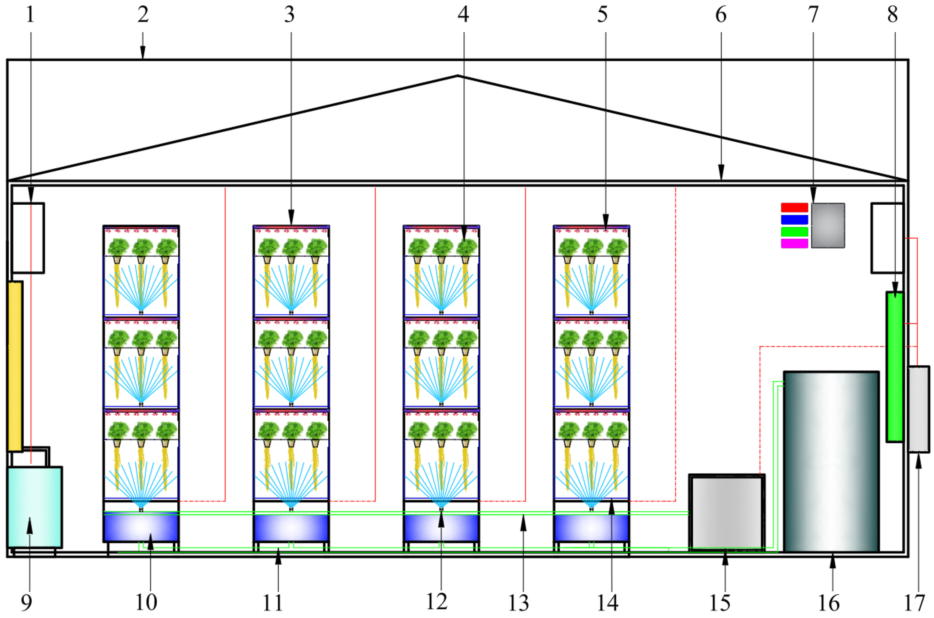
The greenhouse crop aeroponic cultivation system mainly consists of a greenhouse structure, vertical aeroponic growing units, an automated nutrient solution formulation and misting apparatus, an intelligent environmental parameter monitoring system, and auxiliary equipment. As depicted in Figure 1. The operating principle of the greenhouse aeroponic cultivation system entails placing healthy, transplant-ready seedlings into planting baskets, then installing the baskets within planting holes in cultivation panels. The automated nutrient solution regulation and misting apparatus delivers a fine spray to the root system within the cultivation box, ensuring optimal hydration and nutrient supply. Meanwhile, real-time environmental monitoring and regulation are achieved through a dedicated, intelligent sensor network.

2.3. Experimental Design

To achieve accurate calculation and prediction of coriander water requirements in greenhouse aeroponic cultivation conditions, this study defined a single growing cycle, from transplanting seedlings onto extruded polystyrene panels through harvest, as approximately 30 days. According to the timeline of the growth cycle, in this study, we distinguished four growth periods for coriander: initial stage (6 days), development stage (8 days), mid-stage (12 days), and late stage (4 days). The water consumption experiment for aeroponically grown coriander included both an experimental group and a control group. In the experimental group, the daily evapotranspiration of coriander was monitored. At 8:00 each morning, consumption of nutrient solution from the reservoir over the prior 24 h was measured using a digital electronic scale. For the control group, coriander was not cultivated. Digital weighing at 8:00 each morning quantified water loss attributable to factors other than coriander growth. By subtracting the control group results from the experimental group data, daily coriander water consumption was obtained. Water requirements were also calculated using both the FAO56 P-M equation and a revised version of the formula. Calculated daily water requirements from both methods were compared with actual measured values, and the method with lower error was identified based on these results. Subsequently, three machine learning algorithms are used: the RF, M5P, and Bagging models. Core input features included daily meteorological variables: air temperature, relative humidity, atmospheric pressure, wind speed, radiation, and sunshine duration. The output was the predicted coriander water requirement, supporting the training of the predictive models. Three different combinations of input variables were defined, as shown in

Table 1. Prediction model with different input combinations.

Model	Combination Name	Input Parameter
RF, M5P, Bagging	C1	Air temperature, Relative humidity, Atmospheric pressure, Wind speed, radiation, Light exposure time
	C2	Air temperature, Relative humidity, Wind speed, Radiation
	C3	Air temperature, Relative humidity, Radiation

. Finally, predictions for all three input combinations were generated via the M5P, RF, and Bagging models. Predicted water requirements were compared with actual observed values, and the model exhibiting the lowest error and best performance was identified. To ensure the reproducibility of the experiment, all model configurations, training, and evaluations were performed in the same computing environment on a local laptop. The specific environment is as follows: Windows 10 (64-bit) operating system, Weka 3.9 software, where M5P is the specific implementation of the M5P algorithm tree, and RF and Bagging are provided as independent “meta-classifiers” or “classifiers”. The CPU is an Intel Core i7-10510U processor (Intel Corporation, Santa Clara, CA, USA), with 16 GB of RAM. No external machine learning libraries were called upon throughout the entire process.

2.4. Cultivation Environment and Management

Coriander was selected as the experimental crop. Seedlings were cultivated using coriander seeds supplied by China Vegetable Seed Technology Co., Ltd. (Beijing, China). At the onset of seedling cultivation, coriander seeds enclosed in fruit coats were divided into two halves by manual rubbing. The crushed seeds were then soaked in warm water for 24 h. Multiple nursery trays were prepared. Each tray was lined with perforated nursery foam, which was first moistened. Soaked seeds were distributed evenly into each round aperture in the nursery foam. Water was misted onto the foam and coriander seeds 3–5 times daily to maintain a moist environment conducive to germination. After 8–15 days of cultivation, seedlings were selected based on having 4–6 leaves and root lengths between 30 and 50 mm. Vigorous and uniformly growing seedlings were fixed in planting baskets and randomly transplanted into planting holes on extruded polystyrene panels within a vertical aeroponic system. Each planting hole accommodated one coriander plant. Planting layout on each panel followed a 3-row by 6-column matrix, with 18 coriander plants per panel. Spacing between rows was 150 mm, and between columns was 183 mm, to account for canopy development and coverage characteristics. This study used six extruded polystyrene panels and a total of 108 coriander plants.

Based on preliminary aeroponic trials with coriander, misting intervals were set according to four distinct growth stages: 1 min ON/10 min OFF during the initial stage; 1 min ON/5 min OFF during the development stage; 2 min ON/5 min OFF during the mid-season stage; and 1 min ON/5 min OFF during the late-season stage. Full-spectrum LED plant growth lamps served as the lighting source. To enhance aeroponic efficiency and reduce the crop cycle, photoperiod optimization was carried out using a 24 h cycle. The photoperiod for the four growth stages was set as follows: initial stage—12 h light (06:00–18:00), 12 h dark (18:00–06:00); development stage—14 h light (06:00–20:00), 10 h dark (20:00–06:00); mid-season stage—16 h light (06:00–22:00), 8 h dark (22:00–06:00); late season stage—14 h light (06:30–20:30), 10 h dark (20:00–06:00). The light source is provided by plant growth lamps (Bohan Lighting Technology Co., Ltd., Zhongshan, Guangdong, China) with the following parameters: 220 V, 1.2 m, 28 W, photosynthetic photon flux density (PPFD) of 140 ± 10 (μmol/m²)/s. The nutrient solution during coriander growth followed the Leafy Vegetable Formula A from South China Agricultural University, nutrient solution EC value range: 1.6 ± 0.1 mS/cm (initial stage), 1.8 ± 0.1 mS/cm (development stage), 2.0 ± 0.1 mS/cm (mid-stage), 2.2 ± 0.1 mS/cm (late stage), and pH between 6.2 and 6.8 [12,13].

2.5. Meteorological Data Collection

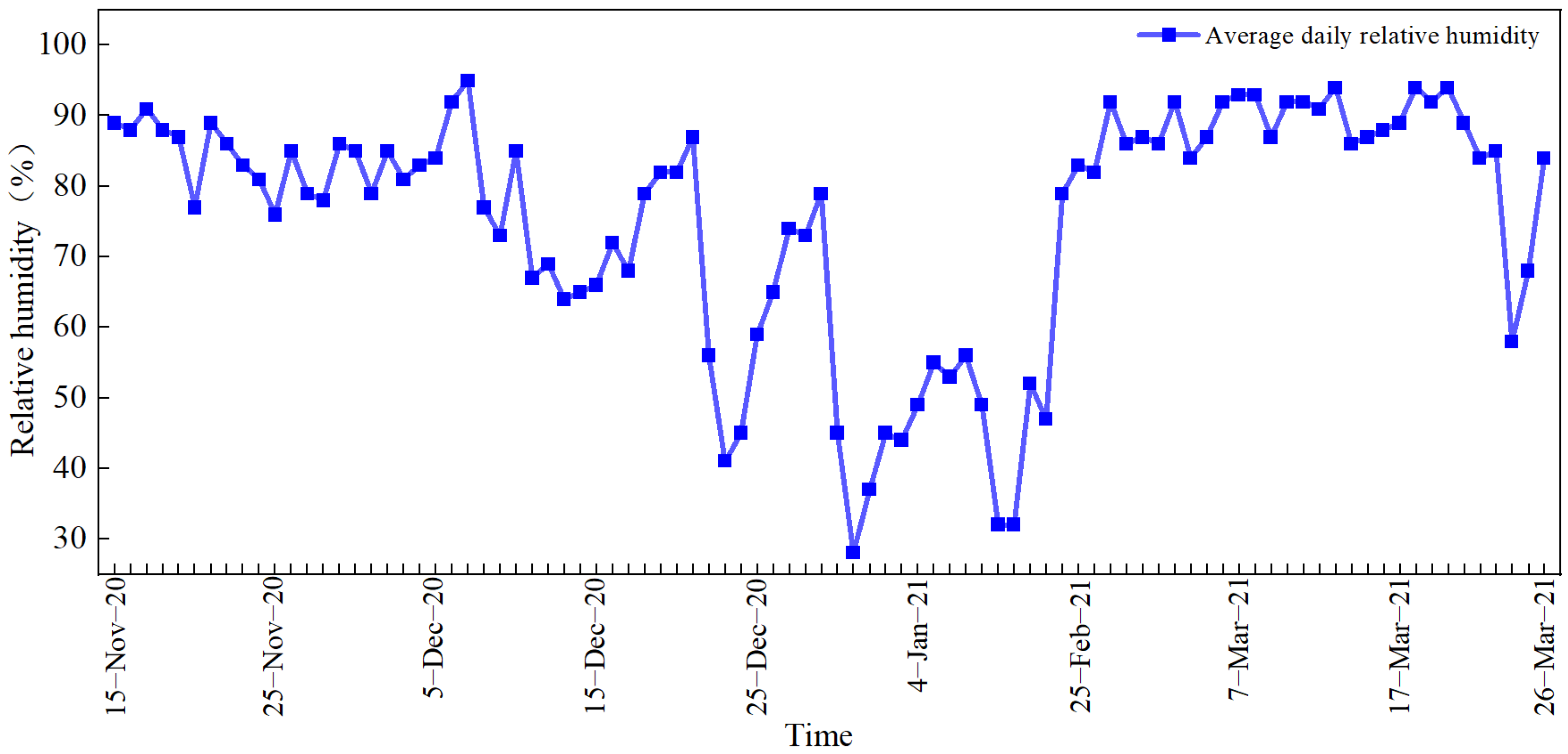
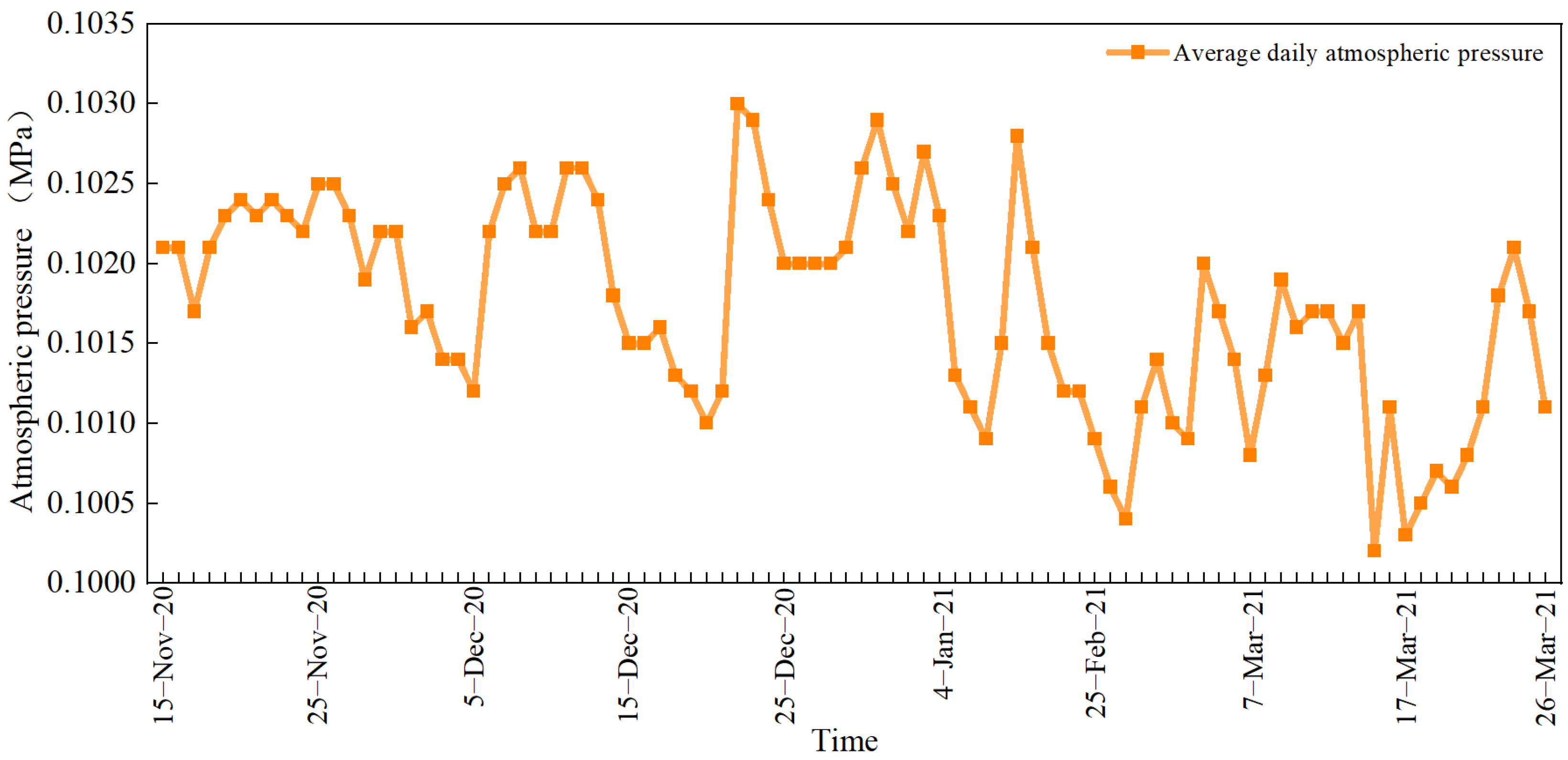
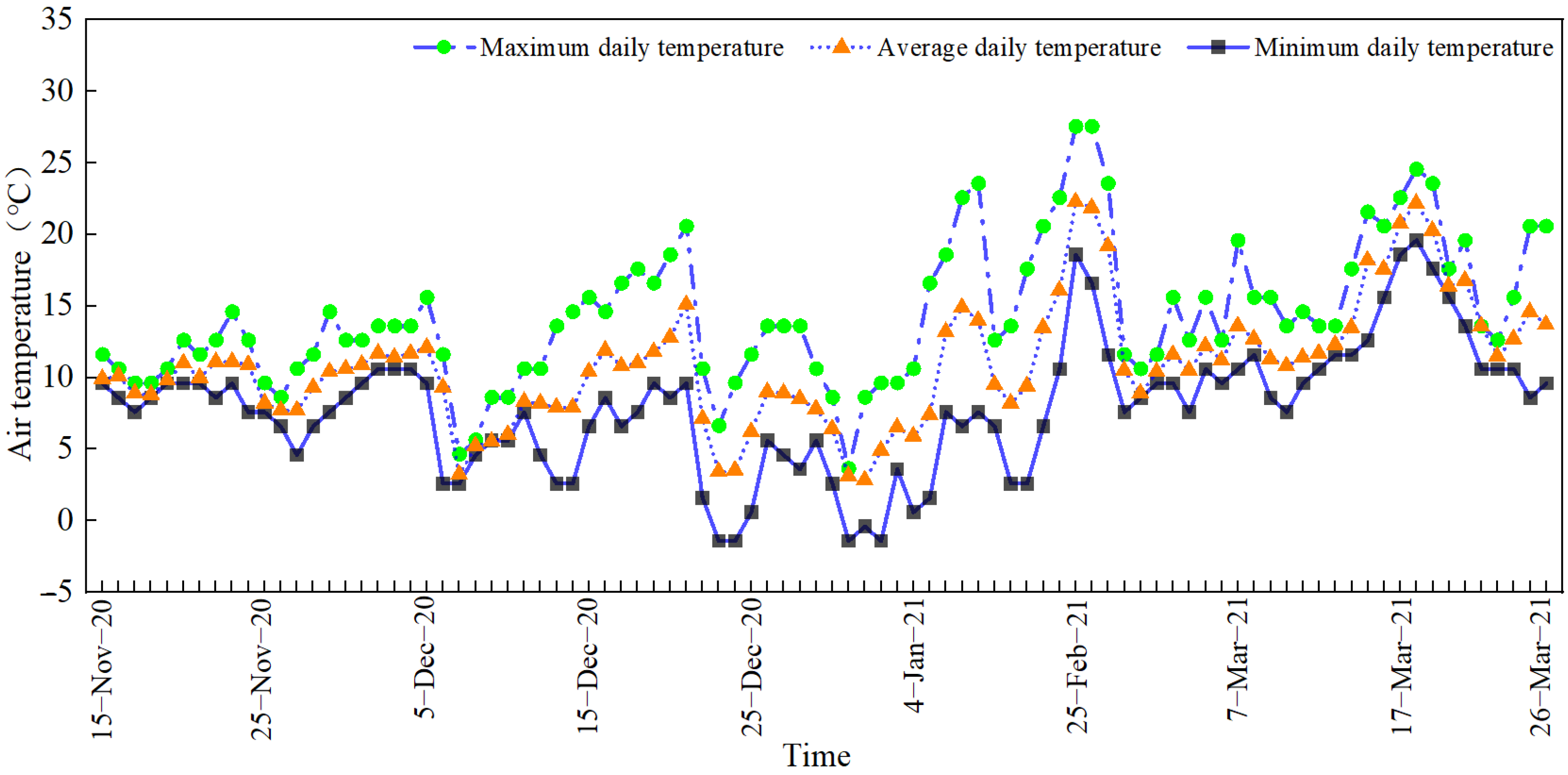
The experimental site was located in Changsha, Hunan Province, China. From June to September each year, ambient temperatures are relatively high, with greenhouse temperatures exceeding those of the external environment. Such conditions are unsuitable for coriander cultivation. Coriander is a cold-tolerant crop. Based on the selected variety and the local climate conducive to its growth, in this study, we scheduled the aeroponic water requirement experiments during winter and spring. An intelligent environmental parameter monitoring system was employed to collect meteorological data inside the greenhouse during the coriander experiments conducted from 22 November 2020 to 20 January 2021, and from 22 February 2021 to 23 March 2022—a total of 90 days. The main meteorological parameters included air temperature, relative humidity, atmospheric pressure, wind speed, radiation, and photoperiod. Daily air temperature data, shown in Figure 2. Analysis showed that during the trial, the maximum daily temperature reached 29.6 °C, the minimum dropped to −1.4 °C, and the mean daily temperature was 11.5 °C, indicating an overall temperature range suitable for coriander growth. Daily relative humidity data, shown in Figure 3, revealed a maximum of 95%, a minimum of 28%, and a mean of 77.7%. Daily atmospheric pressure data, shown in Figure 4, indicated a maximum of 0.103 MPa, a minimum of 0.1002 MPa, and a mean of 0.1017 MPa during the trial. Due to the semi-enclosed nature of the greenhouse, frequent ventilation was necessary, so internal wind speed was influenced by both external wind conditions and the operation of fans and ventilators.

2.6. Revised Formula for Crop Water Requirement Calculation

2.6.1. Calculation of Reference Crop Evapotranspiration

Reference crop evapotranspiration (ET₀), also known as reference crop transpiration, is the evaporation and transpiration rate from a hypothetical reference crop canopy. This metric is grounded in principles of energy balance and vapor diffusion, incorporating both crop physiological characteristics and the variation of aerodynamic parameters. The indicator offers a robust theoretical foundation and high computational precision [14,15]. Reference crop evapotranspiration serves as a comprehensive index for assessing the impact of various meteorological parameters on crop water requirements. The P-M formula is currently the most widely adopted approach for calculating reference ET₀. In 1998, the Food and Agriculture Organization (FAO) introduced the latest revision of the Penman equation, building on the 1977 version. This revised model has since seen broad adoption and has demonstrated high accuracy and applicability [16,17]. Based on the original P-M equation, the FAO P-M formula was derived to estimate reference crop evapotranspiration. The calculation formula is as follows:

$$E{T}_0={\displaystyle \frac{0.408\Delta (R_n-G)+\gamma \frac{900}{T+273}{U}_2(e_s-e_a)}{\Delta +\gamma (1+0.34U_2)}}$$

(1)

where ET₀ is the reference crop evapotranspiration, mm/d. ∆ is the slope of the saturation vapor pressure versus temperature relationship, kPa/°C. R_n is the net radiation, MJ/(m²/d). G is the soil heat fluxdensity, MJ/(m²/d). γ is the psychrometric constant, kPa/°C. T is the mean air temperature at 2 m above ground, °C. U₂ is the wind speed at a 2 m height, m/s. e_s is the saturation vapor pressure, kPa. e_a is the actual vapor pressure, kPa.

2.6.2. Revised P-M Formula for Crop Water Requirement Calculation

Owing to the semi-enclosed nature of greenhouse aeroponic cultivation systems, the internal environment is unique. Key microclimatic variables—air temperature, relative humidity, wind speed, atmospheric pressure, and radiation—differ substantially from those in open-field conditions. Outdoor wind speed exhibits continuous variation, whereas, without air circulation equipment, the wind speed inside a greenhouse approaches zero. When the internal wind speed of the greenhouse approaches zero, that is, U₂ = 0 in Equation (1), reference crop evapotranspiration is described by Equation (2):

$$E{T}_0={\displaystyle \frac{0.408\Delta (R_n-G)}{\Delta +\gamma }}$$

(2)

Equation (2) accounts only for the radiation component and omits aerodynamic terms, contradicting principles of vapor diffusion theory. To prevent the aerodynamic resistance term from becoming infinite when greenhouse wind speed is zero—thus yielding water requirement estimates inconsistent with field measurements—recent studies have introduced the aerodynamic resistance calculation as described in Equation (3) [18]:

$$r_a=4.72{\displaystyle \frac{{[\mathit{ln}(\frac{Z-d}{Z_0}\left)\right]}^2}{1+0.54U_2}}$$

(3)

where r_a is the aerodynamic resistance, s/m. Z is the wind speed measurement height, m. d is the zero plane displacement height, m. Z₀ is the surface roughness parameter, m.

Within the aeroponic cultivation greenhouse, under U₂ = 0 conditions, Equation (4) applies:

$$r_a=4.72{[\mathit{ln}({\displaystyle \frac{Z-d}{Z_0}}\left)\right]}^2$$

(4)

Based on recent literature [19], most crops can be reasonably approximated for Z₀ and d using the following empirical expressions:

$$Z_0=0.13h_c$$

(5)

$$d=0.64h_c$$

(6)

where h_c is the height of the coriander canopy, m.

Adjustments to aerodynamic modeling under zero wind speed conditions, as described by Liu [20] and Chen et al. [21], are referenced in this context. The resulting correction model for crop transpiration calculation is as follows:

$$E{T}_0={\displaystyle \frac{0.408\Delta (R_n-G)+\gamma \frac{1713(e_s-e_a)}{T+273}}{\Delta +1.64\gamma }}$$

(7)

2.6.3. Calculation of Crop Water Requirement

ET_c refers to the total amount of water lost through transpiration and evaporation during the entire growth period of crops under ideal conditions of adequate soil moisture, suitable fertility, and no pests or diseases, significant differences exist between the calculation of ET_c and ET₀. Owing to distinctions in ground cover, canopy characteristics, and aerodynamic resistance between crops and reference grass, the FAO has classified crop evapotranspiration estimation into two methodologies: the single crop coefficient approach and the dual crop coefficient approach. The equations for these methods are presented in Equation (8) [22,23,24]. In the crop coefficient method, the effects distinguishing field crops from grass are incorporated into the crop coefficient K_c, and ET_c is determined as the product of ET₀ and K_c. When applying the crop coefficient method to compute ET_c, it is generally understood to refer to field crops grown under optimal agronomic management and sufficient soil moisture conditions. Accurate estimation of crop evapotranspiration requires a comprehensive consideration of both soil evaporation and crop transpiration. The selection of an appropriate method should be guided by the purpose of the calculation, the required precision, and the availability of data.

$$E{T}_c=K_{c}E{T}_0$$

(8)

where ET_c is the crop evapotranspiration, in mm/d. K_c is the crop coefficient.

The crop coefficient varies by phenological stage, resulting in corresponding differences in water requirement across the crop lifecycle. The P-M equation defines reference crop evapotranspiration as the rate from a hypothetical reference crop canopy, where the assumed crop height is 0.12 m, with a fixed leaf surface resistance of 70 s·m⁻¹ and an albedo of 0.23. This is analogous to the evapotranspiration rate of a uniform, well-watered, actively growing green grass surface that fully covers the ground [25,26]. Drawing upon crop coefficient data for distinct growth stages as outlined in FAO Irrigation and Drainage Paper No. 56, and with reference to the works of Silva et al. [27] and Kumar et al. [28] on coriander crop coefficients, this study divides the coriander growth cycle into four phenological stages: initial stage (8 days), developmental stage (8 days), mid-stage (12 days), and late stage (4 days). Crop coefficients selected for each phase are as follows: K_c(ini) = 0.82, K_c(dev) = 1.03, K_c(mid) = 1.07, and K_c(late) = 0.93. The actual water requirement for coriander grown under greenhouse aeroponic conditions was determined in accordance with Equation (8).

2.7. Statistical Indicators

The statistical metrics include Root Mean Square Error (RMSE), Mean Absolute Error (MAE), Mean Absolute Percentage Error (MAPE), and the Coefficient of Determination (R²), which are used to evaluate the accuracy of different ET_c calculation models. The calculation formulas for the statistical metrics are as follows:

$$RMSE=\sqrt{{\displaystyle \frac{{{\sum }_{i=1}^n(x_i-y_i)}^2}{n}}}(0<RMSE<+\mathrm{\infty })$$

(9)

where n is the total number of samples. x_i(i = 1, 2, 3,…, n) is the predicted daily water requirement for coriander on day, mm·d⁻¹. y_i(i = 1, 2, 3,…, n) is the measured daily water consumption for coriander on day, mm·d⁻¹.

$$MAE={\displaystyle \frac{{\sum }_{i=1}^n|x_i-y_i|}{n}}(0<MAE<+\mathrm{\infty })$$

(10)

$$MAPE={\displaystyle \frac{{\sum }_{i=1}^n\left|\frac{x_i-y_i}{y_i}\right|}{n}}(0<MAPE<+\mathrm{\infty })$$

(11)

$$R^2=1-{\displaystyle \frac{{{\sum }_{i=1}^n(x_i-y_i)}^2}{{{\sum }_{i=1}^n(x_i-\overline{y_i})}^2}}(0<R^2<1)$$

(12)

where $\overline{y_i}$ is the mean value of the measured data.

3. Results

3.1. Calculation and Validation of Water Requirement for Crop Aeroponic Cultivation

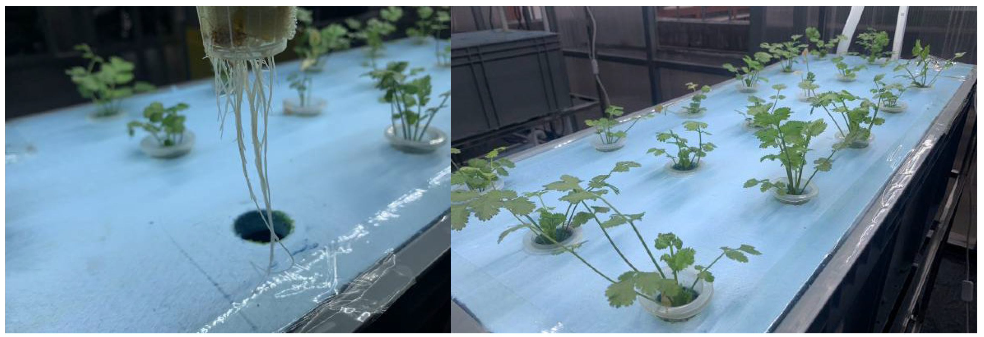
The daily evapotranspiration values of coriander, as well as the trends of daily crop evapotranspiration calculated using Equations (1), (7) and (8), are shown in Figure 5. From the figure, it is evident that the ET_c values calculated by both the P-M equation and the revised P-M equation exhibit irregular periodic variations over the time series. The maximum and minimum values recur periodically, while maintaining a consistent overall trend. The primary factors are the relative humidity and net radiation levels within the greenhouse atmosphere. Inadequate greenhouse ventilation results in water vapor accumulation and persistently elevated humidity levels, causing the actual vapor pressure to approach saturation and significantly reducing the vapor pressure deficit (VPD). Concurrently, the high-humidity environment induces stomatal closure in plants, suppressing transpiration, while restricted air movement impedes vapor diffusion. Collectively, these factors diminish evaporation efficiency. The daily evapotranspiration values calculated using the P-M equation were the highest, those determined by the revised P-M equation were intermediate, and the measured values were the lowest. As daily evapotranspiration increases, the error among daily evapotranspiration values calculated by the P-M equation, the revised P-M equation, and actual measurements becomes more pronounced. When daily evapotranspiration is relatively low, the results from these three approaches are closely aligned. During the second growth cycle, the maximum daily evapotranspiration for coriander, as observed from measured values, reached 4.792 mm/d. In the third growth cycle, the minimum daily evapotranspiration was 1.043 mm/d. The growth process of coriander aeroponic cultivation is shown in Figure 6.

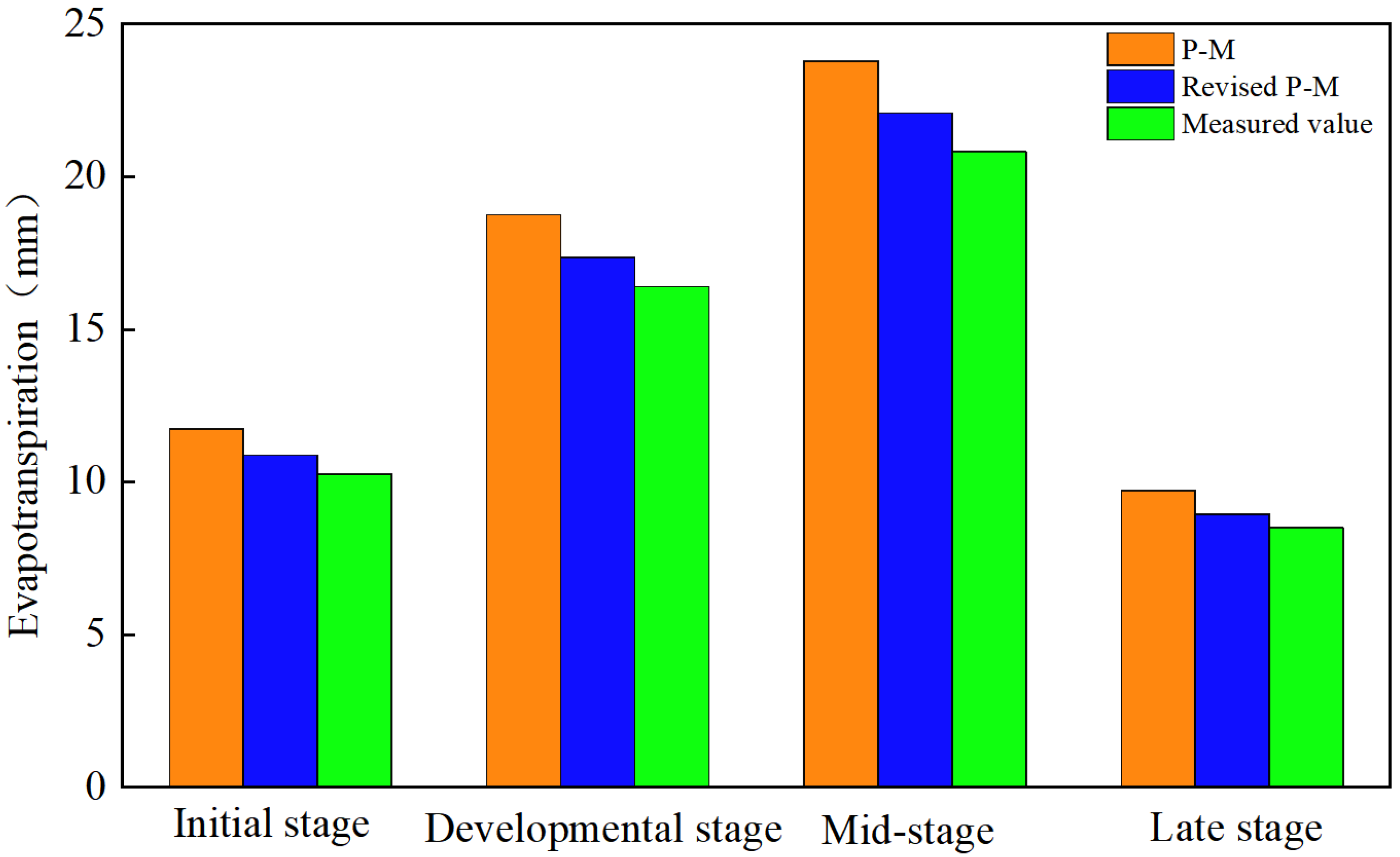
Utilizing measured values of daily crop evapotranspiration, the water requirements and calculated water requirements were analyzed according to four developmental stages of coriander growth: the initial stage, the developmental stage, the mid-stage, and the late stage. Figure 7 presents these results. Analysis reveals that, in the aeroponic cultivation of coriander, the water consumption during the mid-stage is greater than that during the developmental stage, which is in turn greater than mid-growth, followed by the initial stage. Variation in growth vigor across stages accounts for this phenomenon—coriander exhibits robust growth and heightened water requirement during the developmental stage and mid-stage, while growth and water use during the initial stage are comparatively lower. Further, the periods defined for the different growth stages are not uniform in duration; longer stages entail increased water requirement, while shorter stages result in lower requirement. The crop coefficient also plays a significant role. As the coriander progresses through its growth cycle, the crop coefficient is initially small, gradually increases, then tapers and stabilizes in the final stage, which drives differences in water requirement. For the P-M equation, the estimated water requirements are approximately 11.73 mm in the initial stage, 18.75 mm during the development stage, 23.79 mm in the mid-stage, and 9.72 mm in the late stage. By the revised P-M method, the estimated water requirement is roughly 10.87 mm in the initial stage, 17.37 mm during the development stage, 22.08 mm in the mid-stage, and 8.94 mm in the late stage. For actual measured values, water requirement is about 10.27 mm during the initial stage, 16.41 mm for the development stage, 20.82 mm in the mid-stage, and 8.5 mm during the late stage. The RMSE between the water requirement measured values and the calculated values using the P-M formula is 2.12 mm, the MAE is 2.0 mm, and the MAPE is 14.29%. The RMSE between the water requirement measured values and the calculated values using the revised P-M formula is 0.88 mm, the MAE is 0.82 mm, and the MAPE is 5.78%. The results indicate that the water requirement values calculated using the revised P-M formula are closer to the measured values.

3.2. Results and Analysis of Crop Water Requirement Prediction Model

3.2.1. Results and Analysis of the Random Forest Water Requirement Prediction Model

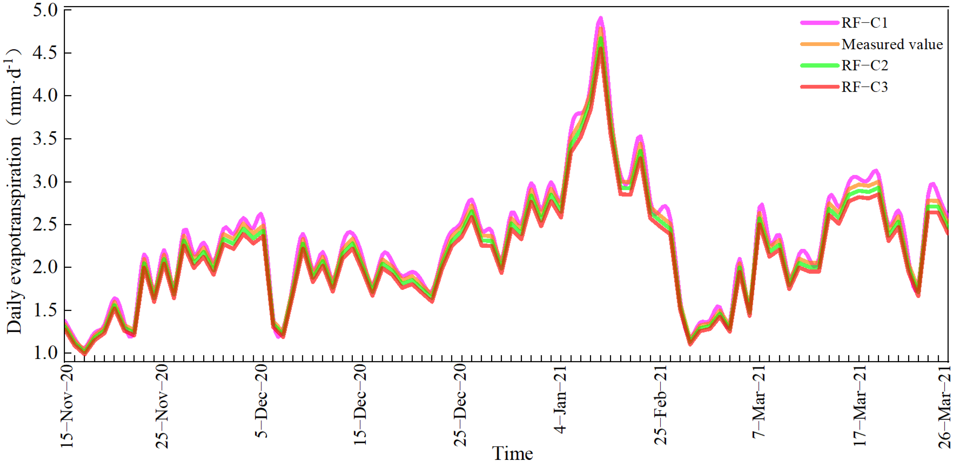
The Random Forest Algorithm refers to a classifier trained and predicted by aggregating results from multiple trees. Proposed initially by Leo Breiman, the Random Forest technique samples randomly from an original dataset to construct n distinct data subsets. Each subset is used to develop an independent decision tree model, and the final output is obtained either as the mean (in regression models) or the majority vote (in classification models) of all tree results [29,30]. For the aeroponic cultivation greenhouse scenario with coriander under study, the dataset included 90 real-time collected environmental parameter groups, such as air temperature, humidity, wind speed, atmospheric pressure, radiation, and photoperiod. The dataset was then split into two subsets: a training set and a test set. A randomization approach was employed to generate the training and test sets. The 90 groups of sample data were shuffled in temporal order, and 70 groups were randomly selected as the training set for the aeroponically grown coriander water requirement prediction model. The remaining 20 groups served as the test set for model evaluation. The meteorological data collected for the training set on a daily basis included such variables as air temperature, air humidity, wind speed, and atmospheric pressure, as well as radiation and photoperiod. The data were divided into three input configurations: C1 (air temperature, air humidity, wind speed and atmospheric pressure, radiation, and photoperiod), C2 (air temperature, air humidity, wind speed and atmospheric pressure, and photoperiod), and C3 (air temperature, air humidity). The RF model took C1, C2, and C3 as input features. The daily crop evapotranspiration, ET_c, of aeroponically cultivated coriander was set as the output variable. Comparisons between measured and predicted values were conducted. Figure 8 presents the comparison between the RF model water requirement prediction and the measured values.

RMSE, MAE, MAPE, and R² were used to assess the agreement between predicted and measured values of water requirement. After performing calculations and comparison, the RF model with C1 as input demonstrated the following statistics against measured coriander ET₀ in the test set: RMSE = 0.121 mm/d, MAE = 0.134 mm/d, MAPE = 2.123%, and R² = 0.971. With C2 as input, performance was RMSE = 0.147 mm/d, MAE = 0.261 mm/d, MAPE = 3.683%, and R² = 0.953. With C3 as input, statistics were RMSE = 0.172 mm/d, MAE = 0.298 mm/d, MAPE = 5.865%, and R² = 0.944. Feature indicators are listed in

Table 2. Comparison of RF model features with different input items.

Input Parameter	RMSE (mm/d)	MAE (mm/d)	MAPE (%)	R2
C1	0.121	0.134	2.123%	0.971
C2	0.147	0.261	3.683%	0.953
C3	0.172	0.298	5.865%	0.944

. Findings indicate that the coriander ET_c prediction model based on C1 inputs outperforms those based on C2 and C3 in terms of convergence speed, coefficient of determination, and overall performance. The RF model with C1 inputs yielded suspected values that most closely resembled measured values for ET₀ in aeroponically cultivated coriander.

3.2.2. Results and Analysis of the Biggang Water Requirement Prediction Model

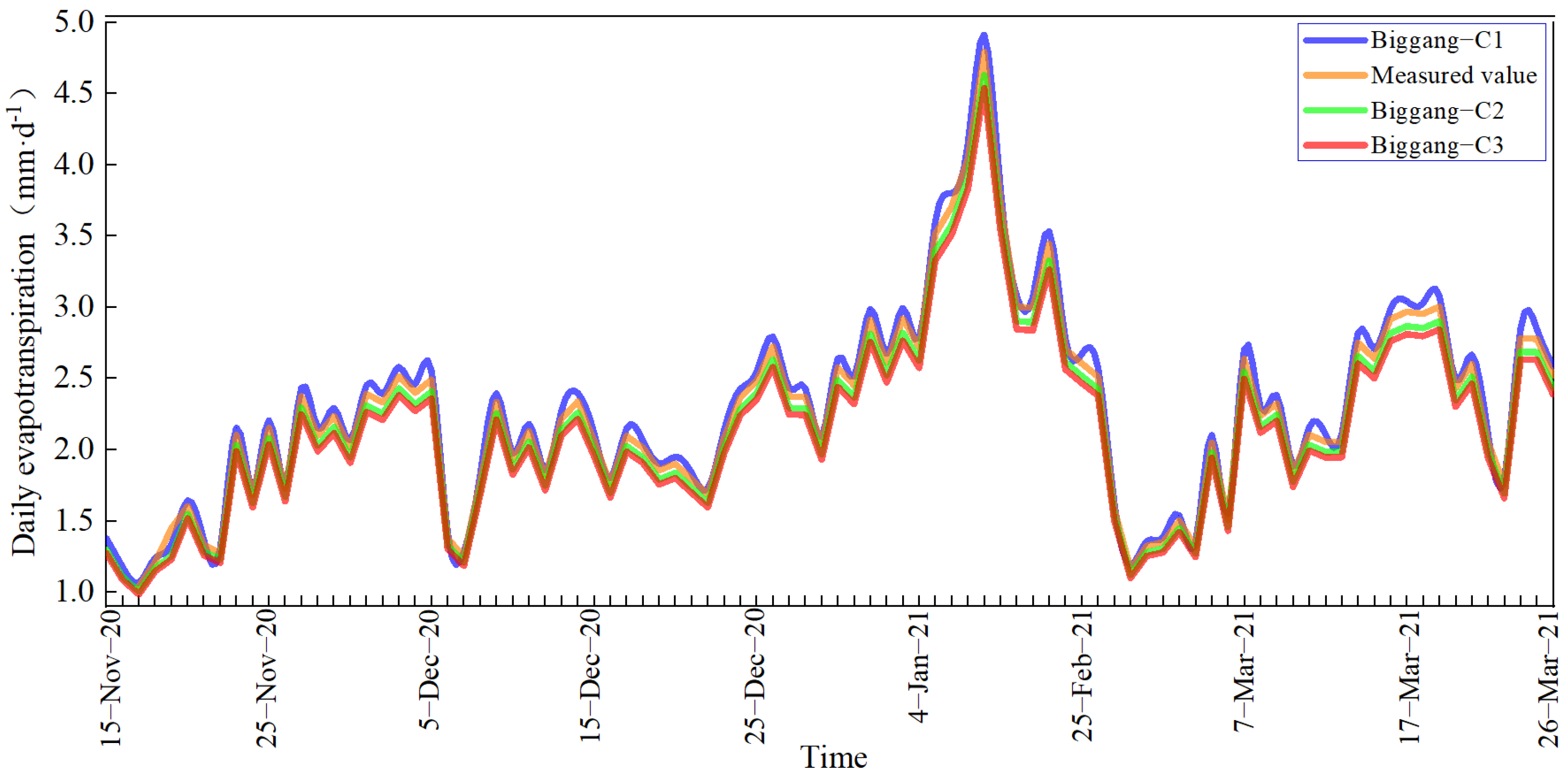
The Bagging algorithm, belonging to the ensemble learning methods in machine learning and recognized as one of the most popular collection models, was first proposed by Leo Breiman in 1996 [31,32]. The Bagging algorithm may be combined with other classification and regression methods to improve accuracy and stability, while reducing output variance and mitigating overfitting. In light of practical scenarios in aeroponic coriander cultivation greenhouses, the dataset consisted of 90 real-time samples of environmental parameters such as air temperature, air humidity, wind speed and atmospheric pressure, radiation, and photoperiod. The dataset was partitioned into two subsets: a training set and a test set. A randomization approach was utilized to generate both training and test sets. Ninety sets of sample data were randomly reordered by time sequence, after which seventy sets were selected as the training set for the aeroponic coriander water requirement prediction model, with the remaining twenty sets used as the test set for model evaluation. Collected as input features for the training set, daily meteorological variables primarily included air temperature, air humidity, wind speed and atmospheric pressure, radiation, and photoperiod. Divided into three input types, the dataset was organized as follows: C1 (air temperature, air humidity, wind speed and atmospheric pressure, radiation, and photoperiod), C2 (air temperature, air humidity, wind speed, atmospheric pressure, and photoperiod), and C3 (air temperature and air humidity). Employing the Random Forest model, C1, C2, and C3 were designated as input features for the predictive model. The daily reference crop evapotranspiration (ET₀) for aeroponic coriander cultivation was specified as the output variable, with measured and predicted values compared. Presented in Figure 9, a comparison between the predicted and measured water requirements from the Bagging model was conducted.

RMSE, MAE, MAPE, and R² were used to assess the agreement between predicted and measured values of water requirement. After calculation and comparison, results indicated that for the Bagging model with C1 inputs, measured ET₀ values for coriander showed RMSE = 0.132 mm/d, MAE = 0.148 mm/d, MAPE = 2.321%, and R² = 0.963 in the test set. With C2 inputs, RMSE = 0.176 mm/d, MAE = 0.269 mm/d, MAPE = 3.98%, and R² = 0.948. With C3 inputs, RMSE = 0.188 mm/d, MAE = 0.296 mm/d, MAPE = 5.932%, and R² = 0.939. Feature indicators are summarized in

Table 3. Comparison of Bagging model water requirement prediction and measured values.

Input Parameter	RMSE (mm/d)	MAE (mm/d)	MAPE (%)	R2
C1	0.132	0.148	2.321	0.963
C2	0.176	0.269	3.98%	0.948
C3	0.188	0.296	5.932%	0.939

. Indicated by the results, the crop ET₀ prediction model based on C1 inputs demonstrated superior convergence speed, coefficient of determination, and performance compared to those based on C2 and C3. The Bagging model using C1 inputs yielded ET₀ prediction values for aeroponic coriander that most closely matched measured values.

3.2.3. Results and Analysis of the M5P Tree Water Requirement Prediction Model

Defined as a binary decision tree, the M5P Model Tree Algorithm employs linear regression functions at the leaf (terminal) nodes, thereby supporting the prediction of continuous numerical attributes [33,34]. Providing a structural representation of data and piecewise linear fitting for classes, the model tree exhibits a conventional decision tree structure. Classification can be achieved by employing a standard method that transforms the classification task into a function optimization problem. Compared to traditional linear regression, the M5P model tree offers greater accuracy for predicting nonlinear data, and its rules and regression models are easy to interpret. According to the practical conditions of aeroponic coriander cultivation in the greenhouse, a dataset consisting of 90 real-time samples of environmental parameters—air temperature, air humidity, wind speed, atmospheric pressure, radiation, and photoperiod—was collected. The dataset was partitioned into two subsets: a training set and a test set. By employing a randomized procedure, the 90 sets of sample data were temporally shuffled, with 70 groups randomly selected as the training set for the water requirement prediction model of aeroponic cultivation of coriander, while the remaining 20 groups comprised the test set. Collected as inputs for the training set, daily meteorological data primarily included air temperature, air humidity, wind speed, atmospheric pressure, radiation, and photoperiod. Three types of input variables were defined for modeling: C1 (air temperature, air humidity, wind speed, atmospheric pressure, radiation, and photoperiod), C2 (air temperature, air humidity, wind speed, atmospheric pressure, and photoperiod), and C3 (air temperature and air humidity). Using the M5P model tree, C1, C2, and C3 were set as input features for the predictive model, with daily reference crop evapotranspiration (ET₀) for aeroponic cultivation of coriander as the output variable. Comparisons were performed between observed and predicted values. A comparison of the predicted and measured water requirements using the M5P model tree is presented in Figure 10.

RMSE, MAE, MAPE, and R² were used to assess the agreement between predicted and measured values of water requirement. Through data analysis and comparison, it was found that, with C1 as input, the M5P model tree achieved RMSE = 0.1462 mm/d, MAE = 0.187 mm/d, MAPE = 2.403%, and R² = 0.961; with C2, RMSE = 0.201 mm/d, MAE = 0.284 mm/d, MAPE = 4.21%, and R² = 0.946; with C3 (for the Bagging model), RMSE = 0.216 mm/d, MAE = 0.366 mm/d, MAPE = 5.986%, and R² = 0.928. Feature indicators are presented in

Table 4. Comparison of M5P model features with different input items.

Input Parameter	RMSE (mm/d)	MAE (mm/d)	MAPE (%)	R2
C1	0.1462	0.187	2.403%	0.961
C2	0.201	0.284	4.21%	0.946
C3	0.216	0.366	5.986%	0.928

. Results indicate that, with C1 as input, the ET₀ prediction model converges faster and performs better in terms of determination coefficient and accuracy compared to the C2 and C3 models. The Bagging model with C1 inputs yielded ET₀ predictions for aeroponic cultivation of coriander that were more closely aligned with measured values.

4. Discussion

Aeroponic cultivation in greenhouses operates in a relatively enclosed environment characterized by limited light exposure, high controllability of temperature and humidity, and low wind speed. Unlike traditional soil-based cultivation, which relies on natural precipitation, this system depends entirely on artificially formulated nutrient solutions for water supply [35]. Compared to conventional methods, this method enables precise recording of water consumption throughout the entire growth cycle of crops, providing a robust data foundation for studying crop water requirements under varying environmental conditions [36]. Currently, systematic theories and methods for calculating and predicting water requirements in aeroponic cultivation systems are still lacking, and related research remains in its preliminary stages. As agricultural production shifts toward precision practices that emphasize quality, efficiency, resource conservation, and environmental sustainability, it is imperative to systematically investigate the dynamics of greenhouse environmental factors and their relationship with water requirement in aeroponic cultivation. Such research holds significant scientific importance for achieving precise irrigation, improving crop yield and quality, and promoting the sustainable development of modern agriculture.

This study employed aeroponic cultivation technology with coriander as the test crop. The crop water requirement was estimated using both the FAO56 P-M equation and a revised FAO56 P-M equation. When compared to measured water requirements, the RMSE between the water requirement measured values and the calculated values using the P-M formula is 2.12 mm, the MAE is 2.0 mm, and the MAPE is 14.29%. The RMSE between the water requirement measured values and the calculated values using the revised P-M formula is 0.88 mm, the MAE is 0.82 mm, and the MAPE is 5.78%. The results indicate that the water requirement values calculated using the revised P-M formula are closer to the measured values. By referencing coriander evapotranspiration, this study utilized the RF, Bagging, and M5P algorithms. The major environmental factors affecting crop water requirements were selected as input features, with the daily reference crop water requirement as the output variable. Models for predicting the water requirement of coriander were subsequently developed. A comparison of different input features for the RF, Bagging, and M5P models is provided in Table 2, Table 3 and Table 4. The results demonstrate that, with C1 (air temperature, relative humidity, atmospheric pressure, wind speed, radiation, and photoperiod) as input features, the RF model achieved faster convergence, a higher determination coefficient, and better performance than RF-C2, RF-C3, Bagging-C1, Bagging-C2, Bagging-C3, M5P-C1, M5P-C2, and M5P-C3 models for predicting the water requirement of coriander. High predictive accuracy and adaptability were obtained, making the proposed approach more suitable for estimating the water requirements of aeroponic cultivation of coriander. The findings may provide theoretical guidance for establishing efficient, intelligent, and water-saving cultivation and irrigation strategies in aeroponic cultivation crop production.

The methodology developed in this study, which combines a revised FAO56 P-M equation with machine learning algorithms to predict water requirements for coriander aeroponic cultivation, demonstrates certain innovations compared to recent related research. The direct application of the traditional FAO56 P-M formula in non-standard environments exhibits significant deviations, a finding consistent with our conclusion that the unique water requirement mechanisms in aeroponic cultivation systems render conventional models inadequate [37,38]. However, modification strategies vary across different regions and environmental conditions. For instance, Júnior et al. [39] estimated reference evapotranspiration for the Brazilian savanna (Cerrado) region in the absence of complete meteorological data. The results showed that radiation data had the highest impact on ET₀ in the local study area and in regions with similar climatic conditions. Furthermore, when radiation data were missing, the FAO radiation estimation procedure was not applicable. Sharafi et al. [40] calibrated 32 empirical equations for estimating ET₀ in different climatic regions of Iran. The results demonstrated that the calibrated equations achieved average R² = 0.73, 0.67, and 0.78; RMSE = 35.14, 35.02, and 30.20 mm/year; and MBE = −5.6, −3.89, and 2.57 mm/year, respectively. The use of calibrated empirical equations provides a more accurate estimation of ET₀. Therefore, the universality of the FAO56-PM model is still limited by specific crop varieties, greenhouse facilities, and regional climatic conditions, and its promotion requires recalibration and verification.

This study employs a combined approach of multi-indicator validation and multi-model comparison, incorporating statistical metrics such as RMSE, MAE, MAPE, and R² to evaluate the discrepancy between predicted and observed values, thereby enhancing the reliability of the results. This methodology aligns with the approach used by Dong et al. [41], who assessed the accuracy of different machine learning models using statistical metrics such as MAE, RMSE, and R². By setting different combinations of climate data inputs, the performance of various machine learning models, such as RF, Bagging, and M5P, was compared, and model selection was implemented. This approach is similar to the method used by Mokhtar et al. [42] to predict irrigation water demand using different models. Ultimately, the RF model performed optimally under C1 input conditions, and its high-precision characteristics align with the robust performance of RF in existing agricultural research.

5. Conclusions

The results show that the RF-C1 prediction model demonstrates reductions in RMSE, MAE, and MAPE of 0.026, 0.127, and 1.56%, respectively, compared to the RF-C2 model, with an increase in R² of 0.018. The RF-C1 model outperforms the RF-C3 model with decreases in RMSE, MAE, and MAPE by 0.051, 0.164, and 3.74%, and an increase in R² of 0.0274. Compared to the Bagging-C1 model, the RF-C1 model achieves reductions in RMSE, MAE, and MAPE by 0.011, 0.014, and 0.2%, while R² increases by 0.008. The RF-C1 model surpasses the Bagging-C2 model with decreases in RMSE, MAE, and MAPE of 0.055, 0.135, and 1.86%, and an increase in R² of 0.023. When compared to the Bagging-C3 model, the RF-C1 model exhibits reductions in RMSE, MAE, and MAPE of 0.067, 0.167, and 3.81%, with R² increasing by 0.032. Utilizing C1 as input, the RF model for coriander ET₀ prediction delivers superior convergence speed, determination coefficient, and performance relative to RF-C2, RF-C3, Bagging-C1, Bagging-C2, Bagging-C3, M5P-C1, M5P-C2, and M5P-C3 models for crop water requirement forecasting. It is more suitable for predicting the water requirements of coriander aeroponic cultivation and can provide a theoretical reference for the establishment of efficient and intelligent water-saving cultivation and irrigation systems for crop aeroponic cultivation.

This study can be applied to Controlled Environment Agriculture (CEA) in the future by deploying a multi-source sensor network to collect real-time environmental parameter data. This will facilitate the establishment of adaptive water requirement patterns for greenhouse crops and enable the training of dynamic machine learning models. The optimized model will be embedded into the central control system of CEA, allowing coordinated adjustment of aeroponic cultivation equipment and spray duration. Such an integrated approach will realize a water-saving optimization system characterized by “environmental perception, model-based decision-making, and precise execution.” This framework can provide low-consumption and high-efficiency irrigation decision support for greenhouses, plant factories, and other facility-based agricultural systems.

References

1. Luo, W.; Chen, M.; Kang, Y.; Li, W.; Li, D.; Cui, Y.; Shahbaz, K.; Luo, Y. Analysis of Crop Water Requirements and Irrigation Demands for Rice: Implications for Increasing Effective Rainfall. Agric. Water Manag. 2022, 260, 107285. [Google Scholar] [CrossRef]
2. Agrawal, A.; Srivastava, P.; Tripathi, V.; Maurya, S.; Sharma, R.; Shrinivasa, D.J. Future Projections of Crop Water and Irrigation Water Requirements Using a Bias-Corrected Regional Climate Model Coupled with CROPWAT. J. Water Clim. Change 2023, 14, 1147–1161. [Google Scholar] [CrossRef]
3. Bwambale, E.; Abagale, F.; Anornu, G. Smart Irrigation Monitoring and Control Strategies for Improving Water Use Efficiency in Precision Agriculture: A Review. Agric. Water Manag. 2022, 260, 107324. [Google Scholar] [CrossRef]
4. Huang, Y.; Zhong, X.; Gong, D.; Huo, Z. The Optimization of Agricultural Irrigation Based on Big Data: An Integrated Analysis of Climate Conditions, Water Resources, Soil Types, and Crop Demand. Adv. Resour. Res. 2025, 5, 386–413. [Google Scholar]
5. Gaznayee, H.A.A.; Zaki, S.H.; Al-Quraishi, A.M.F.; Aliehsan, P.H.; Hakzi, K.K.; Razvanchy, H.A.S.; Riksen, M.; Mahdi, K. Integrating Remote Sensing Techniques and Meteorological Data to Assess the Ideal Irrigation System Performance Scenarios for Improving Crop Productivity. Water 2023, 15, 1605. [Google Scholar] [CrossRef]
6. Ju, X.; Lei, T.; Guo, X.; Sun, X.; Ma, J.; Liu, R.; Zhang, M. Evaluation of Suitable Water–Zeolite Coupling Regulation Strategy of Tomatoes with Alternate Drip Irrigation Under Mulch. Horticulturae 2022, 8, 536. [Google Scholar] [CrossRef]
7. Lakhiar, I.A.; Gao, J.; Syed, T.N.; Chandio, F.A.; Tunio, M.H.; Ahmad, F.; Solangi, K.A. Overview of the Aeroponic Agriculture–an Emerging Technology for Global Food Security. Int. J. Agric. Biol. Eng. 2020, 13, 1–10. [Google Scholar] [CrossRef]
8. Garzón, J.; Montes, L.; Garzón, J.; Lampropoulos, G. Systematic Review of Technology in Aeroponics: Introducing the Technology Adoption and Integration in Sustainable Agriculture Model. Agronomy 2023, 13, 2517. [Google Scholar] [CrossRef]
9. Qureshi, W.A.; Gao, J.; Elsherbiny, O.; Mosha, A.H.; Tunio, M.H.; Qureshi, J.A. Boosting Aeroponic System Development with Plasma and High-Efficiency Tools: Ai and Iot—A Review. Agronomy 2025, 15, 546. [Google Scholar] [CrossRef]
10. Eldridge, B.M.; Manzoni, L.R.; Graham, C.A.; Rodgers, B.; Farmer, J.R.; Dodd, A.N. Getting to the Roots of Aeroponic Indoor Farming. New Phytol. 2020, 228, 1183–1192. [Google Scholar] [CrossRef]
11. Fasciolo, B.; Awouda, A.; Bruno, G.; Lombardi, F. A Smart Aeroponic System for Sustainable Indoor Farming. Procedia CIRP 2023, 116, 636–641. [Google Scholar] [CrossRef]
12. Liu, S.; Qiang, X.; Liu, H.; Han, Q.; Yi, P.; Ning, H.; Li, H.; Wang, C.; Zhang, X. Effects of Nutrient Solution Application Rates on Yield, Quality, and Water–Fertilizer Use Efficiency on Greenhouse Tomatoes Using Grown-in Coir. Plants 2024, 13, 893. [Google Scholar] [CrossRef] [PubMed]
13. Qu, F.; Zhang, J.; Wang, J.; Ma, X.; Gao, Z.; Liu, D.; Hu, X. Genetic Algorithm-Based Optimization of Nutrient Solution Formula for Substrate-Cultivated Cucumber. Trans. Chin. Soc. Agric. Eng. 2021, 37, 96–104. [Google Scholar]
14. Pimentel, R.; Arheimer, B.; Crochemore, L.; Andersson, J.C.M.; Pechlivanidis, I.G.; Gustafsson, D. Which Potential Evapotranspiration Formula to Use in Hydrological Modeling World-Wide? Water Resour. Res. 2023, 59, e2022WR033447. [Google Scholar] [CrossRef]
15. Pereira, L.S.; Paredes, P.; Oliveira, C.M.; Montoya, F.; López-Urrea, R.; Salman, M. Single and Basal Crop Coefficients for Estimation of Water Use of Tree and Vine Woody Crops with Consideration of Fraction of Ground Cover, Height, and Training System for Mediterranean and Warm Temperate Fruit and Leaf Crops. Irrig. Sci. 2024, 42, 1019–1058. [Google Scholar] [CrossRef]
16. Song, N.; Sun, J.; Wang, J.; Chen, Z.; Qiang, X.; Liu, Z. Analysis of Difference in Crop Coefficients Based on Modified Penman and Penman-Monteith Equations. Trans. Chin. Soc. Agric. Eng. 2013, 29, 88–97. [Google Scholar]
17. Matsui, H.; Osawa, K. Alternative Net Longwave Radiation Equation for the Fao Penman–Monteith Evapotranspiration Equation and the Penman Evaporation Equation. Theor. Appl. Climatol. 2023, 153, 1355–1360. [Google Scholar] [CrossRef]
18. Al-Dughairi, A.B.A.; Bourouba, M.F. Calibration of Two Models for Estimating Reference Evapotranspiration by Using Fao-56 Penman-Monteith Model under Arid Conditions. Eng. Herit. J. 2023, 7, 113–121. [Google Scholar] [CrossRef]
19. Valiantzas, J.D. Simplified Forms for the Standardized FAO-56 Penman–Monteith Reference Evapotranspiration Using Limited Weather Data. J. Hydrol. 2013, 505, 13–23. [Google Scholar] [CrossRef]
20. Liu, H. Water Requirement and Optimal Irrigation Index for Effective Water Use and High-Quality of Tomato in Greenhouse. Ph.D. Thesis, Chinese Academy of Agricultural Sciences, Beijing, China, 2010. [Google Scholar]
21. Chen, X.; Cai, H.; Li, H.; Wang, J.; Du, W. Calculation of Crop Evapotranspiration in Greenhouse. J. Appl. Ecol. 2007, 18, 317–321. [Google Scholar]
22. Allen, R.G.; Pereira, L.S.; Raes, D.; Smith, M. Crop Evapotranspiration-Guideline for Computing Crop Water Requirements. Irrig. Drain. 1998, 56, 300. [Google Scholar]
23. Allen, R.G.; Kilic, A.; Robison, C.W. Current Frameworks for Reference ET and Crop Coefficient Calculation. In Proceedings of the 6th Decennial National Irrigation Symposium, San Diego, CA, USA, 6–8 December 2021; American Society of Agricultural and Biological Engineers: St Joseph, MI, USA, 2021. [Google Scholar]
24. Chatterjee, S.; Stoy, P.C.; Debnath, M.; Nayak, A.K.; Swain, C.K.; Tripathi, R.; Chatterjee, D.; Mahapatra, S.S.; Talib, A.; Pathak, H. Actual Evapotranspiration and Crop Coefficients for Tropical Lowland Rice (Oryza sativa L.) in Eastern India. Theor. Appl. Climatol. 2021, 146, 155–171. [Google Scholar] [CrossRef]
25. Solangi, G.S.; Shah, S.A.; Alharbi, R.S.; Panhwar, S.; Keerio, H.A.; Kim, T.W.; Memon, J.A.; Bughio, A.D. Investigation of Irrigation Water Requirements for Major Crops Using Cropwat Model Based on Climate Data. Water 2022, 14, 2578. [Google Scholar] [CrossRef]
26. Ezenne, G.I.; Eyibio, N.U.; Tanner, J.L.; Asoiro, F.U.; Obalum, S.E. An Overview of Uncertainties in Evapotranspiration Estimation Techniques. J. Agrometeorol. 2023, 25, 173–182. [Google Scholar] [CrossRef]
27. Silva, V.D.P.D.; de Sousa, I.F.; Tavares, A.L.; Silva, T.G.F.D.; Silva, M.T. Evapotranspiration, Crop Coefficient and Water Use Efficiency of Coriander Grown in Tropical Environment. Hortic. Bras. 2018, 36, 446–452. [Google Scholar] [CrossRef]
28. Kumar, D.; Rank, P.H. Estimation of Crop Evapotranspiration and Crop Coefficient for Coriander Using Portable Automatic Closed Canopy Chamber. J. Agrometeorol. 2023, 25, 547–552. [Google Scholar] [CrossRef]
29. Majumdar, P.; Bhattacharya, D.; Mitra, S.; Solgi, R.; Oliva, D.; Bhusan, B. Demand Prediction of Rice Growth Stage-Wise Irrigation Water Requirement and Fertilizer Using Bayesian Genetic Algorithm and Random Forest for Yield Enhancement. Paddy Water Environ. 2023, 21, 275–293. [Google Scholar] [CrossRef]
30. Saggi, M.K.; Jain, S. Application of Fuzzy-Genetic and Regularization Random Forest (Fg-Rrf): Estimation of Crop Evapotranspiration (ETc) for Maize and Wheat Crops. Agric. Water Manag. 2020, 229, 105907. [Google Scholar] [CrossRef]
31. TR, J.; Reddy, N.V.S.; Acharya, U.D. Modeling Daily Reference Evapotranspiration From Climate Variables: Assessment of Bagging and Boosting Regression Approaches. Water Resour. Manag. 2023, 37, 1013–1032. [Google Scholar] [CrossRef]
32. Salam, R.; Islam, A.R.M.T. Potential of Rt, Bagging and Rs Ensemble Learning Algorithms for Reference Evapotranspiration Prediction Using Climatic Data-Limited Humid Region in Bangladesh. J. Hydrol. 2020, 590, 125241. [Google Scholar] [CrossRef]
33. Samadianfard, S.; Rousta, Z.; Sharafi, M. Prediction of Daily Reference Evapotranspiration with M5P, Gaussian Process Regression and Support Vector Regression Methods. Water Soil Sci. 2024, 34, 156–176. [Google Scholar]
34. Sharafi, M.; Abdi, E.; Mohebbiyan, M.; Samadianfard, S. Prediction of Daily Evapotranspiration Using the Strategy of Combining Tree Models with Empirical Hargreaves Method. Water Soil Sci. 2024, 34, 107–119. [Google Scholar]
35. Shamshiri, R.R.; Jones, J.W.; Thorp, K.R.; Ahmad, D.; Man, H.C.; Taheri, S. Review of Optimum Temperature, Humidity, and Vapour Pressure Deficit for Microclimate Evaluation and Control in Greenhouse Cultivation Of Tomato: A Review. Int. Agrophysics 2018, 32, 287–302. [Google Scholar] [CrossRef]
36. Peng, Y.; Xiao, Y.; Fu, Z.; Dong, Y.; Zheng, Y.; Yan, H.; Li, X. Precision Irrigation Perspectives on the Sustainable Water-Saving of Field Crop Production in China: Water Demand Prediction and Irrigation Scheme Optimization. J. Clean. Prod. 2019, 230, 365–377. [Google Scholar] [CrossRef]
37. Didari, S.; Ahmadi, S.H. Calibration and Evaluation of the FAO56-Penman-Monteith, FAO24-Radiation, and Priestly-Taylor Reference Evapotranspiration Models Using the Spatially Measured Solar Radiation Across a Large Arid and Semi-Arid Area in Southern Iran. Theor. Appl. Climatol. 2019, 136, 441–455. [Google Scholar] [CrossRef]
38. Tomar, A.S. Evaluating the Performance of Calibrated Temperature-Based Equations as Compared to Standard Fao-56 Penman Monteith Equation in Humid Climatic Condition of Dehradun (India). J. Agric. Eng. 2022, 59, 386–403. [Google Scholar] [CrossRef]
39. Júnior, L.C.G.D.V.; Vourlitis, G.L.; Curado, L.F.A.; Palácios, R.D.S.; Nogueira, J.D.S.; Lobo, F.D.A.; Islam, A.R.M.T.; Rodrigues, T.R. Evaluation of FAO-56 Procedures for Estimating Reference Evapotranspiration Using Missing Climatic Data for a Brazilian Tropical Savanna. Water 2021, 13, 1763. [Google Scholar] [CrossRef]
40. Sharafi, S.; Ghaleni, M.M. Calibration of Empirical Equations for Estimating Reference Evapotranspiration in Different Climates of Iran. Theor. Appl. Climatol. 2021, 145, 925–939. [Google Scholar] [CrossRef]
41. Dong, S.; Ma, Q.; Yu, C.; Li, L.; Liu, H.; Cui, G.; Qiu, H.; Yang, S.; Wang, G. Comparative Analysis of Crop Coefficient Approaches and Machine Learning Models for Predicting Water Requirements in Three Major Crops in Coastal Saline-Alkali Land. Agronomy 2025, 15, 492. [Google Scholar] [CrossRef]
42. Mokhtar, A.; Al-Ansari, N.; El-Ssawy, W.; Graf, R.; Aghelpour, P.; He, H.; Hafe, S.M.; Abuarab, M. Prediction of Irrigation Water Requirements for Green Beans-Based Machine Learning Algorithm Models in Arid Region. Water Resour. Manag. 2023, 37, 1557–1580. [Google Scholar] [CrossRef]
Figure 1. Composition of greenhouse crop aeroponic cultivation system. Note: 1. Air circulation exhaust fan. 2. Shade net. 3. Multi-layer aeroponics cultivation device. 4. Aeroponic crops. 5. Plant growth LED lights. 6. Galvanized sheet. 7. Environmental monitoring system. 8. Wet curtain–fan system. 9. Water storage tank. 10. Nutrient solution storage tank. 11. Nutrient solution supply pipe. 12. Atomizing nozzle. 13. Nutrient solution return pipe. 14. Cultivation container. 15. Nutrient solution mixing equipment. 16. Fertilizer barrel. 17. Electrical cabinet.
Horticulturae 11 01034 g001
Figure 2. 90-day daily air temperature data in aeroponic cultivation greenhouse.
Horticulturae 11 01034 g002
Figure 3. 90-day daily humidity data in aeroponic cultivation greenhouse.
Horticulturae 11 01034 g003
Figure 4. 90-day daily atmospheric pressure data in aeroponic cultivation greenhouse.
Horticulturae 11 01034 g004
Figure 5. Single coriander plant water requirement measured and calculated value changes at different growth cycles.
Horticulturae 11 01034 g005
Figure 6. Diagram of the growth process of coriander aeroponic cultivation.
Horticulturae 11 01034 g006
Figure 7. Single coriander plant aeroponic cultivation evapotranspiration measured and calculated values in four different growth periods.
Horticulturae 11 01034 g007
Figure 8. Comparison of RF model water requirement prediction and measured values.
Horticulturae 11 01034 g008
Figure 9. Comparison of Bagging model water requirement prediction and measured values.
Horticulturae 11 01034 g009
Figure 10. Comparison of M5P model water requirement prediction and measured values.
Horticulturae 11 01034 g010