Using Calibration Transfer Strategy to Update Hyperspectral Model for Quantitating Soluble Solid Content of Blueberry Across Different Batches

Abstract

Model updating is a challenging task with regard to maintaining the performance of non-destructive detection models while using hyperspectral imaging techniques for detecting the internal quality of fresh fruits like blueberries. Different sample batches and differences in hyperspectral image acquisition environments may lead to a significant decline in the performance of hyperspectral detection models. This study investigated the transferability of a hyperspectral model for the quantitating soluble solid content of blueberries across different batches for two harvest years. Hyperspectral images and SSC values of blueberries were collected from two batches, including 364 samples from 2024 and 175 samples from 2025. The differences between SSC measurements and spectral data across these two batches were analyzed. Based on the sample dataset of the year 2024, a high-performance quantitative model for detecting SSC values was established by combining it with partial least squares regression (PLSR) and competitive adaptive reweighted sampling (CARS). This high-performance model could achieve a high determination coefficient (${\mathrm{R}}_{\mathrm{P}}^2$) of 0.8965 and a low root mean square error of prediction (RMSEP) of 0.3707 °Brix. Using the sample dataset for the year 2025, the hyperspectral model was updated by the semi-supervised parameter-free calibration enhancement (SS-PFCE) algorithm. The updated model performed better than those established using individual datasets from 2024 and 2025, and obtained an ${\mathrm{R}}_{\mathrm{P}}^2$ of 0.8347 and an RMSEP of 0.4930 °Brix. This indicates that the calibration transfer strategy is superior in improving hyperspectral model performance. This study demonstrated that the SS-PFCE algorithm, as a calibration transfer strategy, could effectively improve the transferability of the established model for detecting the SSC of blueberries across different sample batches.

1. Introduction

The blueberry, a small berry-producing shrub from the Ericaceae family and the genus Vaccinium, has a unique flavor that makes it popular in the fresh fruit market and is also widely used in food processing. Blueberries are rich in anthocyanins, vitamin C, fiber, and various antioxidants, making them an important ingredient in the development of functional foods and health products [1,2,3]. In food processing, blueberries can be made into juice, jam, wine, and dried fruit, as well as blueberry-flavored candy, yogurt, beverages, and other products [4,5]. The natural pigments in blueberries (mainly anthocyanins) are also used as food colorants, which are favored for their health benefits and safety [6]. The soluble solid content (SSC) is a key factor in determining the taste, maturity, and quality of blueberries. Traditional methods for detecting SSC, such as digital refractometers, rely on destructive sampling and chemical analysis, which are time-consuming and irreversible, making them unsuitable for large-scale production environments.

With advances in science and technology, nondestructive detection methods have rapidly developed and found applications across various disciplines. Nondestructive methods include X-rays, electronic noses, magnetic resonance, and hyperspectral technology [7,8]. Among these, near-infrared hyperspectral technology plays an important role in detecting the internal quality of agricultural products, and when combined with chemometric algorithms, it can be used to detect SSC, moisture, acidity, and other internal qualities [9,10]. Near-infrared spectroscopy reflects overtone and combination band absorption information from chemical bonds such as (C-H, O-H, N-H) [11], and hydrogen-containing groups in material molecules generate spectral information through stretching vibrations within a certain wavelength range. Hyperspectral devices can capture this spectral information to build machine learning models for analysis. In recent years, hyperspectral technology has achieved remarkable success in detecting the internal quality of fruits [12,13,14]. Benelli et al. [15] developed a PLSR prediction model for SSC in grapes, achieving an R² of 0.77 and a root mean square error of cross-validation (RMSECV) of 0.79 °Brix. They also divided the grapes into two grades and built a partial least squares discriminant analysis (PLSDA) model with classification accuracy percentages ranging from 86% to 91%.

As an upgraded version of the single-point spectral detection technique, an emerging hyperspectral imaging technology has been reported for application in research on non-destructive testing methods. Li et al. [16] used a visible/near-infrared hyperspectral imaging device for the non-destructive detection of anthocyanin content in mulberries, preprocessing the spectral data using the standard normal variate (SNV), and constructing an extreme learning machine (ELM) model with ${\mathrm{R}}_{\mathrm{P}}^2$ and RMSEP values of 0.97 and 0.22 °Brix, respectively. Wang et al. [17] addressed quality detection in European cherry fruits at four different stages of maturity, combining hyperspectral imaging technology with chemometric algorithms to establish SSC and firmness prediction models. The SSC prediction model achieved a prediction set correlation coefficient (${\mathrm{R}}_{\mathrm{P}}$) and RMSEP of 0.8526 and 0.9703 °Brix, respectively, while the firmness prediction model had ${\mathrm{R}}_{\mathrm{P}}$ and RMSEP values of 0.7879 and 1.1205, respectively. Previous studies have investigated the non-destructive detection of SSC in blueberries [18,19,20,21]. These works successfully integrated hyperspectral imaging technology with machine learning algorithms, achieving high-precision SSC prediction in blueberries. Hyperspectral imaging technology has also been widely applied in the internal quality detection of other fruits, including apples, kiwifruit, oriental melon, citrus fruit, and pineapples [22,23,24,25,26]. These studies demonstrate that hyperspectral technology, combined with chemometric algorithms, is highly effective in detecting the internal quality of agricultural products, addressing the inefficiency and time-consuming nature of traditional methods for internal quality detection.

For non-destructive detection using hyperspectral technology, factors such as sensor aging and variations in light sources within the same hyperspectral instrument can lead to a decline in the predictive performance of established models. Additionally, discrepancies among different hyperspectral instruments can also negatively impact model accuracy. Similarly, variations in fruit batches, cultivation locations, and harvest seasons of the target produce may also affect model performance in non-destructive detection. In previous studies, methods such as piecewise direct standardization (PDS) [27], spectral space transformation (SST) [28], and linear model correction (LMC) [29] have been used to perform calibration transfer and to enhance the predictive performance of established models across different sample batches. However, these methods typically require strict implementation conditions and exhibit low efficiency, which limits their applicability in practical scenarios. To address these practical challenges, Zhang et al. [30] proposed a novel parameter-free calibration enhancement (PFCE) framework to mitigate the degradation of model performance caused by spectral inconsistency. This framework effectively solves the model calibration issues arising from differences between hyperspectral instruments, as well as among different batches and varieties of samples. PFCE is further categorized into three variants, non-supervised PFCE (NS-PFCE), semi-supervised PFCE (SS-PFCE), and fully supervised PFCE (FS-PFCE), among which SS-PFCE is considered the most broadly applicable. In the context of model transfer for non-destructive fruit quality assessment across different batches, Mishra et al. [31] successfully applied the SS-PFCE algorithm for the prediction of moisture content and SSC in pears and kiwifruits from different batches. Guo et al. [32] further demonstrated that the SSC prediction model developed for strawberries could be transferred to grapes and apples using the SS-PFCE method, achieving effective model transfer without the need for re-establishing a new model.

Hyperspectral imaging technology has been widely applied to the nondestructive detection of internal fruit quality. Studies on the nondestructive prediction of blueberry SSC using hyperspectral imaging have been conducted. However, these studies have focused on data collected from the same time or batch, and the models developed have not been validated for performance across different batches. Therefore, the aim of this study is to explore the transferability of established blueberry SSC prediction models across different batches of blueberries. This study consists of the following main steps: (1) data collection from blueberry samples in 2024 and 2025, (2) analysis of differences between the two batches, (3) development of a model based on the 2024 blueberry dataset and evaluation of its SSC prediction performance on the 2025 batch, and (4) calibration transfer of the established model and evaluation of the model’s performance.

2. Materials and Methods

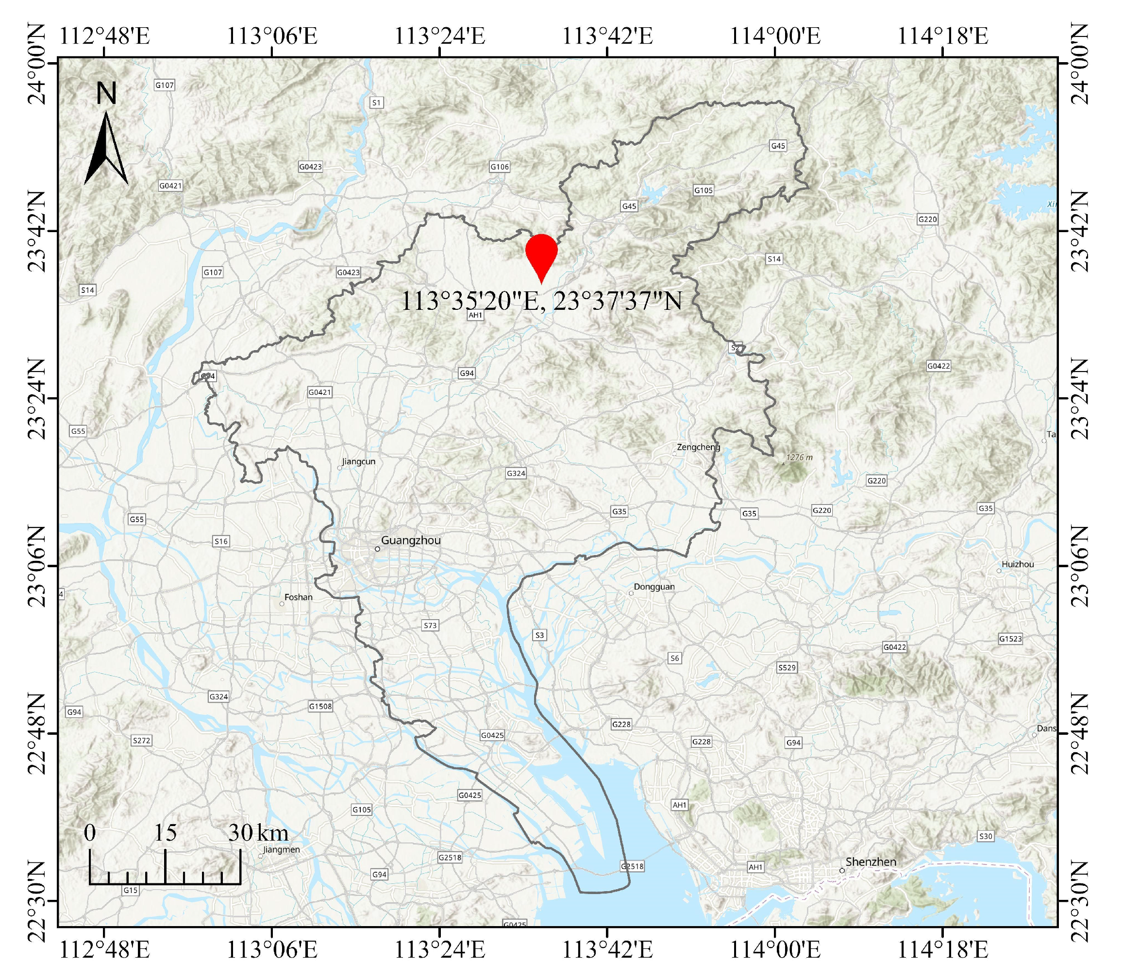
2.1. Collection of Blueberry Samples

In this study, two batches of blueberries from different harvest seasons were collected: 364 samples were collected in April 2024 and 175 samples were collected in March 2025. All blueberry samples selected had a dark appearance and intact surfaces without physical damage. The batch of samples from 2024 were used to establish the model, and the batch of samples from 2025 were used to update the established model and to verify the updated model by calibrated transfer. Both batches were collected from the same blueberry plantation located in Conghua District, Guangzhou, Guangdong Province, China. The geographic location of the experimental site for sampling is marked in Figure 1. All samples were delivered to the same laboratory on the day of harvest for hyperspectral image acquisition and SSC value measurement.

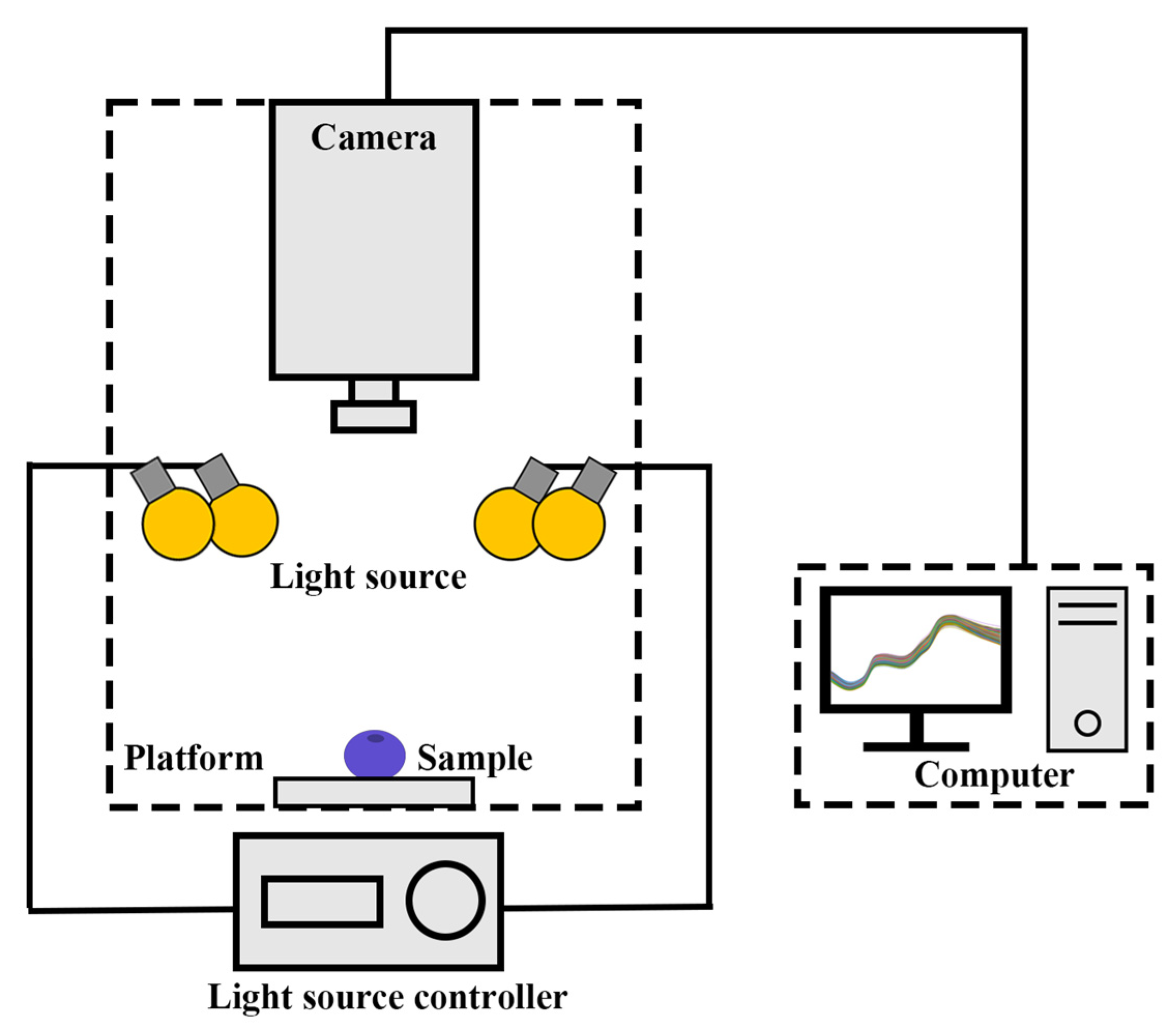
2.2. Hyperspectral Imaging System

The hyperspectral imaging system composed of three major components, these being a hyperspectral camera, light source, and a computer with control software installed. The hyperspectral camera (GaiaField N17E, Dualix Company, Wuxi, China) featured an integrated motor-driven scanning unit that meets the need for scanning hyperspectral cubes. Each hyperspectral cube stacked an image sequence of 512 frames in the range of 900–1700 nm, with a physical spatial resolution of 640 × 666 pixels. The lighting source (HSIA-LST200, Dualix Company, Wuxi, China) had four halogen lamps, covering the spectral range of the hyperspectral camera. The software SpecView 2.9.3.81 was used to control the hyperspectral camera for data collection. The system setup is shown in Figure 2.

To simulate the change in acquisition environmental conditions in practical application scenarios, the light source, exposure time and camera-to-sample distance were changed for collecting two batches of sample data. During the data collection for the 2024 batch, four halogen lamps were all used and the exposure time was set to 1.5 ms, with a camera-to-sample distance of 76.8 cm. For the 2025 batch, only two halogen lamps were turned on, a longer exposure time of 12 ms was adopted, and the camera-to-sample distance was adjusted to 90 cm. As the camera-to-sample distance changed, the focus of the camera was re-adjusted. To improve the stability of the hyperspectral camera and light source, the hyperspectral camera and halogen light source were preheated for 30 min before data acquisition. For each hyperspectral image acquired, a total of 30 blueberry samples were arranged in a 5 × 6 grid configuration (5 columns × 6 rows) on a white Teflon board and imaged simultaneously. The raw hyperspectral images (unprocessed, e.g., no sharpening) were taken from both the stem and calyx sides of each blueberry for subsequent analysis.

2.3. Soluble Solids Content Measurement

After collecting hyperspectral images, the SSC values of the blueberry samples were measured using a digital refractometer (PAL-BX|ACID7; ATAGO Co., Ltd., Tokyo, Japan) with a range of 0–60 °Brix and accuracy of ±0.1 °Brix. The blueberries were juiced and filtered, and the juice was dropped onto the refractometer for measurement. The average of three measurements was taken as the SSC value for each sample for analysis.

2.4. Hyperspectral Image Correction and Spectrums Extraction

The raw hyperspectral images were first corrected to obtain relative reflectance hyperspectral images using Equation (1) [33]:

$$R={\displaystyle \frac{I-D}{W-D}}$$

(1)

where $R$ is the relative reflectance hyperspectral image, $I$ is the hyperspectral image, $D$ is the dark frame obtained by covering the camera lens with an opaque cover, and $W$ is the white frame obtained from a standard whiteboard. The black-frame and white-frame images were captured prior to the collection of sample data. For the relative reflectance hyperspectral images, the region of interests (ROIs) of all blueberry samples were manually segmented and inspected. Then, the mean reflectance spectra of each sample were calculated from two ROIs that were extracted from the stem and calyx images, respectively [20]. As Beer–Lambert’s law demonstrates that there is a linear correlation between absorbance and component concentration, the absorbance spectra were further converted from the relative reflectance spectra for modeling in accordance with Equation (2):

$$Absorbance={\mathit{log}}_{10}\left({\displaystyle \frac{1}{R}}\right)$$

(2)

where $R$ is the relative reflectance spectrum, and $Absorbance$ is the relative absorbance spectrum.

2.5. Principal Component Analysis Algorithm

Principal component analysis (PCA) is widely used as a unsupervised learning method for dimensionality reduction and to obtain a good perspective on data structure [34]. It transforms the original variables into a set of orthogonal principal components through linear transformations, with these components ordered by their variance contribution. The objectivity and visualization advantages of PCA make it an important diagnostic tool for batch consistency evaluation, quality control, and data standardization.

In this study, the PCA method was performed to reveal the variability in spectral data between different batches of blueberry samples. The primary purpose was to assess the spectral differences caused by potential technical factors (e.g., equipment settings and illumination conditions) or biological variations. By projecting the high-dimensional spectral data into a lower-dimensional space defined by the first few principal components, the PCA score plot visually illustrated the distribution and separation patterns between batches. The first principal component (PC1) captures the direction of maximum variance in the dataset, reflecting the most dominant variation among samples. The second principal component (PC2) is orthogonal to PC1 and captures the second-highest variance, representing another independent source of variability. The third principal component (PC3) accounts for additional variation not explained by PC1 and PC2. These components summarize the major sources of spectral variability.

2.6. Data Preprocessing

Due to significant noise interference at both ends of the blueberry spectral data in the 900–1700 nm range, spectral channels at both ends were excluded. The selected spectral data range was from 998 to 1648 nm, covering 395 spectral channels. Statistical analysis was performed on the partitioned dataset to ensure the validity of the sample division. Given the presence of baseline shifts and spectral scattering issues during the original spectral data acquisition, preprocessing was attempted to mitigate the impact of these factors [35,36,37]. In this study, three preprocessing methods were compared: SNV, Savitzky–Golay smoothing (SG), and vector normalization (VN). SNV standardizes the data by subtracting the mean and dividing by the standard deviation for each sample to eliminate scattering effects, and is commonly used in near-infrared spectral data preprocessing. SG is a smoothing and denoising method based on local polynomial fitting that retains higher-order derivative features of the signal and is suitable for noise reduction in spectral or chromatographic data. VN scales the data to a unified range (such as [0, 1] or a vector with a unit length), eliminating dimensional differences and enhancing the reliability of comparative analysis across different samples or features.

The sample partitioning based on the joint X–Y distances (SPXY) method was used to divide the dataset into calibration and prediction sets. SPXY, derived from the Kennard–Stone algorithm, is suitable for dividing a dataset into calibration and prediction sets. Its main goal is to ensure that the distributions of feature space (X) and target variable space (Y) remain consistent during the data splitting process [38]. SPXY ensures representative distributions in both the calibration and prediction sets, thereby enhancing the model’s generalization ability and predictive performance.

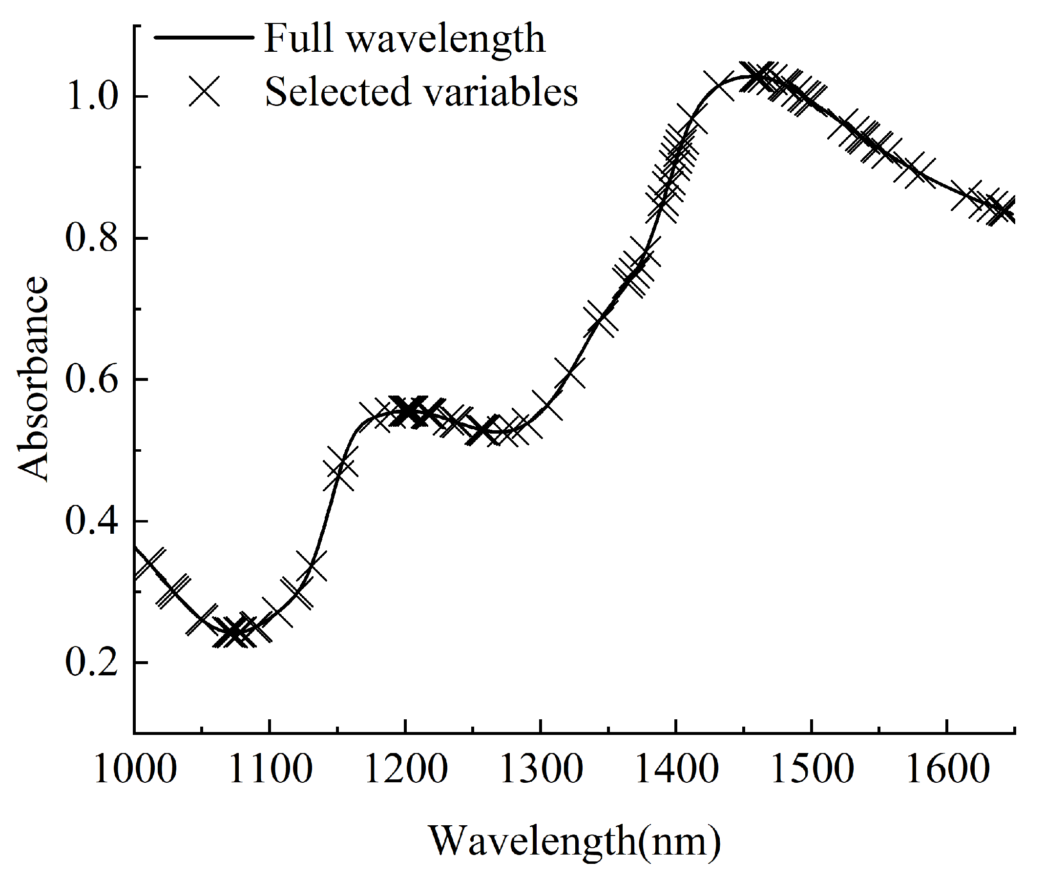
2.7. Feature Wavelength Selection Algorithm

Full-wavelength spectral data contain a large amount of redundant information, including many collinear wavelengths that affect modeling time and accuracy. To improve model accuracy and computational efficiency, it is necessary to select feature wavelengths to reduce dimensionality [39,40]. The spectral data used in this study include 395 spectral channels. The CARS algorithm was used for feature wavelength selection, and the contribution of each wavelength was calculated using 5-fold cross-validation, with the wavelengths contributing the most being selected for the final model construction, thereby improving model accuracy and reducing computational load.

CARS is an effective variable selection method that combines Monte Carlo sampling with PLSR to identify key wavelengths in complex spectral datasets. The algorithm iteratively samples calibration subsets and computes regression coefficients using PLSR. Then, based on an exponential decay function and an adaptive re-weighting mechanism, the importance of variables is determined, and they are ranked and eliminated. CARS improves model performance by retaining informative features while removing noise and irrelevant variables. Its ability to balance predictive accuracy and model robustness makes it particularly suitable for chemometric analysis and high-dimensional regression tasks [41].

2.8. Modeling Algorithms and Evaluation Criteria

PLSR is a data analysis method used for handling highly correlated predictor variables and multiple response variables [42]. PLSR identifies the maximum variance direction between predictor variables and response variables, establishing a predictive model using 5-fold cross-validation. This method is particularly suitable for high-dimensional data analysis and addressing multicollinearity issues. PLSR effectively removes noise from the data while retaining the most informative features for model prediction. PLSR is widely used in chemometrics, biomedical fields, and food science, particularly for spectral analysis [43,44,45].

The evaluation metrics used for the model include the root mean square error of calibration (RMSEC), the coefficient of determination of the calibration set (${\mathrm{R}}_{\mathrm{C}}^2$), RMSEP, ${\mathrm{R}}_{\mathrm{P}}^2$, and the Residual Prediction Deviation (RPD). The optimal model is selected based on the minimum RMSEP and maximum ${\mathrm{R}}_{\mathrm{P}}^2$ principles. RMSE indicates the difference between predicted and actual values, with smaller RMSE values indicating more accurate predictions. $R^2$ represents the goodness-of-fit between the model and the data, ranging from 0 to 1, with values closer to 1 indicating better fit. The formulas for RMSE and $R^2$ are given in Equations (3) and (4), respectively. RPD is defined as the ratio of the standard deviation (SD) of reference values to the RMSEP, as shown in Equation (5). It is widely used in spectral analysis to evaluate the predictive performance of regression models. An RPD value greater than 2.0 indicates acceptable predictive ability, and a value greater than 3.0 indicates good quantitative prediction performance.

$$RMSE=\sqrt{{\displaystyle \frac{1}{n}}{\displaystyle \sum }_{i=1}^n{\left(y_i-{\widehat{y}}_i\right)}^2}$$

(3)

$$R^2=1-{\displaystyle \frac{{{\displaystyle \sum }}_{i=1}^n{\left(y_i-{\widehat{y}}_i\right)}^2}{{{\displaystyle \sum }}_{i=1}^n{\left(y_i-\overline{y}\right)}^2}}$$

(4)

$$RPD={\displaystyle \frac{SD}{RMSEP}}$$

(5)

where $y_i$ represents the true value; ${\widehat{y}}_i$ represents the predicted value; $\overline{y}$ represents the mean value of the sample; $SD$ represents the standard deviation of the reference value; RMSEP represents the root mean square error of prediction.

2.9. Calibration Transfer Strategy

To adapt a model built using samples from an old batch for predictions in a new batch, the SS-PFCE algorithm was applied for calibration transfer. The SS-PFCE algorithm is suitable for scenarios where an established model needs to be adapted to a new dataset, using only a small portion of the samples from the new dataset for model transfer [30]. This method alleviates the impact of spectral differences caused by factors such as different batches, geographic conditions, and aging of hyperspectral instruments on prediction performance. It allows for improved generalizability of the old model and maintains sufficient model performance without the need to reacquire a large amount of new batch sample data for re-modeling. The principle of the SS-PFCE algorithm is described in Equation (6), where a correlation constraint is introduced to prevent overfitting.

$$\underset{b_{0,s},b_s}{\min }\left(\Vert y-\left[1X_s\right]\left[\begin{array}{c}{b}_{0,s}\\ b_s\end{array}\right]{\Vert }^2\right)$$

(6)

$$s.t.corr\left(b_s,b_m\right)>r_{th}$$

where $X_s$ represents the spectra of new samples, $y$ denotes the reference values of new samples, $b_m$ is the regression coefficient vector of the old model, $b_s$ is the coefficient vector of the new model, $b_{0,s}$ is the intercept of the new model, $corr$ is the function for computing the correlation coefficient, and $r_{th}$ is the predefined threshold for correlation.

In this study, all data analysis steps were implemented using Python 3.11.7.

3. Results

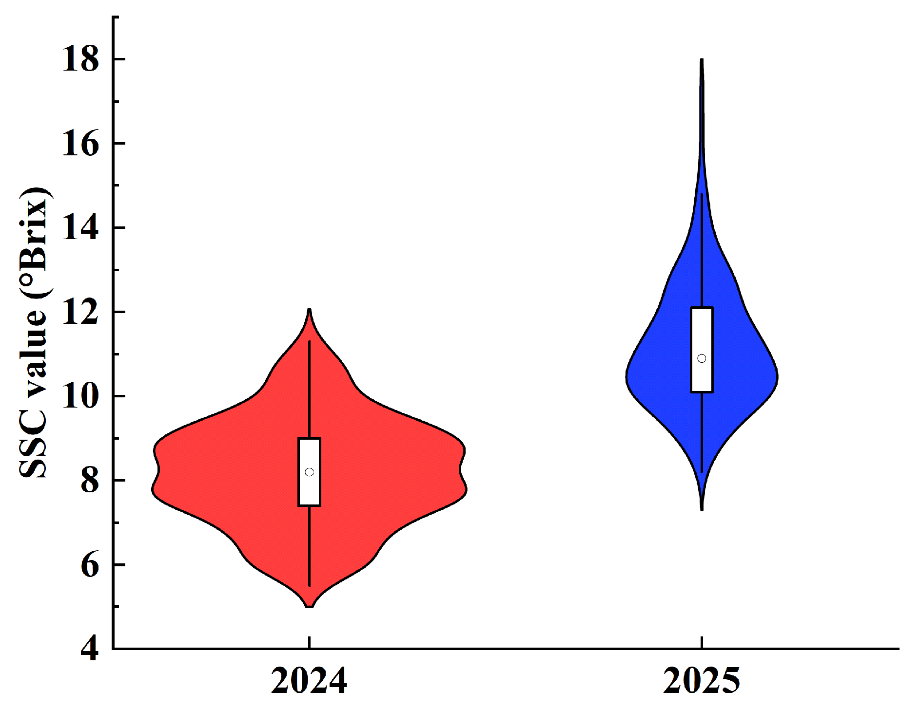
3.1. Sample Sets Division

Before modeling, the SPXY method was used to partition the blueberry samples from two different years into training and prediction datasets. A total of 364 samples from the 2024 batch were used for model construction, with a calibration-to-prediction ratio of 3:1. For the 2025 batch, 175 samples were divided in a 1:3 ratio between the calibration and prediction sets, with 44 samples used for calibration transfer and 131 samples used for validating the model’s performance after calibration transfer. The minimum, maximum, mean, and standard deviation values for the calibration and prediction sets are shown in

Table 1. SPXY sample set division results.

Year of Sample	Sample Set	Number of Samples	Minimum	Maximum	Average Value	Standard Deviation
2024	Calibration Set	273	5.5	11.5	8.23	1.31
	Prediction Set	91	5.7	11.2	8.16	1.15
	Total Samples	364	5.5	11.5	8.21	1.27
2025	Calibration Set	44	8.2	17.4	11.78	2.08
	Prediction Set	131	8.7	14.7	10.96	1.21
	Total Samples	175	8.2	17.4	11.17	1.52

. The average SSC of the 2025 batch samples was 2.96 °Brix higher than that of the 2024 batch samples, but the standard deviation was also greater. In the 2024 batch, the SSC range for the calibration set was 5.5–11.5 °Brix. In the 2025 batch, the calibration set had an SSC range of 8.2–17.4 °Brix. Figure 3 shows the violin plots of the SSC distribution for the 2024 (red) and 2025 (blue) batches. As can be seen, there was a significant difference in SSC between the two batches, with the 2025 batch samples being noticeably sweeter than the 2024 batch.

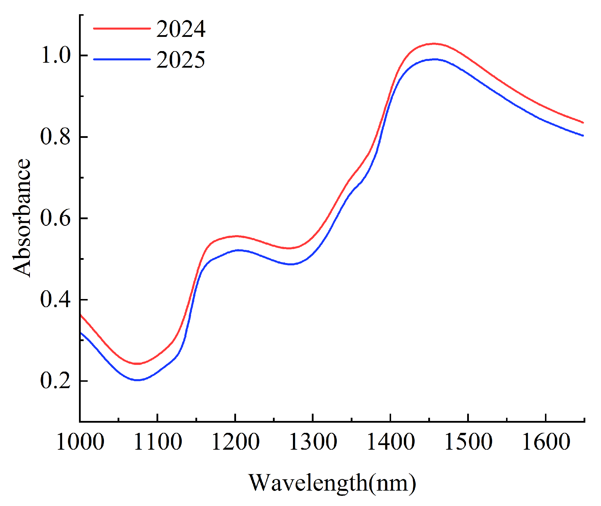
3.2. Spectral Analysis

The absorbance spectra for the 2024 and 2025 batches are shown in Figure 4, with a wavelength range of 998–1648 nm. Two distinct absorption peaks can be observed, located near 1190 nm and 1450 nm. For instance, fructose in blueberries exhibits stretching vibrations of C-H chemical bonds. The absorption peak near 1190 nm is related to the second overtone of the C-H bond, while the dip near 1450 nm corresponds to the first overtone of the O-H bond [46,47]. It is also noticeable that the absorbance values for the two batches differ, with the 2024 batch having higher absorbance values than the 2025 batch.

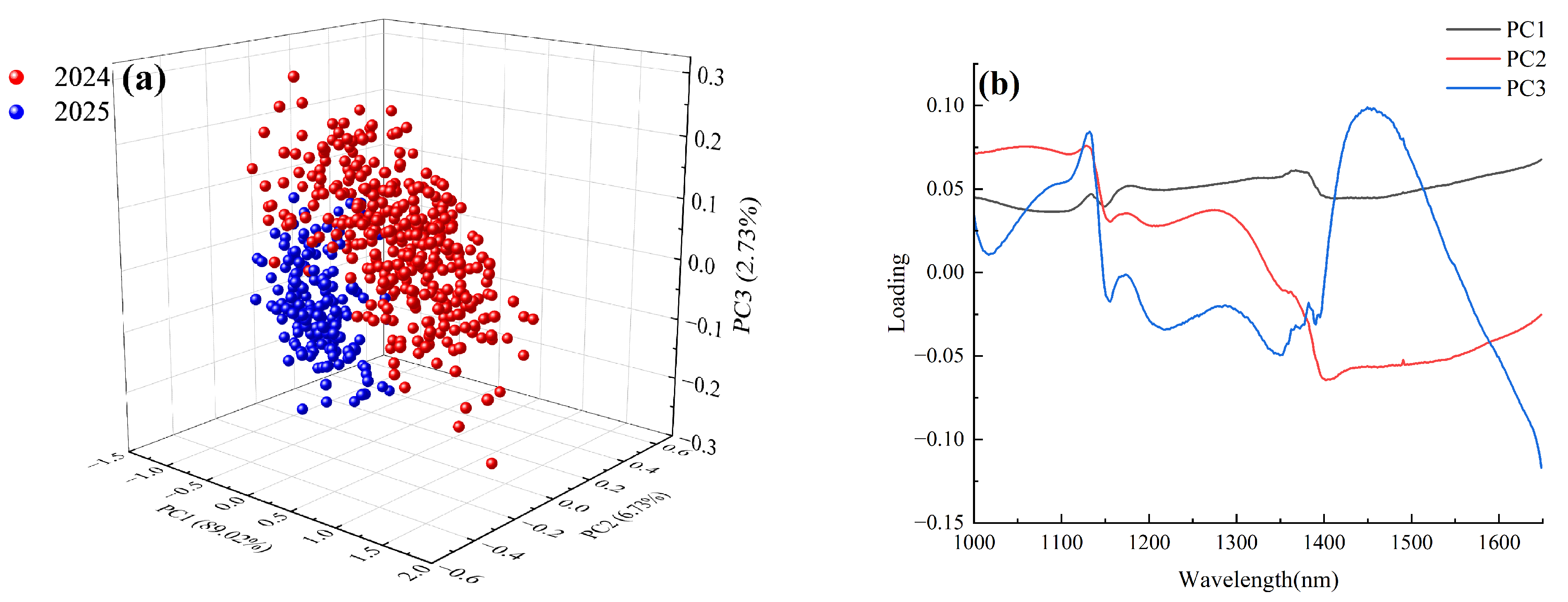
3.3. Principal Component Analysis

To evaluate the spectral differences between the two batches of blueberry samples, the raw spectra from the 2024 and 2025 batches were merged. Then, the combined spectral matrix was operated using PCA for inspecting the main variance trends across samples.

Figure 5a shows the distribution of the first three principal components of the spectral matrix. The three principal components plotted accounted for a cumulative variance contribution of 98.48%, where PC1 explained 89.02%, PC2 explained 6.73%, and PC3 explained 2.73%. Obviously, the samples from the 2024 and 2025 batches formed two large intervals of clusters, indicating batch-specific spectral differences. This separation reflected differences in sample properties and acquisition conditions, such as lighting setup and hyperspectral camera adjustments. By viewing the corresponding loading plots of first three principal components in Figure 5b, the loading values could be used to further identify the spectral regions that resulted in the variability. The loadings of PC1 were all greater than zero, which more often represented baseline shifts in the spectra, corresponding to shift phenomena of the average spectra in Figure 4. The loadings curve of PC3 formed peaks near 1125 nm and 1450 nm, representing the second overtone vibration absorption and first overtone combination vibration absorption of the functional groups -CH3 and CH, respectively. This likely reflects the differential characteristics of the sample components. Overall, the large intervals of clusters highlighted the potential challenge in directly transferring models between batches.

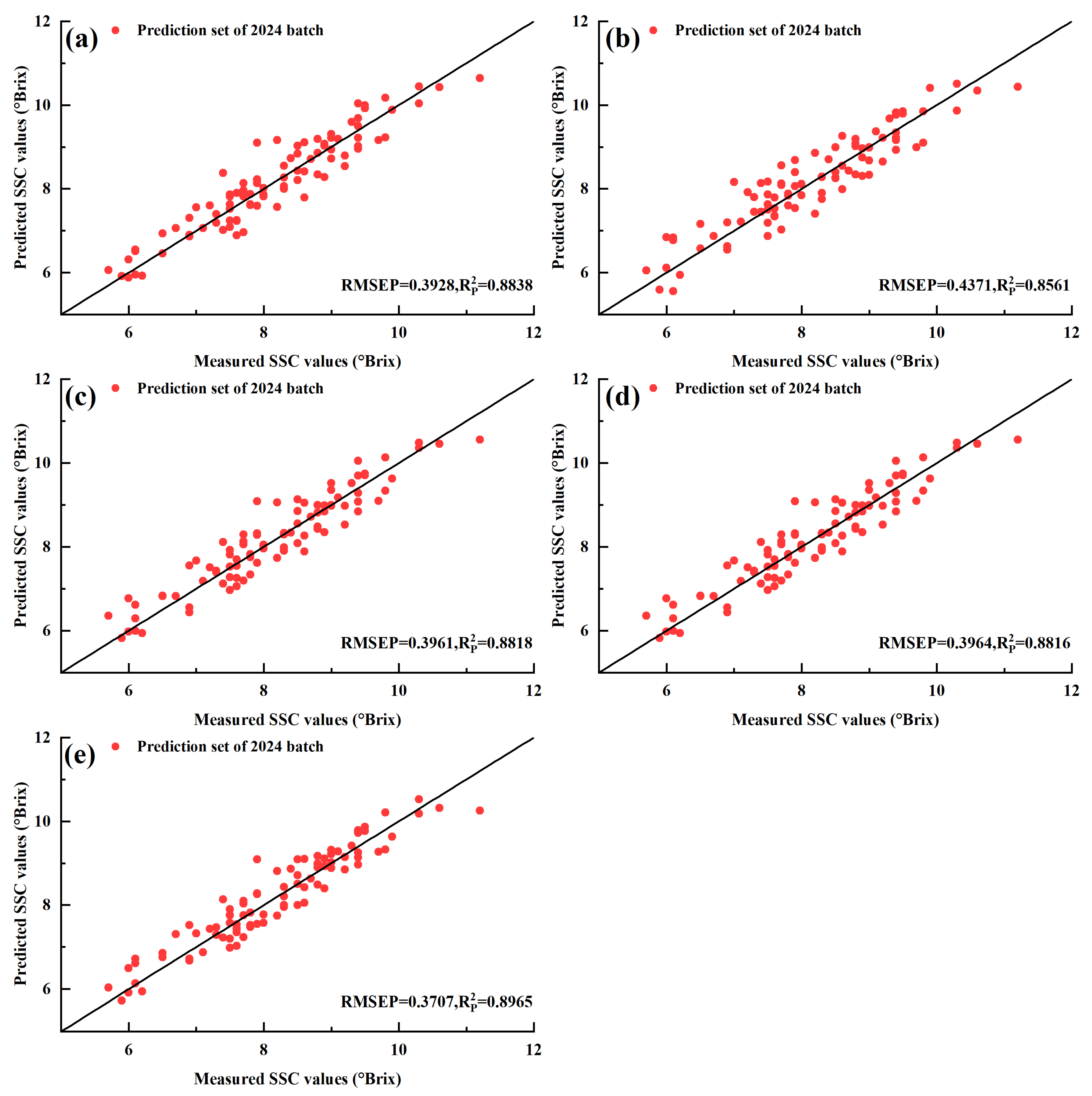
3.4. Spectral Data Preprocessing and PLSR Model Construction

To minimize the influence of irrelevant information and noise on the spectral data, preprocessing and CARS feature wavelength selection were employed to reduce computational load and enhance model performance [48]. A PLSR model with five-fold cross-validation was applied to the 2024 batch dataset, and the best preprocessing method was selected by comparing ${\mathrm{R}}_{\mathrm{P}}^2$ and RMSEP values. The raw spectral data (RAW) and three different preprocessing methods (SNV, SG, and VN) were used as input variables for the PLSR model, and corresponding SSC prediction models were built. The maximum number of latent variables (LVs) for the PLSR models was set to 40, and grid search was used to find the best LVs. The results of the PLSR modeling are shown in

Table 2. PLSR modeling results after preprocessing with different methods.

Preprocessing Methods	Number of Features	LVs	RMSEC	${\mathbf{R}}_{\mathbf{C}}^2$	RMSEP	${\mathbf{R}}_{\mathbf{P}}^2$	RPD
RAW	395	31	0.3192	0.9405	0.3928	0.8838	2.95
SNV	395	27	0.3726	0.9189	0.4371	0.8561	2.65
SG	395	31	0.3295	0.9366	0.3961	0.8818	2.93
VN	395	25	0.3509	0.9281	0.3964	0.8816	2.93
RAW-CARS	88	30	0.3191	0.9405	0.3707	0.8965	3.13

.

As shown in Table 2, the model built using raw spectral data achieved the best performance, with an RMSEP of 0.3928, an ${\mathrm{R}}_{\mathrm{P}}^2$ of 0.8838, and an RPD of 2.95. The other three models exhibited varying degrees of performance degradation, particularly the SNV-preprocessed model. The superior performance of the raw spectral data model compared to that of preprocessed spectral data models may be attributed to the combined spectral data from both the calyx and stem sides of blueberries, which enhanced the stability of the raw data. Consequently, preprocessing the raw spectral data using these three methods might have removed some useful information, leading to reduced PLSR modeling performance. CARS was used to select feature wavelengths from the raw spectral data. The original number of wavelengths was 395, while the selected number after CARS was 88, accounting for 22.2% of the full wavelengths. Table 2 demonstrates that the PLSR model based on CARS-selected feature wavelengths showed improved performance in both RMSEP and ${\mathrm{R}}_{\mathrm{P}}^2$. Specifically, the RMSEP decreased to 0.3707, the ${\mathrm{R}}_{\mathrm{P}}^2$ increased to 0.8965, and the RPD exceeded 3, indicating highly reliable predictive performance. Figure 6 presents the prediction scatter plots of the PLSR models using different preprocessing methods. Figure 7 shows the distribution of feature wavelengths selected by CARS.

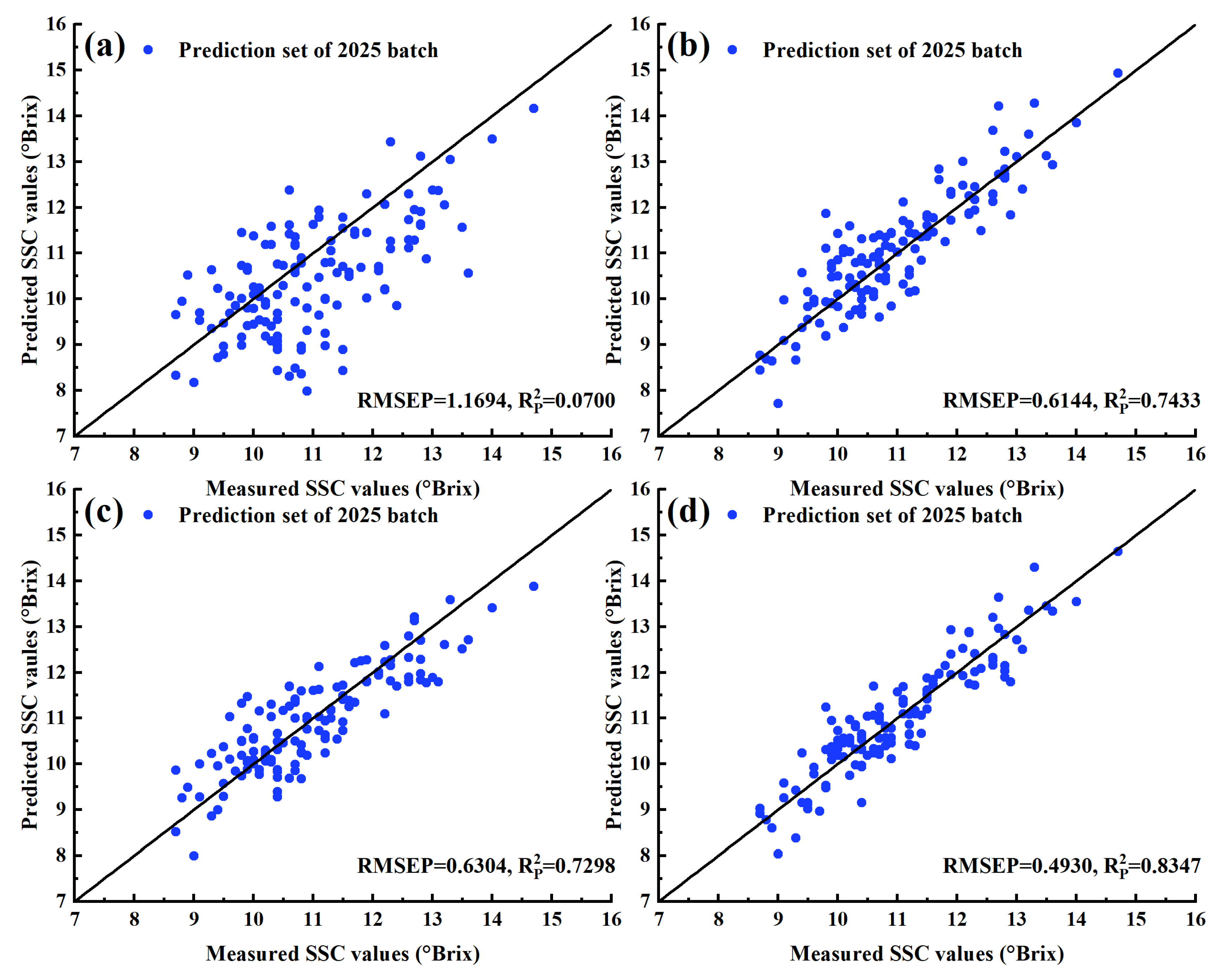
3.5. Models Updated with Calibration Transfer Strategy Using SS-PFCE

Due to the poor prediction performance of the established PLSR model with regard to the SSC of the new batch of blueberry samples, calibration transfer was performed using the 2025 batch calibration set (44 blueberry samples, accounting for 25% of the 2025 batch) through the SS-PFCE algorithm, resulting in the SS-PFCE model. To compare the difference between calibration transfer and re-modeling, a new PLSR model was reconstructed using only the 2025 batch calibration set. Additionally, the calibration sets of the 2024 and 2025 batches were combined (with 2025 batch samples accounting for 13.9% of the combined set) to build a generalized PLSR model. The prediction set from the 2025 batch (131 blueberry samples, accounting for 75% of the batch) was used to evaluate the model performance. The modeling results are shown in

Table 3. Modeling results of the SS-PFCE model and the two newly constructed PLSR models.

Model	Calibration Year	Calibration Set Size	RMSEC	${\mathbf{R}}_{\mathbf{C}}^2$	RMSEP	${\mathbf{R}}_{\mathbf{P}}^2$	RPD
PLSR	2024	273	1.3260	0.5919	1.1694	0.0700	1.04
PLSR	2025	44	0.1598	0.9941	0.6144	0.7433	1.98
PLSR	2024 + 2025	317	0.5427	0.9176	0.6304	0.7298	1.93
SS-PFCE	2025	44	0.3886	0.9650	0.4930	0.8347	2.47

.

As presented in Table 3, the PLSR model developed using the 2024 batch calibration set exhibited poor predictive performance when directly applied to the 2025 batch prediction set, with RMSEP and R2 values of 1.1694 and 0.0700, respectively. The newly constructed PLSR model using only the 2025 calibration set yielded an RMSEC of 0.1598 and an ${\mathrm{R}}_{\mathrm{C}}^2$ of 0.9941, but its RMSEP and ${\mathrm{R}}_{\mathrm{P}}^2$ were 0.6144 and 0.7433, respectively, indicating a certain degree of overfitting. This may be attributed to the limited number of samples (44) used in the calibration set, which was insufficient to provide adequate reference information. When combining the 2024 and 2025 calibration sets, the generalized PLSR model showed an RMSEP of 0.6304, an ${\mathrm{R}}_{\mathrm{P}}^2$ of 0.7298, and an RPD of 1.93. Although the generalized PLSR model reduced overfitting to some extent, its prediction performance remained inferior to the SS-PFCE model. The RPD values of both reconstructed models were below 2, indicating poor usability. The SS-PFCE model, which was obtained via calibration transfer from the PLSR model, still achieved satisfactory prediction performance. The SS-PFCE model yielded an RMSEP of 0.4930 and an ${\mathrm{R}}_{\mathrm{P}}^2$ of 0.8347, with an RPD of 2.47. Figure 8 illustrates the differences in prediction results before and after calibration transfer. It is evident from the plots that the prediction points of the SS-PFCE model are more concentrated than those of the other models. Figure 9 presents the regression coefficients before and after calibration transfer. As can be observed from the figure, the PLSR model and SS-PFCE model exhibit generally consistent trends in their regression coefficients. This consistency indicates that the spectral characteristics of functional groups directly associated with the SSC remain similar across different sample batches. The larger absolute values of regression coefficients in the SS-PFCE model after calibration transfer may be attributed to adjustments in experimental instrumentation. Additionally, the 2025 batch samples showed significant distributional differences in SSC compared to the 2024 batch samples, necessitating model recalibration of regression coefficients to adapt to the new data distribution. Overall, the SS-PFCE model outperformed the other models, indicating that an established blueberry SSC prediction model can be effectively adapted to a new batch using a small number of new samples through calibration transfer, achieving desirable performance.

4. Discussion

Hyperspectral imaging plays an essential role in non-destructive testing of agricultural products. Selecting an appropriate wavelength range enables accurate detection of internal quality attributes such as SSC, moisture content, and anthocyanin levels. However, differences in hyperspectral instruments, environmental conditions, and cultivation practices often compromise model transferability.

In this study, statistical analysis of SSC values revealed significant differences between the two batches. Despite the identical variety, picking location, and maturity season of the blueberries, the SSC still showed a notable batch effect, likely due to variations in light exposure and irrigation during ripening. This study simulated environmental variations in practical scenarios by adjusting the number of light sources and modifying the camera-to-sample distance and exposure time. Regarding spectral variability, Meng et al. [21] conducted PCA on three blueberry cultivars and found shared spectral characteristics. Similarly, PCA in this study revealed pronounced spectral differences between the two batches. The observed differences in SSC values and spectral data between batches still present challenges for model transferability.

After black-and-white correction of the hyperspectral image data, spectral information from both the stem and calyx sides of each fruit was extracted. The average spectral data of all pixels within each region were calculated and then combined, effectively minimizing noise. Further averaging across both sides reduced interference even more, which may explain why the raw spectra outperformed preprocessed data in model building. In SSC prediction, appropriate spectral dimensionality reduction methods and modeling approaches are crucial for enhancing prediction efficiency and performance [20,49]. In this study, the CARS algorithm reduced the original 395 wavelengths to 88, eliminating redundancy and improving the PLSR model (RMSEP and ${\mathrm{R}}_{\mathrm{P}}^2$ improved from 0.3928 and 0.8838 to 0.3707 and 0.8965, respectively; RPD increased from 2.95 to 3.13). This robust baseline facilitated the development of high-performance calibration transfer models.

As shown in Table 3 and Figure 8, the PLSR model built with the 2024 batch performed poorly on the 2025 batch, indicating a need for model updating. Prior studies have shown that the SS-PFCE algorithm outperforms methods like PDS and SST [30]. Therefore, SS-PFCE was applied using a small subset of 2025 samples to transfer the existing PLSR model. For comparison, two new PLSR models were constructed. It can be observed from Table 3 and Figure 8 that the SS-PFCE model demonstrated a significant advantage, achieving RMSEP and ${\mathrm{R}}_{\mathrm{P}}^2$ values of 0.4930 and 0.8347, respectively, with an RPD of 2.47 using only 44 new samples. While building a new model with sufficient samples can yield higher accuracy, it is time- and labor-intensive. SS-PFCE offers a practical solution for adapting existing models with minimal new data. Similar success was reported by Mishra et al. [31] for pear and kiwifruit SSC prediction across batches using SS-PFCE and small calibration sets. Geng et al. [50] found in their experiment that the spectral data of tobacco powder and tobacco filament exhibited significant differences. Although the spectral trends of the two forms of tobacco samples were similar, their amplitudes differed. Calibration transfer was subsequently performed using the NS-PFCE algorithm, which ultimately enabled the SSC prediction model developed based on tobacco powder samples to be successfully applied to tobacco filament. Similarly, in the present study, the spectral data of the two batches of blueberries also showed similar trends but different amplitudes. This discrepancy was effectively eliminated through calibration transfer using the SS-PFCE algorithm, thereby reducing the prediction error caused by spectral differences. Regarding the cross-cultivar prediction of blueberry SSC, Meng et al. [21] developed a universal model by incorporating spectral data from three blueberry cultivars. However, universal models may still exhibit varying degrees of predictive performance deterioration when applied to new sample batches due to instrumental aging and environmental variations. In comparison, the calibration transfer strategy employed in this study effectively eliminated batch effects and significantly improved the prediction performance of the established blueberry SSC model on new batches, thereby demonstrating enhanced feasibility and practical application value.

Although the SS-PFCE algorithm demonstrated effectiveness in improving the predictive performance of our model across different batches, its practical application may be constrained by the exclusive use of samples from a single blueberry cultivar cultivated at one plantation site. This sampling limitation raises concerns about the model’s generalizability to other cultivars. Furthermore, the current research did not examine the model’s performance in cross-cultivar calibration transfer scenarios, which represents a critical area for future investigation to enhance the broader applicability of this approach.

5. Conclusions

This study investigated the transferability of an established blueberry SSC non-destructive detection model across different sample batches. The model built using 2024 batch samples performed well on the same batch but poorly on the 2025 batch. By applying SS-PFCE with a small number of 2025 samples, the original model was effectively adapted for SSC prediction in the new batch, significantly reducing the time and labor costs of re-modeling. Compared to rebuilding models, calibration transfer via SS-PFCE demonstrated clear advantages, yielding strong predictive performance.

The combination of hyperspectral imaging and machine learning provides a powerful approach for internal quality evaluation in fruits. However, achieving high predictive accuracy typically requires extensive data collection. This study offers valuable insights into the cross-batch transferability of blueberry SSC models. Rather than building separate models for each cultivar and batch, calibration transfer based on existing models is more practical for real-world applications. While this study focused on a single cultivar, it lays the foundation for future research into more generalizable models for SSC detection across various varieties and batches.

References

1. Wang, Y.; Zhang, Q.; Cui, M.-Y.; Fu, Y.; Wang, X.-H.; Yang, Q.; Zhu, Y.; Yang, X.-H.; Bi, H.-J.; Gao, X.-L. Aroma enhancement of blueberry wine by postharvest partial dehydration of blueberries. Food Chem. 2023, 426, 136593. [Google Scholar] [CrossRef] [PubMed]
2. Stull, A.J.; Cassidy, A.; Djousse, L.; Johnson, S.A.; Krikorian, R.; Lampe, J.W.; Mukamal, K.J.; Nieman, D.C.; Porter Starr, K.N.; Rasmussen, H.; et al. The state of the science on the health benefits of blueberries: A perspective. Front. Nutr. 2024, 11, 1415737. [Google Scholar] [CrossRef] [PubMed]
3. Sivapragasam, N.; Neelakandan, N.; Rupasinghe, H.P.V. Potential health benefits of fermented blueberry: A review of current scientific evidence. Trends Food Sci. Technol. 2023, 132, 103–120. [Google Scholar] [CrossRef]
4. Rashwan, A.K.; Osman, A.I.; Karim, N.; Mo, J.; Chen, W. Unveiling the Mechanisms of the Development of Blueberries-Based Functional Foods: An Updated and Comprehensive Review. Food Rev. Int. 2023, 40, 1913–1940. [Google Scholar] [CrossRef]
5. Liu, J.; Wang, Q.; Weng, L.; Zou, L.; Jiang, H.; Qiu, J.; Fu, J. Analysis of sucrose addition on the physicochemical properties of blueberry wine in the main fermentation. Front. Nutr. 2023, 9, 1092696. [Google Scholar] [CrossRef]
6. Wang, X.; Cheng, J.; Zhu, Y.; Li, T.; Wang, Y.; Gao, X. Intermolecular copigmentation of anthocyanins with phenolic compounds improves color stability in the model and real blueberry fermented beverage. Food Res. Int. 2024, 190, 114632. [Google Scholar] [CrossRef]
7. Mishra, G.; Sahni, P.; Pandiselvam, R.; Panda, B.K.; Bhati, D.; Mahanti, N.K.; Kothakota, A.; Kumar, M.; Cozzolino, D. Emerging nondestructive techniques to quantify the textural properties of food: A state-of-art review. J. Texture Stud. 2023, 54, 173–205. [Google Scholar] [CrossRef]
8. He, Y.; Xiao, Q.; Bai, X.; Zhou, L.; Liu, F.; Zhang, C. Recent progress of nondestructive techniques for fruits damage inspection: A review. Crit. Rev. Food Sci. Nutr. 2021, 62, 5476–5494. [Google Scholar] [CrossRef]
9. Chen, Z.; Wang, J.; Liu, X.; Gu, Y.; Ren, Z. The Application of Optical Nondestructive Testing for Fresh Berry Fruits. Food Eng. Rev. 2023, 16, 85–115. [Google Scholar] [CrossRef]
10. Li, L.; Hu, D.-Y.; Tang, T.-Y.; Tang, Y.-L. Non-destructive detection of the quality attributes of fruits by visible-near infrared spectroscopy. J. Food Meas. Charact. 2022, 17, 1526–1534. [Google Scholar] [CrossRef]
11. Cevoli, C.; Iaccheri, E.; Fabbri, A.; Ragni, L. Data fusion of FT-NIR spectroscopy and Vis/NIR hyperspectral imaging to predict quality parameters of yellow flesh “Jintao” kiwifruit. Biosyst. Eng. 2024, 237, 157–169. [Google Scholar] [CrossRef]
12. Zhao, Y.; Zhou, L.; Wang, W.; Zhang, X.; Gu, Q.; Zhu, Y.; Chen, R.; Zhang, C. Visible/near-infrared Spectroscopy and Hyperspectral Imaging Facilitate the Rapid Determination of Soluble Solids Content in Fruits. Food Eng. Rev. 2024, 16, 470–496. [Google Scholar] [CrossRef]
13. Rodríguez-Ortega, A.; Aleixos, N.; Blasco, J.; Albert, F.; Munera, S. Study of light penetration depth of a Vis-NIR hyperspectral imaging system for the assessment of fruit quality. A case study in persimmon fruit. J. Food Eng. 2023, 358, 111673. [Google Scholar] [CrossRef]
14. Hasanzadeh, B.; Abbaspour-Gilandeh, Y.; Soltani-Nazarloo, A.; Hernández-Hernández, M.; Gallardo-Bernal, I.; Hernández-Hernández, J.L. Non-Destructive Detection of Fruit Quality Parameters Using Hyperspectral Imaging, Multiple Regression Analysis and Artificial Intelligence. Horticulturae 2022, 8, 598. [Google Scholar] [CrossRef]
15. Benelli, A.; Cevoli, C.; Ragni, L.; Fabbri, A. In-field and non-destructive monitoring of grapes maturity by hyperspectral imaging. Biosyst. Eng. 2021, 207, 59–67. [Google Scholar] [CrossRef]
16. Li, X.; Wei, Z.; Peng, F.; Liu, J.; Han, G. Non-destructive prediction and visualization of anthocyanin content in mulberry fruits using hyperspectral imaging. Front. Plant Sci. 2023, 14, 1137198. [Google Scholar] [CrossRef]
17. Wang, B.; Yang, H.; Li, L.; Zhang, S. Non-Destructive Detection of Cerasus Humilis Fruit Quality by Hyperspectral Imaging Combined with Chemometric Method. Horticulturae 2024, 10, 519. [Google Scholar] [CrossRef]
18. Chen, G.; Yang, M.; Wang, G.; Dai, J.; Yu, S.; Chen, B.; Liu, D. Exploring a universal model for predicting blueberry soluble solids content based on hyperspectral imaging and transfer learning to address spatial heterogeneity challenge. Spectrochim. Acta Part A Mol. Biomol. Spectrosc. 2025, 334, 125921. [Google Scholar] [CrossRef]
19. K.S., S.; George, S.N.; O.V., A.C.; K.M., J.; P., K.; Francis, J.; George, S. NorBlueNet: Hyperspectral imaging-based hybrid CNN-transformer model for non-destructive SSC analysis in Norwegian wild blueberries. Comput. Electron. Agric. 2025, 235, 110340. [Google Scholar] [CrossRef]
20. Qiu, G.; Chen, B.; Lu, H.; Yue, X.; Deng, X.; Ouyang, H.; Li, B.; Wei, X. Nondestructively Determining Soluble Solids Content of Blueberries Using Reflection Hyperspectral Imaging Technique. Agronomy 2024, 14, 2296. [Google Scholar] [CrossRef]
21. Meng, L.; Chen, G.; Liu, D.; Tian, N. Universal Modeling for Non-Destructive Testing of Soluble Solids Content in Multi-Variety Blueberries Based on Hyperspectral Imaging Technology. Appl. Sci. 2025, 15, 3888. [Google Scholar] [CrossRef]
22. Çetin, N.; Karaman, K.; Kavuncuoğlu, E.; Yıldırım, B.; Jahanbakhshi, A. Using hyperspectral imaging technology and machine learning algorithms for assessing internal quality parameters of apple fruits. Chemom. Intell. Lab. Syst. 2022, 230, 104650. [Google Scholar] [CrossRef]
23. Ebrahimi, S.; Pourdarbani, R.; Sabzi, S.; Rohban, M.H.; Arribas, J.I. From Harvest to Market: Non-Destructive Bruise Detection in Kiwifruit Using Convolutional Neural Networks and Hyperspectral Imaging. Horticulturae 2023, 9, 936. [Google Scholar] [CrossRef]
24. Cho, B.-H.; Lee, K.-B.; Hong, Y.; Kim, K.-C. Determination of Internal Quality Indices in Oriental Melon Using Snapshot-Type Hyperspectral Image and Machine Learning Model. Agronomy 2022, 12, 2236. [Google Scholar] [CrossRef]
25. Kim, M.-J.; Yu, W.-H.; Song, D.-J.; Chun, S.-W.; Kim, M.S.; Lee, A.; Kim, G.; Shin, B.-S.; Mo, C. Prediction of Soluble-Solid Content in Citrus Fruit Using Visible–Near-Infrared Hyperspectral Imaging Based on Effective-Wavelength Selection Algorithm. Sensors 2024, 24, 1512. [Google Scholar] [CrossRef] [PubMed]
26. Qiu, G.; Lu, H.; Wang, X.; Wang, C.; Xu, S.; Liang, X.; Fan, C. Nondestructive Detecting Maturity of Pineapples Based on Visible and Near-Infrared Transmittance Spectroscopy Coupled with Machine Learning Methodologies. Horticulturae 2023, 9, 889. [Google Scholar] [CrossRef]
27. Wang, Y.; Lysaght, M.J.; Kowalski, B.R. Improvement of multivariate calibration through instrument standardization. Anal. Chem. 1992, 64, 562–564. [Google Scholar] [CrossRef]
28. Du, W.; Chen, Z.-P.; Zhong, L.-J.; Wang, S.-X.; Yu, R.-Q.; Nordon, A.; Littlejohn, D.; Holden, M. Maintaining the predictive abilities of multivariate calibration models by spectral space transformation. Anal. Chim. Acta 2011, 690, 64–70. [Google Scholar] [CrossRef]
29. Liu, Y.; Cai, W.; Shao, X. Linear model correction: A method for transferring a near-infrared multivariate calibration model without standard samples. Spectrochim. Acta Part A Mol. Biomol. Spectrosc. 2016, 169, 197–201. [Google Scholar] [CrossRef]
30. Zhang, J.; Li, B.; Hu, Y.; Zhou, L.; Wang, G.; Guo, G.; Zhang, Q.; Lei, S.; Zhang, A. A parameter-free framework for calibration enhancement of near-infrared spectroscopy based on correlation constraint. Anal. Chim. Acta 2021, 1142, 169–178. [Google Scholar] [CrossRef]
31. Mishra, P.; Woltering, E. Handling batch-to-batch variability in portable spectroscopy of fresh fruit with minimal parameter adjustment. Anal. Chim. Acta 2021, 1177, 338771. [Google Scholar] [CrossRef] [PubMed]
32. Guo, C.; Zhang, J.; Cai, W.; Shao, X. Enhancing Transferability of Near-Infrared Spectral Models for Soluble Solids Content Prediction across Different Fruits. Appl. Sci. 2023, 13, 5417. [Google Scholar] [CrossRef]
33. Benelli, A.; Cevoli, C.; Fabbri, A.; Ragni, L. Ripeness evaluation of kiwifruit by hyperspectral imaging. Biosyst. Eng. 2022, 223, 42–52. [Google Scholar] [CrossRef]
34. Uddin, M.P.; Mamun, M.A.; Hossain, M.A. Effective feature extraction through segmentation-based folded-PCA for hyperspectral image classification. Int. J. Remote Sens. 2019, 40, 7190–7220. [Google Scholar] [CrossRef]
35. Nirere, A.; Sun, J.; Kama, R.; Atindana, V.A.; Nikubwimana, F.D.; Dusabe, K.D.; Zhong, Y. Nondestructive detection of adulterated wolfberry (Lycium Chinense) fruits based on hyperspectral imaging technology. J. Food Process Eng. 2023, 46, 14293. [Google Scholar] [CrossRef]
36. Abenina, M.I.A.; Maja, J.M.; Cutulle, M.; Melgar, J.C.; Liu, H. Prediction of Potassium in Peach Leaves Using Hyperspectral Imaging and Multivariate Analysis. AgriEngineering 2022, 4, 400–413. [Google Scholar] [CrossRef]
37. Haghbin, N.; Bakhshipour, A.; Zareiforoush, H.; Mousanejad, S. Non-destructive pre-symptomatic detection of gray mold infection in kiwifruit using hyperspectral data and chemometrics. Plant Methods 2023, 19, 53. [Google Scholar] [CrossRef]
38. Galvao, R.; Araujo, M.; Jose, G.; Pontes, M.; Silva, E.; Saldanha, T. A method for calibration and validation subset partitioning. Talanta 2005, 67, 736–740. [Google Scholar] [CrossRef]
39. Faqeerzada, M.A.; Kim, Y.-N.; Kim, H.; Akter, T.; Kim, H.; Park, M.-S.; Kim, M.S.; Baek, I.; Cho, B.-K. Hyperspectral imaging system for pre- and post-harvest defect detection in paprika fruit. Postharvest Biol. Technol. 2024, 218, 113151. [Google Scholar] [CrossRef]
40. Khaled, A.Y.; Ekramirad, N.; Donohue, K.D.; Villanueva, R.T.; Adedeji, A.A. Non-Destructive Hyperspectral Imaging and Machine Learning-Based Predictive Models for Physicochemical Quality Attributes of Apples during Storage as Affected by Codling Moth Infestation. Agriculture 2023, 13, 1086. [Google Scholar] [CrossRef]
41. Adesokan, M.; Otegbayo, B.; Alamu, E.O.; Olutoyin, M.A.; Maziya-Dixon, B. Evaluating the dry matter content of raw yams using hyperspectral imaging spectroscopy and machine learning. J. Food Compos. Anal. 2024, 135, 106692. [Google Scholar] [CrossRef]
42. Jahani, T.; Kashaninejad, M.; Ziaiifar, A.M.; Golzarian, M.; Akbari, N.; Soleimanipour, A. Effect of selected pre-processing methods by PLSR to predict low-fat mozzarella texture measured by hyperspectral imaging. J. Food Meas. Charact. 2024, 18, 5060–5072. [Google Scholar] [CrossRef]
43. Ahmed, M.T.; Monjur, O.; Kamruzzaman, M. Deep learning-based hyperspectral image reconstruction for quality assessment of agro-product. J. Food Eng. 2024, 382, 112223. [Google Scholar] [CrossRef]
44. Hitchman, S.; Loeffen, M.P.F.; Reis, M.M.; Craigie, C.R. Robustness of hyperspectral imaging and PLSR model predictions of intramuscular fat in lamb M. longissimus lumborum across several flocks and years. Meat Sci. 2021, 179, 108492. [Google Scholar] [CrossRef] [PubMed]
45. Bai, S.H.; Tootoonchy, M.; Kämper, W.; Tahmasbian, I.; Farrar, M.B.; Boldingh, H.; Pereira, T.; Jonson, H.; Nichols, J.; Wallace, H.M.; et al. Predicting Carbohydrate Concentrations in Avocado and Macadamia Leaves Using Hyperspectral Imaging with Partial Least Squares Regressions and Artificial Neural Networks. Remote Sens. 2024, 16, 3389. [Google Scholar] [CrossRef]
46. Lyu, H.; Grafton, M.; Ramilan, T.; Irwin, M.; Sandoval, E. Hyperspectral Imaging Spectroscopy for Non-Destructive Determination of Grape Berry Total Soluble Solids and Titratable Acidity. Remote Sens. 2024, 16, 1655. [Google Scholar] [CrossRef]
47. Lintvedt, T.A.; Andersen, P.V.; Afseth, N.K.; Heia, K.; Lindberg, S.-K.; Wold, J.P. Raman spectroscopy and NIR hyperspectral imaging for in-line estimation of fatty acid features in salmon fillets. Talanta 2023, 254, 124113. [Google Scholar] [CrossRef]
48. Zhang, F.; Wang, M.; Zhang, F.; Xiong, Y.; Wang, X.; Ali, S.; Zhang, Y.; Fu, S. Hyperspectral imaging combined with GA-SVM for maize variety identification. Food Sci. Nutr. 2024, 12, 3177–3187. [Google Scholar] [CrossRef]
49. Guo, Z.; Zhai, L.; Zou, Y.; Sun, C.; Jayan, H.; El-Seedi, H.R.; Jiang, S.; Cai, J.; Zou, X. Comparative study of Vis/NIR reflectance and transmittance method for on-line detection of strawberry SSC. Comput. Electron. Agric. 2024, 218, 108744. [Google Scholar] [CrossRef]
50. Geng, Y.; Ni, H.; Shen, H.; Wang, H.; Wu, J.; Pan, K.; Wu, Y.; Chen, Y.; Luo, Y.; Xu, T.; et al. Feasibility of an NIR spectral calibration transfer algorithm based on optimized feature variables to predict tobacco samples in different states. Anal. Methods 2023, 15, 719–728. [Google Scholar] [CrossRef]
Figure 1. Satellite map of the blueberry sampling site in Conghua District, Guangzhou, China (113°35′20″ E, 23°37′37″ N).
Horticulturae 11 00830 g001
Figure 2. The diagram of hyperspectral imaging system.
Horticulturae 11 00830 g002
Figure 3. Violin plot of SSC distribution for the 2024 batch (red) and 2025 batch (blue) samples.
Horticulturae 11 00830 g003
Figure 4. Average absorbance spectra for the 2024 batch (red) and 2025 batch (blue) samples.
Horticulturae 11 00830 g004
Figure 5. (a) Distribution of the first three principal components for the 2024 batch (red) and 2025 batch (blue) samples; (b) loading plots of the first three principal components (PC1–PC3).
Horticulturae 11 00830 g005
Figure 6. Prediction scatter plots of the PLSR models established using the 2024 batch: (a) RAW, (b) SNV preprocessing, (c) SG preprocessing, (d) VN preprocessing, and (e) RAW-CARS preprocessing.
Horticulturae 11 00830 g006
Figure 7. Distribution of feature wavelengths selected by CARS.
Horticulturae 11 00830 g007
Figure 8. Prediction results for the 2025 batch prediction set: (a) Prediction scatter plot using the optimal PLSR model from Section 3.4, (b) prediction scatter plot of the PLSR model reconstructed with only the 2025 batch, (c) prediction scatter plot of the generalized PLSR model using both 2024 and 2025 batch samples, and (d) prediction scatter plot of the SS-PFCE model after calibration transfer.
Horticulturae 11 00830 g008
Figure 9. Regression coefficients before and after calibration transfer using the SS-PFCE algorithm.
Horticulturae 11 00830 g009