Abstract
Agrivoltaic offers a promising solution to integrate photovoltaic energy production with ongoing agricultural activities. This research investigates the impact of agrivoltaic on food security, using a transdisciplinary approach to study the responses of crop production in terms of biomass and food quality produced. Mainly chicory plants were grown in full sunlight (control plot) and shade plots generated by potential photovoltaic panels. Two water regimes (high and low water supply) were used to analyze variations in food security in both plots. The results showed that agrivoltaic systems effectively mitigate crop water stress caused by high temperatures and heat waves, improving food security by increasing biomass production and preserving food quality. While previous research has attributed the benefits of agrivoltaics primarily to improved soil moisture, this study demonstrates that the positive effects are primarily driven by differences in light intensity and air temperature between the shaded and control plots. The results have strong implications for water resource management, showing that agrivoltaics can reduce water use by approximately 50% compared to traditional agroecosystems without compromising food security. Agrivoltaics can address the challenges of water scarcity due to declining rainfall and reduce production costs associated with water use. Properly designed agrivoltaic systems offer a cleaner, more sustainable alternative to traditional agricultural practices, helping to adapt agriculture to climate change.
1. Introduction
Food production is a critical global issue, essential for human well-being and future generations. It is closely tied to global warming, which adversely affects agricultural productivity. Over the past decade, the proliferation of photovoltaic (PV) systems has aimed to boost renewable energy production, reduce carbon dioxide emissions, and mitigate climate change. However, converting arable land for PV use creates a conflict between the goals of reducing global warming and maintaining agricultural activities and food security [1].
As a fundamental human need, food production has evolved to meet the demands of growing populations and shift dietary preferences, ensuring food security and improved nutrition [2,3]. Food security, defined as universal access to a sufficient, safe, and nutritious food supply that promotes human health, extends beyond food availability to include quality, accessibility, and sustainability [4,5,6]. This concept is a critical component of the UN’s efforts to reduce hunger, malnutrition, and related social and health challenges [1,4].
Meeting the needs of an ever-growing global population means putting a significant strain on the environment [3,7,8]. Current agricultural practices deplete natural resources, contribute to greenhouse gas emissions, reduce soil fertility and biodiversity, cause water shortages, and release pollutants that degrade ecosystem quality [9,10]. Water management for irrigation also disrupts the terrestrial water cycle [11]. These challenges are expected to worsen, with the global population projected to reach 9.7 billion by 2050 and 10.4 billion by 2100 [12]. Moreover, climate change threatens food security by reducing water availability for crops, with rising extreme temperatures further exacerbating plant evapotranspiration [13].
The resulting water crisis undermines the capacity of agroecosystems to support ecosystem services, compromising ecological functions [14,15,16,17]. Higher temperatures and water scarcity can not only increase evapotranspiration but also reduce primary production, the process that converts solar energy into chemical energy, which sustains life on Earth [18,19,20,21]. This in turn threatens crop productivity and the broader ecosystem services that support human well-being [13]. As climate change-induced droughts intensify and the world population grows, competition for water resources, particularly for agriculture, will increase [22,23]. A sustainable approach to water management is essential, emphasizing the importance of assessing irrigation needs to meet food demands while minimizing water consumption [24]. Without changes in the way to produce and consume food, the environmental impacts on food production systems will become more severe, exceeding planetary boundaries, considering that the desired goal is to increase food production by more than 60 percent by 2050, given the projected population growth [3,25,26]. Ensuring sustainable food security requires careful management of natural resources while balancing the ecological and socio-economic dimensions of the landscape [27].
In European countries, priorities for agricultural production should include intensifying crop production within the limits of pollutant and greenhouse gas emissions, energy consumption, and biodiversity loss, and improving the resilience of agricultural and food systems to climate change [28]. These events force agricultural crop species to adapt, potentially influencing ecosystem services crucial for food security. However, adaptation measures, like drought escape and dehydration avoidance, may adversely affect crop yields and the quality of edible products [13,29,30,31,32].
Understanding the consequences of climate change on food production and assessing the effectiveness of various adaptation strategies in mitigating these impacts is challenging [13]. In this context, agrivoltaic systems offer a promising solution, enhancing both renewable energy production and crop resilience to climate impacts [1,13,31,33]. Unlike traditional PV systems, which resulted in monofunctional land use focused solely on renewable energy production, agrivoltaics integrate PV panels with crop cultivation, allowing for both energy production and farming to occur simultaneously. This system involves placing PV panels at a height that enables cultivation and agricultural machinery use or incorporating them into structures like shade canopies [34]. The agrivoltaic system can be defined as a hybrid-based solution (H-bS) combining human infrastructure into agroecosystems with positive impacts on ecosystem services [1].
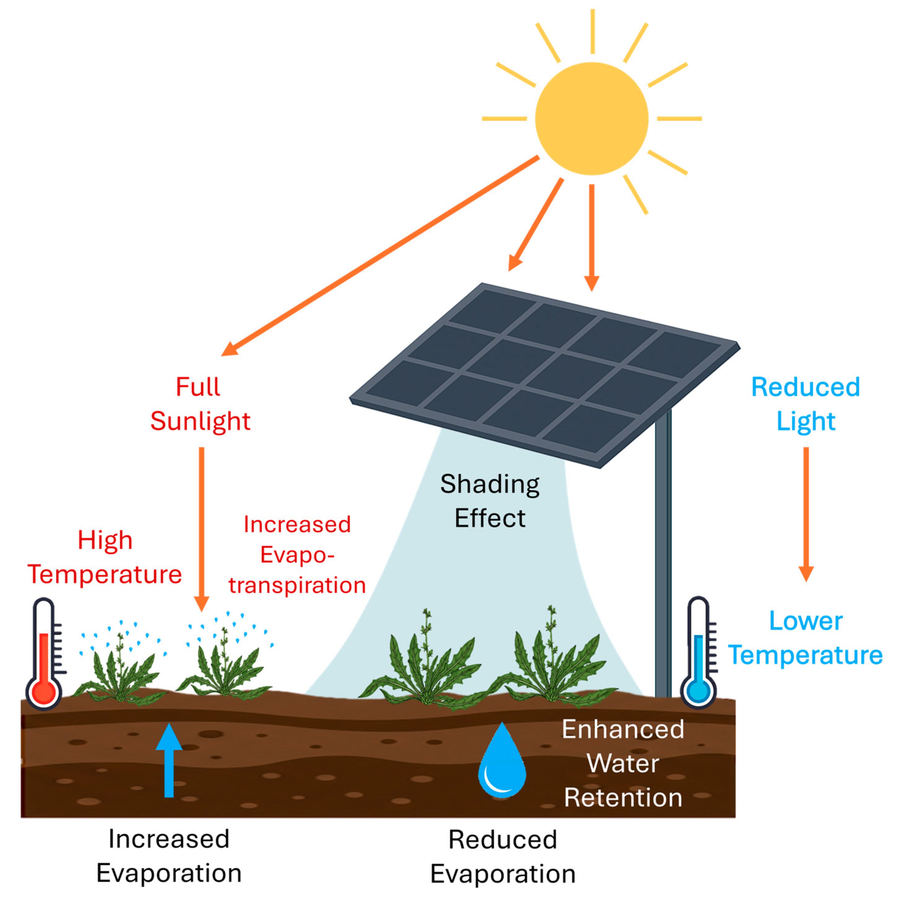
Integrating PV panels in agricultural environments benefits food security by increasing crop yield [1,34,35,36,37,38]. Key findings highlight the environmental benefits of agrivoltaics systems, including reduced greenhouse gas emissions, improved water efficiency, and improved soil quality [39]. Water efficiency is primarily driven by reduced water consumption, which appears to be influenced by evaporation. Mainly, the attenuation of sunlight reaching the soil surface can help reduce water loss and the risk of desertification (Figure 1). As a result, frequent droughts and intense solar radiation can be reduced [1,37,40,41,42].

Figure 1.
Schematic representation of the interaction between photovoltaic panels and crop growth in an agrivoltaic system. The diagram illustrates how shading affects light availability, temperature regulation, and water retention. Plants under full sunlight experience higher temperatures and increased evapotranspiration, leading to greater water loss. In contrast, shaded plants benefit from lower temperatures, reduced light exposure, and enhanced water retention, mitigating water stress and potentially improving biomass production.
This research aims to assess agrivoltaics’ role in enhancing food security by boosting biomass production while maintaining the quality of edible crops, with a focus on minimizing water consumption relative to annual water availability. While the positive effects of agrivoltaics on crop production in drought and heat stress conditions are well-documented, its effectiveness under other weather conditions is less explored [1,34,35,37,39]. This study focuses on chicory, which has shown increased productivity under shaded conditions during drought periods in late spring [1]. This research extends the study to cooler periods, examining chicory’s performance from late winter to early spring to evaluate agrivoltaics’ influence in less water-stressed conditions.
The goal of this study is to evaluate how agrivoltaics impacts food security across varying water availability scenarios by comparing crop production in open-field control plots with that in shaded plots. Crop productivity was assessed by measuring the weight of edible biomass, while quality was evaluated based on pigment concentrations under different light and water conditions. We also investigated the relationship between crop production and abiotic variables such as atmosphere, soil temperature, and moisture. Furthermore, we analyzed water precipitation carrying capacity during the final decade of the study period to determine the optimal water requirements for crop production under different conditions, including areas under PV panels.
2. Materials and Methods
This study is explanatory experimental research aimed at investigating the effects of different light and water regimes on the biomass production of Cichorium intybus L. (variety Otrantina). The experiment was carried out in an open field setting under two distinct environmental conditions: full sunlight and shade, to assess plant responses under agrivoltaic panels. In both conditions, plants were exposed to uncontrolled environmental variables, but key abiotic factors such as air temperature, humidity, soil temperature, moisture, light intensity, and water regimes were monitored to analyze their impact on biomass production.
2.1. Experimental Setup and Techniques
Research followed a hypothetical–deductive methodology to test the hypothesis that shade generated by agrivoltaic systems positively influences chicory growth in cooler weather with varying water availability, as suggested by the prior literature [1]. Hypotheses were tested under controlled sunlight exposure and water regimes to ensure data reliability and validity.
The experimental activities were carried out at the University of Salento’s Botanical Garden, located il Lecce, Apulia, Southern Italy (40°20′08.3″ N 18°07′21.2″ E), from 1 March to 15 April 2024.
Cichorium intybus L. (Otrantina variety) certified seeds were obtained from the University’s Botanical Garden. The seeds were soaked in running tap water for 2–3 h before being sown in 4.5 L plastic pots, with one seed per pot. Each pot was filled with commercial soil and placed in a growth chamber at 22 °C, 60% humidity, 25 μE light intensity, and a 16/8 h photoperiod for seed germination. Irrigation was applied at 100 mL per pot every two days for 45 days [1]. Afterward, the seedlings were transferred to the open field.
The experimental design included two plots: one exposed to full sunlight (L) and the other shaded (S) by a photovoltaic panel (1.4 m × 2.4 m), positioned 2.10 m above the soil to simulate an agrivoltaic system. This setup adhered to Italian agrivoltaic guidelines [43,44], with the panel oriented from northeast to southwest to replicate the typical PV panel orientation in the surrounding area [1,42].
Within each plot, plants were divided into two groups, each consisting of nine chicory plants, subjected to different water regimes: high water regime (HWR) and low water regime (LWR). Irrigation was manually applied, with 400 mL of water per plant every two days for HWR and 200 mL per plant for LWR. Water amounts were measured using a graduated cylinder to ensure accuracy (Table 1). The total water supply was 5.0 L for LWR and 9.4 L for HWR.

Table 1.
Summary of the experimental design characterized by two plots with different sun exposure, and each other characterized by two groups with high water regime (HWR) and low water regime (LWR) [1].
For each plot, daily minimum and maximum air temperatures were recorded using two external thermometers (ThermoPro TP357, Atlanta, GA, USA with an accuracy of ±0.5 °C and measurement range from −20 °C to +60 °C), located one under the shade panel and one in the controlled area, both at the same height from the ground (1 m). Soil temperature and moisture were measured during the hottest day to estimate average conditions for each group (HWR-L, LWR-L, HWR-S, and LWR-S). Additionally, annual precipitation data from 2011 to 2024 were extrapolated from the Apulian Civil Protection Meteorological Stations in Lecce [45].
2.2. Quantitative and Qualitative Evaluation of Chicory Biomass Production
Biomass production was assessed by measuring the fresh weight (fw) and dry weight (dw) of chicory leaves. The basal rosette leaves, representing edible biomass, were harvested, weighed immediately for fw using a precision balance (Mettler Toledo PC 440, Columbus, OH, USA) and photographed for morphological analysis. Leaf morphometry (e.g., major and minor axes, area, and circularity) was analyzed using ImageJ 1.53e software following established protocols [46].
To determine dw, 250 mg of leaf tissue was dried at 60 °C for one week, or until the biomass weight stabilized. The water content of chicory leaves was calculated as the difference between fw and dw [1].
To assess food quality in terms of water stress, chlorophyll (a, b, total) and carotenoid concentrations were determined spectrophotometrically using a Shimadzu® UV-2600 instrument (Kyoto, Japan), following Lichtenthaler and Buschmann’s methods [47]. Results were expressed as nmol/g fw [46].
2.3. Data Interpretation and Statistical Analysis
The hypothesis that shade-grown plants exhibit higher productivity was tested by comparing biomass production under different light and irrigation conditions. Significant differences in fresh and dry biomass production between plants grown in full sunlight and those grown in shade were analyzed. The relationship between biomass production and abiotic environmental variables was also assessed.
Statistical significance was determined by one-way ANOVA to compare the means of each group. Assumptions of normality and homogeneity of variance were checked using the Shapiro–Wilk test (p > 0.05 for normality) and Levene’s test (p > 0.05 for homogeneity) [48,49,50,51,52]. If ANOVA indicated significant differences (p < 0.05), post hoc pairwise comparisons were conducted using Tukey’s Honestly Significant Difference (HSD) test [53].
To examine temperature variations over time, ANCOVA (Analysis of Covariance) was applied to verify the homogeneity of regression slopes [54,55]. If the slopes differed significantly (p < 0.05), the null hypothesis of equal means between groups was rejected.
3. Results
3.1. Biomass Analysis
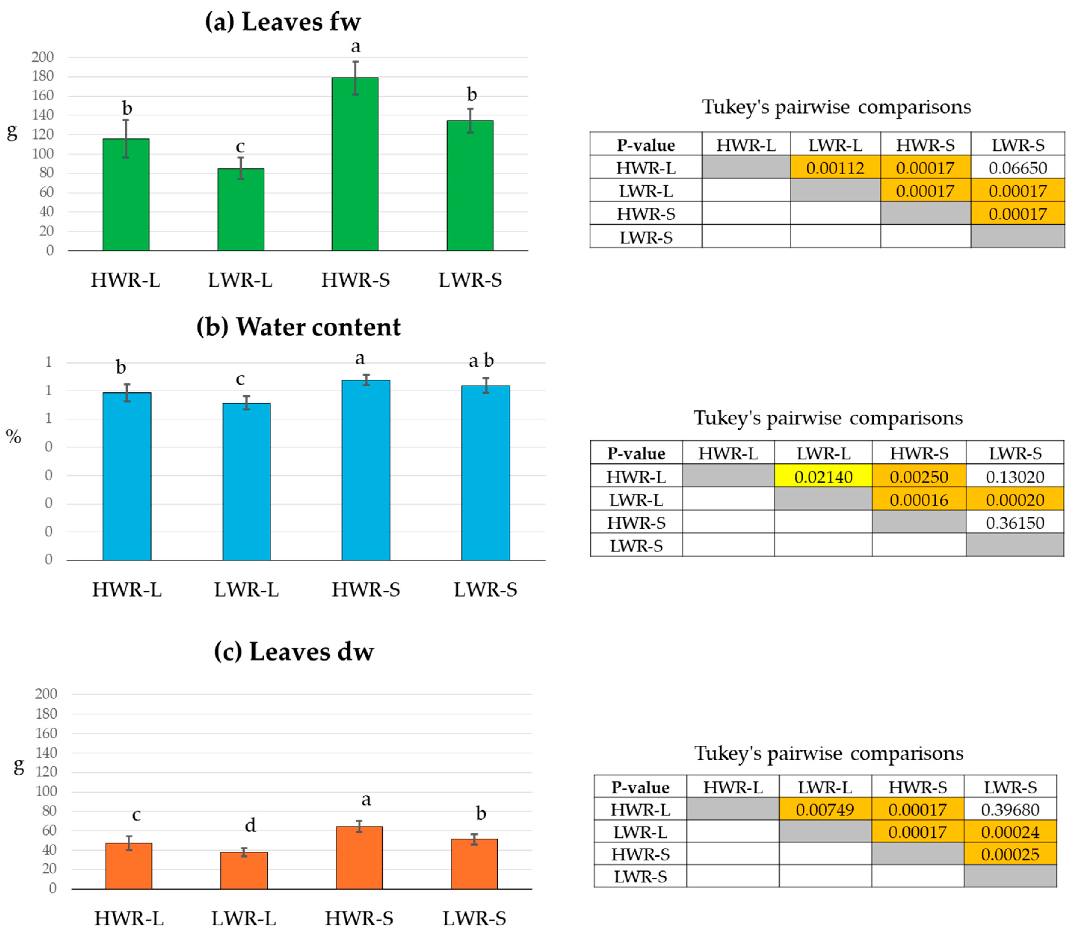
Chicory plant biomass was evaluated under different light and water conditions by measuring fw, dw, and total leaf surface area. Measurements were taken for plants grown in full sunlight (L) or under PV panel shade (S), with exposure to either high (HWR) or low (LWR) water regimes. The average of leaves fw was higher in shaded groups compared to those in full sunlight, and more pronounced under high water regimes than low water regimes (Figure 2a). The one-way ANOVA revealed highly significant differences between the groups under different light conditions (sum of squares 41,463.6; df 3; mean square 13,821.2; F 58.54; p-value: 4.33 × 10⁻¹³). The highest leaves fw was recorded in the HWR-S group (178.9 ± 5.6 g), while the lowest value was found in the LWR-L group (85.2 ± 3.9 g). Although the LWR-S group (134.5 ± 4.2 g) had a higher fw than the HWR-L one (115.0 ± 6.5 g), Tukey’s pairwise comparisons indicated no statistically significant differences between these two groups (Figure 2a).

Figure 2.
Leaves fresh weight (fw) (a), leaves water content (b), and leaves dry weight (dw) (c) of chicory plants grown in full sunlight (L) or under shade (S), subjected to high (HWR) or low (LWR) water regimes. Tukey’s pairwise comparisons are presented in the tables with p-values above the diagonal. Statistically significant differences (p < 0.05) are highlighted with a yellow box and high significant differences (p < 0.001) with an orange box. Uncolored boxes indicate no statistically significant differences. HWR-L: high water regime in sunlight; LWR-L: low water regime in sunlight; HWR-S: high water regime in shade; LWR-S: low water regime in shade. Bars marked in the plot with different letters indicate significant differences among samples (Tukey’s post hoc test, p < 0.05).
Leaves water content was also higher in shade groups (Figure 2b). The one-way ANOVA showed significant differences between the water regimes (sum of squares 334.8; df 3; mean square 111.6; F 18.3; p-value: 4.26 × 10⁻⁷). The HWR-S group had the highest water content (64%), followed by LWR-S (62%). In contrast, the HWR-L and LWE-L had lower values (56% and 54%, respectively). However, Tukey’s test showed that LWR-S did not differ significantly from HWR-L or LWR-S groups (Figure 2b).
Similarly, the leaves dw followed the same trend as leaves fw, with the highest value in the HWR-S group (64.6 ± 5.8 g) and the lowest in LWR-L (37.6 ± 4.2 g) (Figure 2c). One-way ANOVA confirmed significant differences between the groups (sum of sq 3404.65; df 3; mean square 1134.88, F 35.34 and p-value 2.85 × 10⁻¹⁰). However, Tukey’s test revealed no significant difference between HWR-L (46.9 ± 7.1 g) and LWR-S (51.2 ± 5.1 g) (Figure 2c).
Similarly, the leaf dw followed the same trend as fw, with the highest value in the HWR-S group (64.6 g ± 5.8 g) and the lowest in LWR-L (37.6 ± 4.2 g) (Figure 2c). One-way ANOVA confirmed significant differences between the groups (sum of squares = 3404.65; df = 3; mean square = 1134.88; F = 35.34; p-value = 2.85 × 10⁻¹⁰). Tukey’s test revealed no significant difference between HWR-L (46.9 ± 7.1 g) and LWR-S (51.2 ± 5.1 g) (Figure 2c).
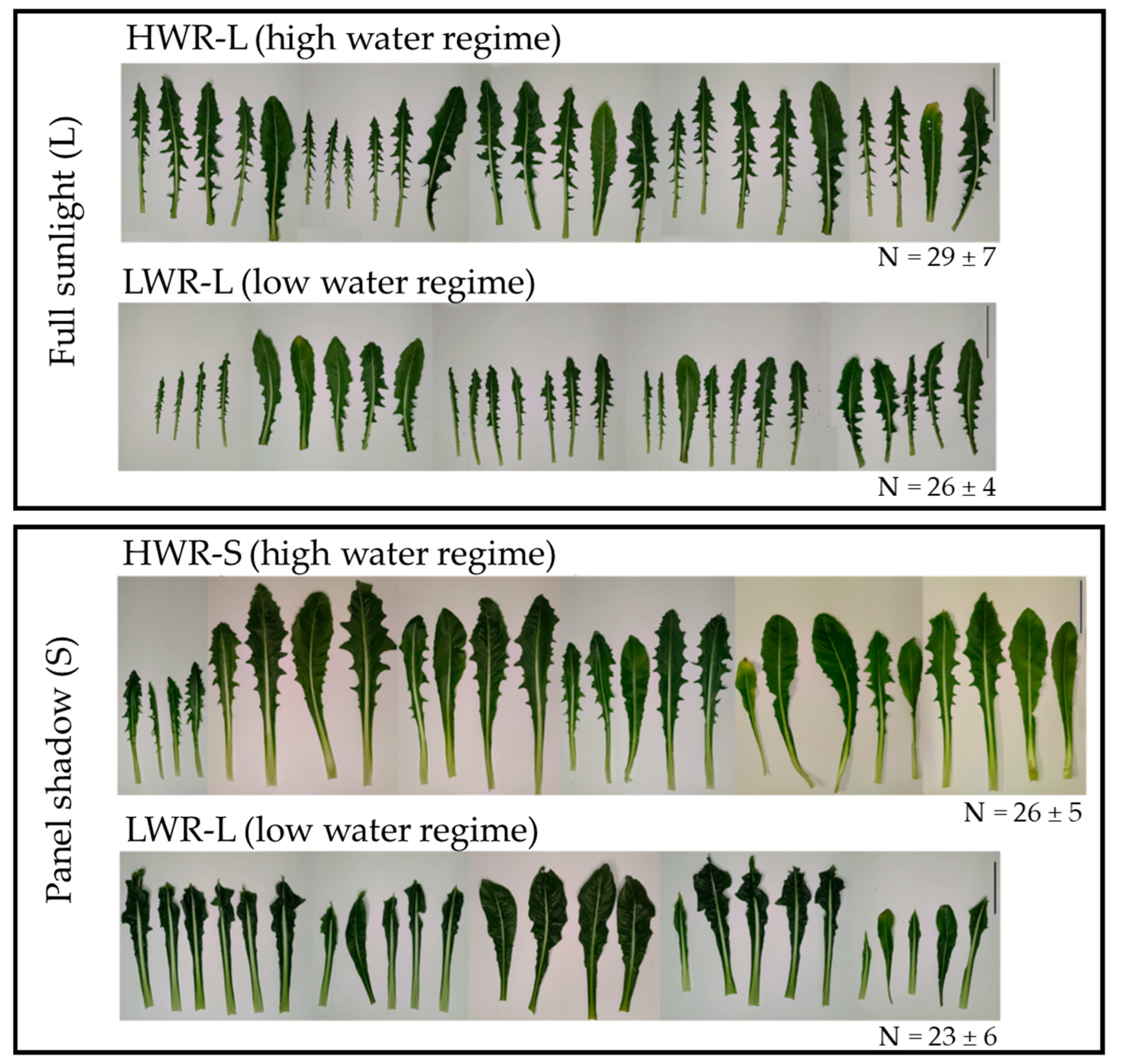
Morphological observations revealed no significant differences in the number of leaves among 45-day-old chicory plants across the groups (HWR-L = 29 ± 7; LWR-L = 26 ± 4; HWR-S = 26 ± 5 and LWR-S = 23 ± 6; ANOVA test: df = 3/32; F = 2.019 and p-value = 0.1267). None of the plants exhibited signs of stress, such as leaf wilting. However, noticeable differences in leaf size and shape were observed, indicating varying responses to different growth conditions (Figure 3). Leaves from plants grown in HWR-L were predominantly oblanceolate with toothed margins, a feature consistent across plants grown in full sunlight regardless of water regime, as well as by HWR-S plants. In contrast, plants grown in shade with limited water (LWR-S) displayed irregular leaf margins. Corroborating this, leaf circularity, calculated as 4 × π × area/perimeter2, differed significantly between groups, with leaves from shaded plants showing higher circularity values (0.23 ± 0.04 for HWR-S and 0.17 ± 0.02 for LWR-S) compared to those grown in sunlight (0.15 ± 0.02 for HWR-L and 0.11 ± 0.02 for LWR-L) (Figure 4a).
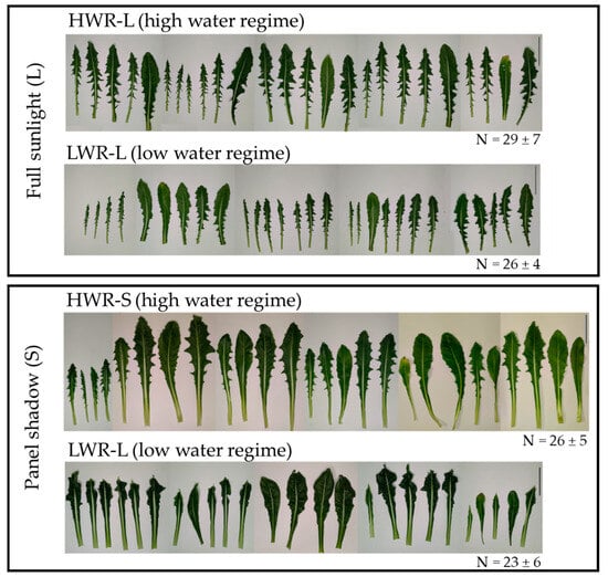
Figure 3.
Leaves morphology of chicory plants from HWR-L, LWR-L, HWR-S and LWR-S groups. N indicates the mean ± the standard deviation of the number of leaves present on each plant grown in the different groups of three independent experiments. HWR-L: high water regime in sunlight; LWR-L: low water regime in sunlight; HWR-S: high water regime in shade; LWR-S: low water regime in shade. Scale bars: 5 cm.
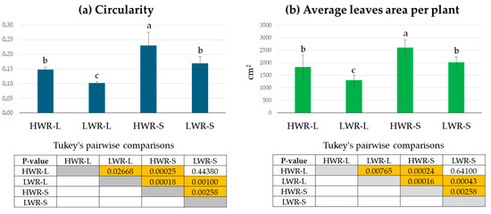
Figure 4.
Leaves circularity values per plant (a) and average leaves area per plant (b) from HWR-L, LWR-L, HWR-S, and LWR-S groups. Tukey’s comparisons: yellow boxes indicate statistically significant differences (p < 0.05), and orange boxes indicate highly significant differences (p < 0.001). Box without color indicates no statistically significant differences. HWR-L: high water regime in sunlight; LWR-L: low water regime in sunlight; HWR-S: high water regime in shade; LWR-S: low water regime in shade. Bars marked in the plot with different letters indicate significant differences among samples (Tukey’s post hoc test, p < 0.05).
Average leaf area was also affected by growing conditions, with the largest leaves (2609 ± 307 cm2) found in HWR-S plants, followed by LWR-S and HWR-L (2014 ± 217 cm2 and 1833.4 ± 481.1 cm2, respectively). The smallest leaves (1302.1 ± 213.9 cm2) were found in the LWR-L group. While ANOVA indicated significant differences among groups (df = 3/32; F = 24.95; p-value = 1.61 × 10⁻⁸), pairwise comparisons showed no significant difference between HWR-L and LWR-S but supported the ANOVA results in the other cases (Figure 4).
3.2. Chlorophyll and Carotenoid Content
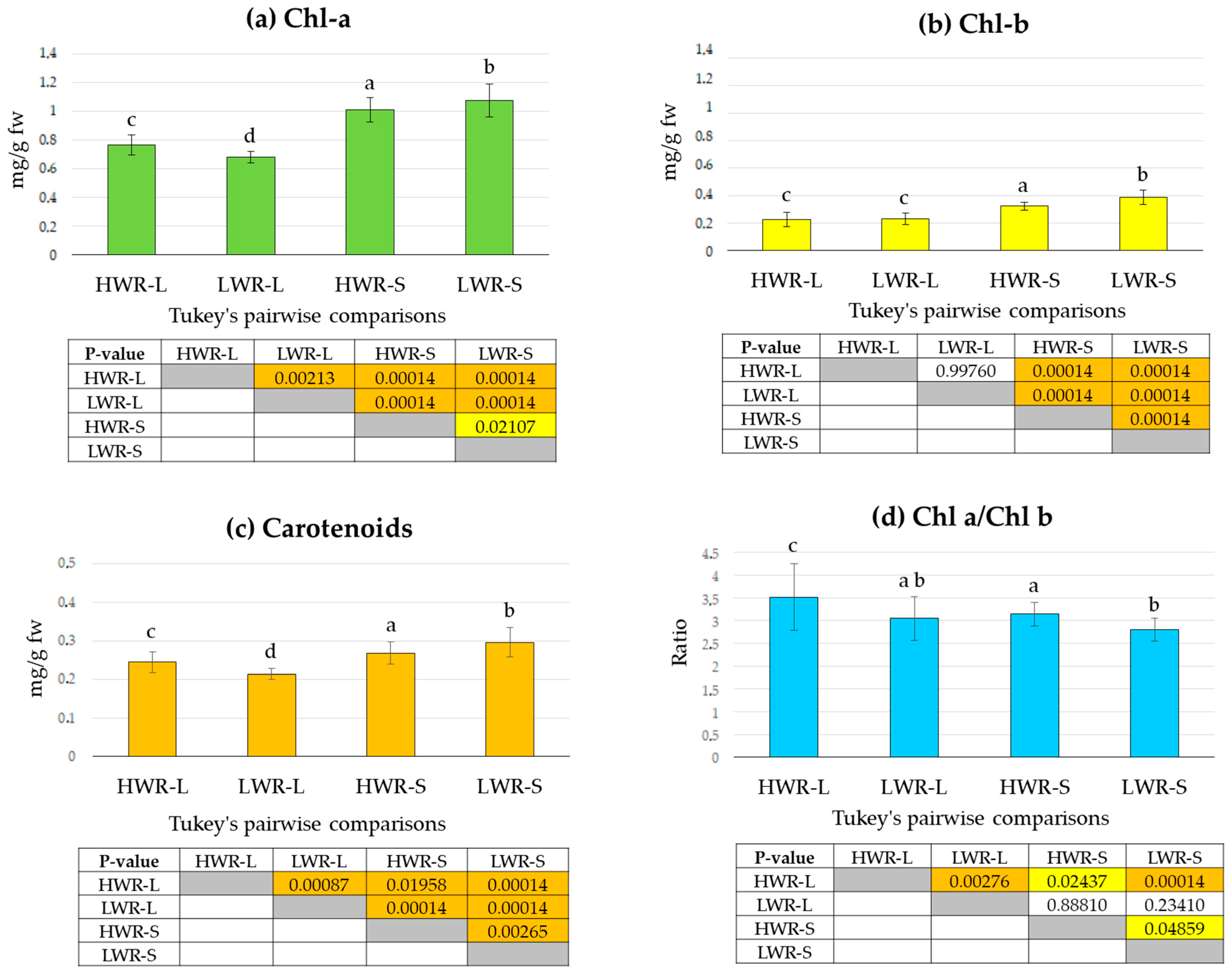
Wavelengths of light and water stress can significantly influence photosynthetic activity, thereby affecting chlorophyll and carotenoid content [56,57]. To investigate the effects of shade and varying irrigation regimes under our experimental conditions, we quantified chlorophyll and carotenoid content across the four treatment groups. Pigment analysis revealed that levels of chlorophyll a (Chl a, Figure 5a), chlorophyll b (Chl, Figure 5b), and carotenoids (Figure 5c) were highest in the LWR-S group (Chl a: 1.08 ± 0.11 mg/g fw, Chl b: 0.39 ± 0.05 mg/g fw and carotenoids: 0.30 ± 0.05 mg/g fw), followed by the HWR-S group (Chl a: 1.01 ± 0.08 mg/g fw, Chl b: 0.32 ± 0.04 mg/g fw and carotenoids: 0.28 ± 0.03 mg/g fw), both of which were grown in shaded conditions. In contrast, lower pigment concentrations were obtained in the LWR-L (Chl a: 0.67 ± 0.07 mg/g fw, Chl b: 0.23 ± 0.04 mg/g fw, and carotenoids: 0.21 ± 0.01 mg/g fw) and HWR-L (Chl a: 0.76 ± 0.07 mg/g fw, Chl b: 0.23 ± 0.05 mg/g fw and carotenoids 0.24 ± 0.03 mg/g fw) groups, which were grown under full sunlight. One-way ANOVA revealed statistically significant differences among the groups for Chl a (df = 3/32, F = 142.9, p = 9.461 × 10−37), Chl b (df = 3/32 F = 78.44, p = 1.348 × 10⁻²⁶). and carotenoids levels (df = 3/32, F = 40.0, p = 2.82 × 10⁻¹⁷). However, Tukey’s pairwise comparisons indicated no statistically significant differences in Chl b levels between the two full sunlight groups (HWR-L and LWR-L), while supporting the ANOVA results for the other comparisons. The ratio of Chl a to Chl b was highest in the HWR-L group, followed by the HWR-S, both characterized by a higher water regime (Figure 5d), lower ratios were instead observed in the LWR-S and LWR-L plots. One-way ANOVA showed statistically significant differences in the Chl a/Chl b ratio among the groups (df = 3/32, F = 10.4, p = 4.59 × 10⁻⁶), though Tukey’s pairwise comparisons did not show statistically significant differences between LWR-L group and the HWR-S or LWR-S groups.
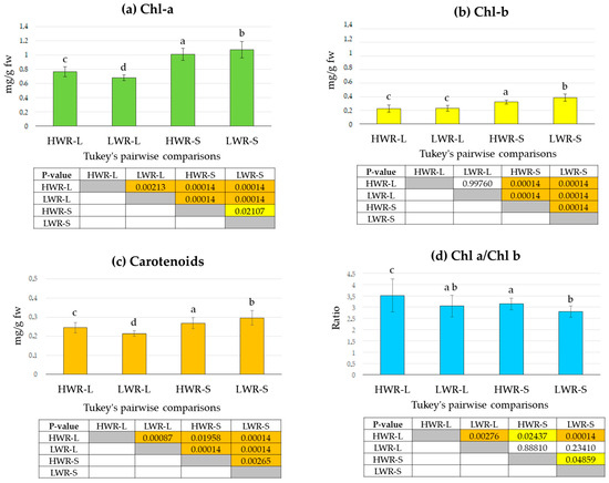
Figure 5.
Chlorophyll a (a), chlorophyll b (b), and carotenoids (c) contents, and the Chl a/Chl b ratio (d) in chicory leaves from the HWR-L, LWR-L, HWR-S and LWR-S groups. In the tables, yellow boxes indicate statistically significant differences (p < 0.05), orange boxes indicate high statistically significant differences (p < 0.001), and uncolored boxes indicate no statistically significant differences. HWR-L: high water regime in sunlight; LWR-L: low water regime in sunlight; HWR-S: high water regime in shade; LWR-S: low water regime in shade. Bars marked in the plot with different letters indicate significant differences among samples (Tukey’s post hoc test, p < 0.05).
3.3. Abiotic Variables Analysis
Maximum temperatures in the two experimental plots (full sunlight and shade) increased over time, with statistically significant differences between the groups (ANCOVA, F = 6.733, p = 0.011; homogeneity of slopes: F = 1.13. p = 0.291; residual normality tested with Shapiro–Wilk). Maximum air temperatures were consistently higher in the full sunlight plot, with differences of up to 10 °C compared to the shaded plot. However, minimum air temperatures did not show statistically significant differences between the groups (ANCOVA, F = 2.444, p = 0.138; homogeneity of slopes: F = 0.004, p = 0.949; residual normality tested with Shapiro–Wilk) (Figure 6).
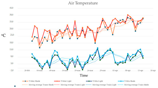
Figure 6.
Maximum and minimum air temperatures recorded in the full sunlight plots (HWR-L and LWR-L) and shaded plots under the PV panels (HWR-S and LWR-S) from 1 March 2024, to 15 April 2024. Dotted lines indicated the linear trends over time.
Moreover, no significant differences in maximum or minimum air humidity were found between full sunlight and shade plots. Maximum air humidity remained around 99% for both plots, with only minor variations (Figure 6). Minimum air humidity was higher under the shade, but this difference was not statistically significant (ANCOVA, F = 1.68, p = 0.198; homogeneity of slopes: F = 0.004, p = 0.949; residual normality tested with Shapiro–Wilk) (Figure 7).
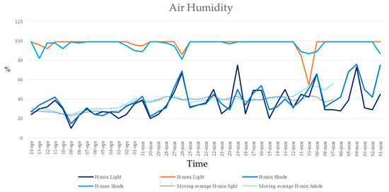
Figure 7.
Minimum and maximum air humidity recorded in the full sunlight plots (HWR-L and LWR-L) and shaded plots under the PV panels (HWR-S and LWR-S) from 1 March 2024 to 15 April 2024. Dotted lines indicated the linear trends over time.
Illuminance values recorded during maximum shade under the panels were approximately 4136 ± 693 lx, while full sunlight values reached around 128,341 ± 7165 lx. These values were highly significantly different (t-test, p = 9.1 × 10⁻⁹). ANOVA revealed that watering regime, illuminance, and air temperature significantly affected soil temperature (sum of squares 1848.9, df = 3/32, mean square = 616.3, F = 25.1, p = 1.9 × 10⁻¹⁴) (Figure 8a) and soil moisture (sum of squares 3595.3, df = 3/32; mean square = 1198.4, F = 61.9, p = 8.4 × 10⁻³¹) (Figure 8b). Shaded plots showed lower average soil temperatures (HWR-S: 20.6 ± 4.2 °C and LWR-S: 25.0 ± 5.3 °C) compared to full sunlight plots (HWR-L: 27.7 ± 5.6 °C and LWR-L: 28.5 ± 4.6 °C). Pairwise comparisons showed no significant differences in soil temperature between the full sunlight groups (HWR-L vs. LWR-L) or the shaded groups (HWR-S vs. LWR-S). Soil moisture was higher in the HWR-S (22.9 ± 4.8%) and HWR-L (22.2 ± 4.1%) groups, both receiving a high-water regime, compared to the LWR-S (13.9 ± 3.7%) and LWR-L (20.2 ± 4.9%) groups, which received less water. Pairwise comparisons indicated no statistically significant differences in soil moisture between the high-water regime groups (HWR-L vs. HWR-S).
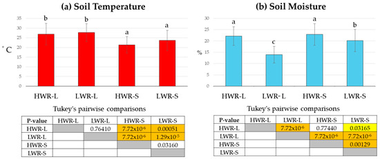
Figure 8.
Average soil temperature (a) and moisture (b) for chicory plants (9 plants per plot) grown in full sunlight and shade under PV panels, subjected to different water regimes. Tukey’s pairwise comparisons are shown in tables: Q values below the diagonal, p-values (same) above. Yellow boxes indicate0 statistically significant differences (p < 0.05), orange boxes indicate highly significant differences (p < 0.001), and uncolored boxes indicate no significant differences. Bars marked in the plot with different letters indicate significant differences among samples (Tukey’s post hoc test, p < 0.05).
The annual cumulative precipitation showed strong variability, consistently remaining below 900 mm. Between 1 January and 30 April, precipitation was always below 400 mm, and in the chicory cultivation period (1 February to 30 April), it remained under 200 mm (Figure 9).
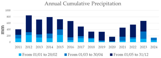
Figure 9.
Annual cumulative precipitation from January 2011 to June 2024, as recorded by the Apulian Civil Protection meteorological stations in Lecce. The dates shown in the title of the graph indicate the day and month when the information was aggregated for each year, and are highlighted in different colours in the graph.
Annual cumulative precipitation showed strong variability, consistently remaining below 900 mm. Between January 1 and April 30, precipitation was always below 400 mm, and during the chicory cultivation period (1 February to 30 April), it remained under 200 mm (Figure 9).
4. Discussion
4.1. Biomass Production and Water Saving
Agriculture is increasingly threatened by the dual challenges of climate change, which leads to reduced water availability and higher temperatures [13,58,59]. Additionally, competition for land use is intensifying as PV farms expand for renewable energy production, driven by policies aimed at reducing carbon dioxide emissions [13].
Our study demonstrates that integrating crop cultivation with PV installations, referred to as agrivoltaics, can effectively support food security by improving biomass production even in the face of climate change pressures. While previous studies have focused on biomass production during hotter months (e.g., May and June) [1,36], fewer have explored the impacts of agroecological practices during cooler periods [60,61].
In this study, chicory plants grown in shaded conditions beneath PV panels exhibited a 41% increase in biomass production compared to full sunlight conditions with the same HWR. Similarly, shaded plants in the low watered regime (LWR) group produced 46% more biomass than their full sunlight counterparts. Remarkably, biomass production in the LWR-S group was statistically comparable to that of the HWR-L group, despite receiving 50% less water.
Our findings align with previous research that observed higher biomass production in shaded environments compared to full sunlight, even during different seasons characterized by higher temperatures and light intensities [1]. Both experiments were conducted at the same location and employed similar cultivation and biomass measurement methods, with the primary difference being the season of cultivation.
In the present study, conducted in late winter and early spring, the mean maximum temperature in the full sunlight area was 29.2 ± 1.6 °C, while in the shaded area under the panels, it was 26.9 ± 3.7 °C. In contrast, the previous experiment carried out between late spring and early summer, recorded a mean maximum temperature of 38.1 ± 5.4 °C in full sunlight and 33.9 ± 2.7 °C in the shaded area.
Illuminance levels also varied between the two studies. In the present experiment, the maximum illuminance under the panels was approximately 4136 ± 693 lx, while in full sunlight, it reached 128,341 ± 7165 lx. In the previous experiment, illuminance under the panels was 9388 ± 1339 lx, compared to 166,485 ± 13,037 lx in full sunlight [1].
Despite these differences in temperature and solar radiation, both studies consistently demonstrated that the shading provided by the agrivoltaic system enhances biomass production compared to full sunlight conditions.
These findings demonstrate that agrivoltaics can efficiently support food production while saving water, regardless of the crop’s primary growing season (spring and summer), making it a promising strategy for agricultural sustainability, especially in water-limited regions. The agricultural productivity of an agrivoltaic system is primarily determined by the PV panel technology and configuration, which includes row spacing and overall layout [62].
In the context of the Apulia region, Southern Italy, water-saving strategies like agrivoltaics could significantly reduce irrigation costs for crops such as chicory. Currently, the cost of chicory production, based on water usage, could drop from a range of EUR 125–325/ha to EUR 725–2175/ha, depending on water prices (ranging from EUR 0.25/m3 to EUR 1.45/m3) and crop water needs of water in consideration of climate conditions (1000–3000 m3/ha) [63]. These findings are particularly relevant given the region’s low annual rainfall, which has stayed below 900 mm over the past 12 years (2011–2023), with less than 200 mm recorded during the chicory growing season (February–April) (Figure 8). Water saving is critical in Southern Italy where rainfall is insufficient to meet the water demand for crop production. The availability of water for agriculture, human use, and ecosystems largely depends on the spatial and temporal distribution of precipitations and on evapotranspiration rates [64,65,66]. Chicory’s water requirements exceed the region’s natural precipitation, resulting in a consistent water deficit. To address this challenge, it is essential to implement rainwater harvesting systems that maximize the use of available rainfall, promoting sustainable crop production despite limited water resources.
As water resources become limited due to climate change, enhancing soil water retention will be critical for food security. Projections indicate that temperate regions will face increasing water stress in the coming years [58]. Therefore, agrivoltaics offers a viable solution to mitigate water shortages by maintaining crop yields under reduced water availability, highlighting its potential to contribute to global food security efforts.
4.2. Differences in Photosynthetic Pigment Concentrations
Plants growing in full sunlight underwent more severe water stress than those under PV panels, which negatively affects chlorophyll (Chl a and Chl b) concentrations. Water stress accelerates oxidative processes that degrade chlorophylls, reducing the plant’s capacity to absorb light and impairing photosynthetic carbon fixation processes [67]. This study showed that plants grown in full sunlight had lower chlorophyll concentrations than those grown in shaded conditions, regardless of water regime (Figure 8). This reduced chlorophyll content likely compromises photosynthetic efficiency, resulting in lower biomass production in sun-exposed plots.
Chlorophyll content is a well-established indicator of photosynthetic capacity, supported by strong physiological and biochemical evidence. A significant correlation exists between leaf chlorophyll content and maximum carboxylation capacity, which regulates the maximum rate of CO2 assimilation. Since chlorophyll is responsible for light capture, it directly influences the energy available for the Calvin–Benson cycle reactions [68].
The ratio of Chl a to Chl b also varied across groups, reflecting the plants’ adaptative responses to light intensity. Plants in high-light environments, such as those in full sunlight, typically exhibit higher Chl a/Chl b ratios, explaining the differences observed between HWR-L and HWR-S groups. Instead, in shaded conditions, the lower Chl a/Chl b ratio may suggest that the plant requires more Chl b to absorb the available light. Under water stress, however, there can be a relative increase in Chl b compared to Chl a, as Chl b may be more resilient to environmental stress [1,69,70,71]. This trend explains the differences between the HWR and LWR groups under both light conditions.
Despite a lower Chl a/Chl b ratio in shaded plants, the concentrations of both Chl a and Chl b are higher compared to plants grown in full sunlight. Additionally, shaded plants accumulate more biomass (both fresh and dry), which reflects the organic matter produced and serves as a growth index. This suggests that the plants are better adapted to the limited light conditions under the panels, likely supporting enhanced growth despite reduced light intensity [71,72].
Higher carotenoid concentrations were also observed in plants grown under the PV panels, likely due to their ability to adjust to low-light conditions. Indeed, carotenoids are crucial for absorbing blue–green light, which predominates in shaded environments [1].
4.3. The Impact of Abiotic Components
Biomass production and pigment concentrations were influenced not only by irrigation but also by differences in light intensity and temperature between the full sunlight and shaded plots. In this study, light levels (illuminance values) in the shade plot were only 3% of those in the full sunlight plots during midday (11:00–14:00), which contributed to lower soil and air temperatures. Maximum air temperature in full sunlight was up to 10 °C higher than in shaded pots, likely explaining the increased water stress experienced by plants in sun-exposed areas (Figure 2).
Soil moisture levels did not differ significantly between the HWR-L and HWR-S groups, but the average soil temperature was notably higher in the full sunlight plots (Figure 8). This pattern was consistent across the LWR groups. No significant temperature differences were observed between LWR-L and HWR-L; however, a significant difference in soil moisture was detected, reflecting the varying water regimes between the two groups. A similar trend was recorded in the shaded plot, where soil moisture differed significantly between LWR-S and HWR-S, but no significant temperature differences were found.
Unlike many studies that attribute enhanced crop yields under PV panels primarily to differences in soil moisture compared to fully sunlight conditions [1], our findings suggest that the key driver of biomass production is the reduction in both soil and air temperature afforded by the PV panels, rather than soil moisture levels alone. This temperature modulation appears to play a more significant role in promoting plant growth and productivity under shaded conditions.
Agrivoltaics’ ability to mitigate temperature stress is particularly relevant in light of the global temperature anomaly trends observed since 1989. European countries have experienced even higher temperature anomalies compared to the global average, with peaks of 3 °C above normal, compared to 2 °C globally (Figure 10). By reducing maximum temperatures by up to 10 °C, PV panels can help mitigate the adverse effects of rising temperatures on crop production.
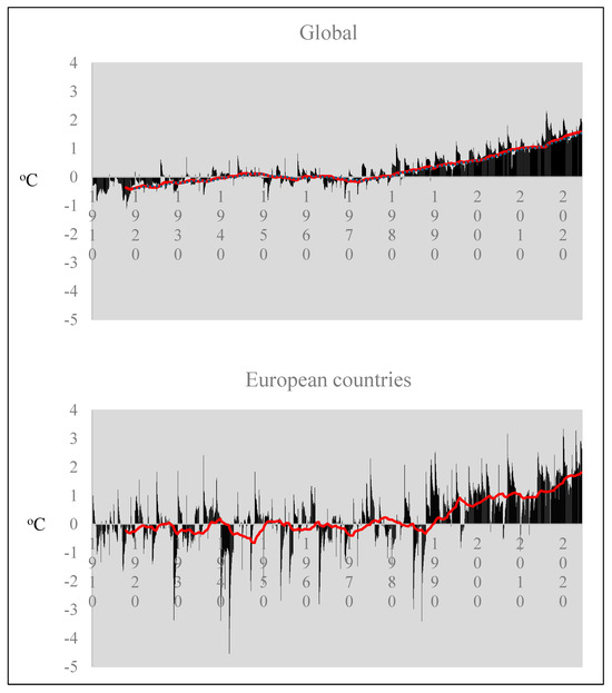
Figure 10.
Monthly average temperature anomalies on global and European scales. The red line represents the moving average of values over time [73] (Annual Global Climate Report, 2024).
5. Conclusions
Many studies have demonstrated the benefits of agrivoltaic systems in supporting crop production during hot periods, primarily by maintaining higher soil moisture levels under PV panels compared to full sunlight conditions. However, this study reveals that agrivoltaics can also enhance food production during favorable weather conditions for crop growth, as observed in this case study conducted from March to April 2024. By growing chicory under identical soil and irrigation conditions (both high and low water regimes), we observed that the increased crop yield under PV panels was not related to soil moisture retention but to reduced water stress, as the shaded plants experienced lower soil and air temperatures compared to those in full sunlight. This reduction in water stress was confirmed by photosynthetic pigment analysis (Chl a, Chl b, and carotenoids), which indicated better physiological performance under the PV panels.
The results of this study show that efficiency in water use can be linked to a direct reduction in water stress on plants and less on soil evapotranspiration. Thus, agrivoltaics helps to reduce the water footprint of agricultural activities by supporting crop production with lower water inputs, without sacrificing biomass yield compared to traditional farming systems. This reduction in water use also lowers production costs while maintaining food output, making agrivoltaics particularly valuable in the context of global warming. The cumulative annual precipitation data further emphasize the importance of water saving, as crop activities frequently operate at a water deficit, using more water than is replenished by annual rainfall. The main limitation of this study is that the experiments focused on a single variety and a single growing season. Given the different seasons in which chicory can be grown, it would be valuable to apply the same methodological analysis to another season that has not yet been tested. Furthermore, it is essential to extend this methodology to fruit crops to assess the different effects of the agrivoltaic system on crop production.
With the global population expected to increase by 70% by 2050 and corresponding demands for both energy and food (United Nations, 2014), agrivoltaics presents an innovative solution within international energy policy to reduce greenhouse gas emissions, which aligns well with strategies such as the Common Agricultural Policy (CAP), which aims to ensure food security while promoting sustainable and environmentally friendly agricultural practices (CAP, 2024).
Author Contributions
Conceptualization, A.S. (Aurelia Scarano), T.S. and M.D.C.; methodology, A.S. (Aurelia Scarano), T.S., L.M.C. and M.D.C.; software, A.S. (Aurelia Scarano), T.S., L.M.C. and M.D.C.; validation, A.S. (Aurelia Scarano), T.S. and M.D.C.; formal analysis, A.S. (Aurelia Scarano), T.S. and M.D.C.; investigation, A.S. (Aurelia Scarano), T.S. and M.D.C.; resources, T.S., M.S.L., A.S. (Angelo Santino), A.B. and M.D.C.; data curation, T.S. and A.C.; A.S. (Aurelia Scarano), L.M.C.; writing—original draft preparation, A.S. (Aurelia Scarano), T.S. and M.D.C.; writing—review and editing, A.S. (Aurelia Scarano), T.S., A.C., L.M.C., M.S.L., A.S. (Angelo Santino), A.B. and M.D.C.; visualization, A.S. (Aurelia Scarano), T.S., A.C., L.M.C., M.S.L., A.S. (Angelo Santino), A.B. and M.D.C.; supervision, T.S., M.S.L., A.S. (Angelo Santino), A.B. and M.D.C.; funding acquisition, M.S.L., A.S. (Angelo Santino), A.B. and M.D.C. All authors have read and agreed to the published version of the manuscript.
Funding
This work was supported by the PRIN 2022-SAPPHIRE (CUP2022MWK7Y7) funded by the European Union—Next Generation EU the Italian Ministry of Research (MUR).
Data Availability Statement
Data is contained within the article.
Acknowledgments
The publication has been funded by EU—Next Generation EU Mission 4 “Education and Research”—Component 2: “From research to business”—Investment 3.1: “Fund for the realisation of an integrated system of research and innovation infrastructures”—Project IR0000032—ITINERIS—Italian Integrated Environmental Research Infrastructures System—CUP B53C22002150006. The authors acknowledge the Research Infrastructures participating in the ITINERIS project with their Italian nodes: ACTRIS, ANAEE, ATLaS, CeTRA, DANUBIUS, DISSCO, e-LTER, ECORD, EMPHASIS, EMSO, EUFAR, Euro-Argo, EuroFleets, Geoscience, IBISBA, ICOS, JERICO, LIFEWATCH, LNS, N/R Laura Bassi, SIOS, SMINO. The authors gratefully acknowledge the financial support for this research, including the PhD scholarship of Lorenzo Maria Curci, provided by the Italian National Recovery and Resilience Plan (PNRR), Mission 4, Component 2, Investment 3.3, as per D.M. n. 352/2022 (CUP F83C22000800006), funded by the European Union—Next GenerationEU. The authors also wish to thank R.I. Group S.p.a., Trepuzzi, Lecce, for their valuable co-funding contribution to this study. Views and opinions expressed are however those of the author(s) only and do not necessarily reflect those of the European Union or the European Commission. Neither the European Union nor the European Commission can be held responsible for them.
Conflicts of Interest
The authors declare no conflicts of interest.
References
- Semeraro, T.; Scarano, A.; Curci, L.M.; Leggieri, A.; Lenucci, M.; Basset, A.; Santino, A.; Piro, G.; De Caroli, M. Shading effects in agrivoltaic systems can make the difference in boosting food security in climate change. Appl. Energy 2024, 358, 122565. [Google Scholar] [CrossRef]
- Diamond, J. Evolution, consequences and future of plant and animal domestication. Nature 2002, 418, 700e707. [Google Scholar] [CrossRef] [PubMed]
- Notarnicola, B.; Sala, S.; Assumpció, A.; McLaren, S.J.; Saouter, E.; Sonesson, U. The role of life cycle assessment in supporting sustainable agri-food systems: A review of the challenges. J. Clean. Prod. 2017, 140, 399–409. [Google Scholar] [CrossRef]
- FAO; IFAD. The State of Food Security and Nutrition in the World: Building Climate Resilience for Food Security and Nutrition. Food and Agriculture Organization of the United Nations. Rome, 2018, FAO. Available online: https://openknowledge.fao.org/server/api/core/bitstreams/f5019ab4-0f6a-47e8-85b9-15473c012d6a/content (accessed on 4 February 2025).
- Mirzabev, A.; Kerr, R.B.; Hasegawa, T.; Pradhan, P.; Wreford, A.; von der Pahlen, M.C.T.; Gurney-Smith, H. Severe climate change risks to food security and nutrition. Clim. Risk Manag. 2023, 39, 100473. [Google Scholar] [CrossRef]
- HLPE. Food Security and Nutrition: Building a Global Narrative Towards 2030. 2020. Available online: https://www.fao.org/3/ca9731en/ca9731en.pdf (accessed on 5 May 2022).
- Tilman, D.; Fargione, J.; Wolff, B.; D’Antonio, C.; Dobson, A.; Howarth, R.; Swackhamer, D. Forecasting agriculturally driven global environmental change. Science 2001, 292, 281–284. [Google Scholar] [CrossRef]
- Garnett, T. Where are the best opportunities for reducing greenhouse gas emissions in the food system (including the food chain)? Food Policy 2011, 36, S23–S32. [Google Scholar] [CrossRef]
- McMichael, A.J.; Powles, J.W.; Butler, C.D.; Uauy, R. Food, livestock production, energy, climate change, and health. Lancet 2007, 370, 1253e1263. [Google Scholar] [CrossRef]
- Toniolo, S.; Russo, I.; Bravo, I. Integrating product-focused life cycle perspectives in the fresh food supply chain: Revealing intra- and inter-organizational views. Sustain. Prod. Consum. 2024, 48, 46–61. [Google Scholar] [CrossRef]
- Mehran, A.; AghaKouchak, A.; Nakhjiri, N.; Stewardson, M.J.; Peel, M.C.; Phillips, T.J.; Wada, Y.; Ravalico, J.K. Compounding Impacts of Human-Induced Water Stress and Climate Change on Water Availability. Sci. Rep. 2017, 7, 6282. [Google Scholar] [CrossRef]
- United Nations. World Population Projected to Reach 9.8 Billion in 2050, and 11.2 Billion in 2100. Department of Economic and Social Affairs. 2024. Available online: https://www.un.org/tr/desa/world-population-projected-reach-98-billion-2050-and-112-billion-2100 (accessed on 4 February 2025).
- Semeraro, T.; Scarano, A.; Leggieri, A.; Calisi, A.; De Caroli, M. Impact of Climate Change on Agroecosystems and Potential Adaptation Strategies. Land 2023, 12, 1117. [Google Scholar] [CrossRef]
- Stian, B.H.; Erling, M. Natural capital in integrated assessment models of climate change. Ecol. Econ. 2015, 116, 354–361. [Google Scholar] [CrossRef]
- Willis, K.J.; Bhagwat, S.A. Biodiversity and climate change. Science 2009, 326, 806–807. [Google Scholar] [CrossRef] [PubMed]
- Filho, W.L.; Nagy, G.J.; Setti, A.F.F.; Sharifi, A.; Donkor, F.K.; Batista, K.; Djekic, I. Handling the impacts of climate change on soil biodiversity. Sci. Total Environ. 2023, 869, 161671. [Google Scholar] [CrossRef] [PubMed]
- Kamboj, R.; Kamboj, S.; Kamboj, S.; Kriplani, P.; Dutt, R.; Guarve, K.; Grewal, A.S.; Srivastav, A.L.; Gautam, S.P. Chapter 1-Climate uncertainties and biodiversity: An overview. In Visualization Techniques for Climate Change with Machine Learning and Artificial Intelligence; Srivastav, A., Dubey, A., Kumar, A., Kumar Narang, S., Ali Khan, M., Eds.; Elsevier: Amsterdam, The Netherlands, 2023; pp. 1–14. ISBN 9780323997140. [Google Scholar] [CrossRef]
- Hopkins, W.G.; Huner, N.P.A. Introduction to Plant Physiology; John Wiley & Sons, Inc.: Hoboken, NJ, USA, 2004; ISBN 978-0-470-24766-2. [Google Scholar]
- Costanza, R.; Fisher, B.; Mulder, K.; Liu, S.; Christopher, T. Biodiversity and ecosystem services: A multi-scale empirical study of the relationship between species richness and net primary production. Ecol. Econ. 2007, 61, 478–491. [Google Scholar] [CrossRef]
- Semeraro, T.; Mastroleo, G.; Pomes, P.; Luvisi, A.; Gissi, E.; Aretano, R. Modelling Fuzzy combination of remote sensing vegetation index for durum wheat crop analysis. Comput. Electron. Agric. 2019, 156, 684–692. [Google Scholar] [CrossRef]
- Semeraro, T.; Luvisi, A.; Lillo, A.; Aretano, R.; Buccolieri, R.; Marwan, N. Recurrence Analysis of Vegetation Indices for Highlighting the Ecosystem Response to Drought Events: An Application to the Amazon Forest. Remote Sens. 2020, 12, 907. [Google Scholar] [CrossRef]
- Lakhiar, I.A.; Yan, H.; Zhang, C.; Zhang, J.; Wang, G.; Deng, S.; Syed, T.N.; Wang, B.; Zhou, R. A review of evapotranspiration estimation methods for climate-smart agriculture tools under a changing climate: Vulnerabilities, consequences, and implications. J. Water Clim. Change 2025, 16, 249–288. [Google Scholar] [CrossRef]
- Lakhiar, I.A.; Yan, H.; Zhang, J.; Wang, G.; Deng, S.; Bao, R.; Zhang, C.; Syed, T.N.; Wang, B.; Zhou, R.; et al. Plastic Pollution in Agriculture as a Threat to Food Security, the Ecosystem, and the Environment: An Overview. Agronomy 2024, 14, 548. [Google Scholar] [CrossRef]
- Mancosu, N.; Snyder, R.L.; Kyriakakis, G.; Spano, D. Water Scarcity and Future Challenges for Food Production. Water 2015, 7, 975–992. [Google Scholar] [CrossRef]
- FAO. World Agriculture, Towards 2030/2050. FAO, Rome. 2006. Available online: http://www.fao.org/fileadmin/user_upload/esag/docs/Interim_report_AT2050web.pdf (accessed on 4 February 2025).
- FAO. Livestock Environmental Assessment and Performance (LEAP) Partnership. 2015. Available online: http://www.fao.org/partnerships/leap/en/ (accessed on 4 February 2025).
- Lakhiar, I.A.; Yan, H.; Zhang, C.; Wang, G.; He, B.; Hao, B.; Han, Y.; Wang, B.; Bao, R.; Syed, T.N.; et al. A Review of Precision Irrigation Water-Saving Technology under Changing Climate for Enhancing Water Use Efficiency, Crop Yield, and Environmental Footprints. Agriculture 2024, 14, 1141. [Google Scholar] [CrossRef]
- Soussana, J.F. Research priorities for sustainable agri-food systems and life––cycle assessment. J. Clean. Prod. 2014, 73, 19e23. [Google Scholar] [CrossRef]
- Dixon, G.R. Chapter 17-The Impact of Climate and Global Change on Crop Production. In Climate Change Observed Impacts on Planet Earth; Letcher, T.M., Ed.; Elsevier: Amsterdam, The Netherlands, 2009; pp. 307–324. [Google Scholar] [CrossRef]
- Habib-ur-Rahman, M.; Ahmad, A.; Raza, A.; Hasnain, M.U.; Alharby, H.F.; Alzahrani, Y.M.; Bamagoos, A.A.; Hakeem, K.R.; Ahmad, S.; Nasim, W.; et al. Impact of climate change on agricultural production; Issues, challenges, and opportunities in Asia. Front. Plant Sci. 2022, 13, 925548. [Google Scholar] [CrossRef]
- Scharff, L.B.; Saltenis, V.L.R.; Jenen, P.E.; Baekelandt, A.; Burgess, A.J.; Burow, M.; Ceriotti, A.; Cohan, J.-P.; Geu-Flores, F.; Halkien, B.A.; et al. Prospects to improve nutritional quality of crops. Food Energy Secur. 2021, 11, e327. [Google Scholar] [CrossRef]
- Wu, J.; Wang, J.; Hui, W.; Zhao, F.; Wang, P.; Su, C.; Gong, W. Physiology of Plant Responses to Water Stress and Related Genes: A Review. Forests 2022, 13, 324. [Google Scholar] [CrossRef]
- Williams, H.J.; Wang, Y.; Yuan, B.; Wang, H.; Zhang, K.M. Rethinking agrivoltaic incentive programs: A science-based approach to encourage practical design solutions. Appl. Energy 2025, 377, 124272. [Google Scholar] [CrossRef]
- Amaducci, S.; Yin, X.; Colauzzi, M. Agrivoltaic systems to optimise land use for electric energy production. Appl. Energy 2018, 220, 545–561. [Google Scholar] [CrossRef]
- Dinesh, H.; Pearce, J.M. The potential of agrivoltaic systems. Renew. Sustain. Energy Rev. 2016, 54, 299–308. Available online: http://linkinghub.elsevier.com/retrieve/pii/S136403211501103X (accessed on 12 October 2024). [CrossRef]
- Rezazadeh, A.; Harkess, R.; Telmadarrehei, T. The Effect of Light Intensity and Temperature on Flowering and Morphology of Potted Red Firespike. Horticulturae 2018, 4, 36. [Google Scholar] [CrossRef]
- Scarano, A.; Semeraro, T.; Calisi, A.; Aretano, R.; Rotolo, C.; Lenucci, M.S.; Santino, A.; Piro, G.; De Caroli, M. Effects of the Agrivoltaic System on Crop Production: The Case of Tomato (Solanum lycopersicum L.). Appl. Sci. 2024, 14, 3095. [Google Scholar] [CrossRef]
- Paschalis, A.; Bonetti, S.; Fatichi, S. Controls of ecohydrological grassland dynamics in agrivoltaic systems. Earth’s Future 2025, 13, e2024EF005183. [Google Scholar] [CrossRef]
- De Francesco, C.; Centorame, L.; Toscano, G.; Duca, D. Opportunities, Technological Challenges and Monitoring Approaches in Agrivoltaic Systems for Sustainable Management. Sustainability 2025, 17, 634. [Google Scholar] [CrossRef]
- Omer, A.A.A.; Liu, W.; Li, M.; Zheng, J.; Zhang, F.; Zhang, X.; Mohammed, S.O.H.; Fan, L.; Liu, Z.; Chen, F.; et al. Water evaporation reduction by the agrivoltaic systems development. Sol. Energy 2022, 247, 13–23. [Google Scholar] [CrossRef]
- Randle-Boggis, R.; Barron-Gafford, G.; Kimaro, A.; Lamanna, C.; Macharia, C.; Maro, J.; Mbele, A.; Hartley, S. Harvesting the sun twice: Energy, food and water benefits from agrivoltaics in East Africa. Renew. Sustain. Energy Rev. 2025, 208, 115066. [Google Scholar] [CrossRef]
- Schweiger, A.H.; Pataczek, L. How to reconcile renewable energy and agricultural production in a drying world. Plants People Planet 2023, 5, 650–661. [Google Scholar] [CrossRef]
- Ministry of the Environment and Energy Security. Guidelines on Agrivoltaic Systems. 2022. Available online: https://www.mase.gov.it/notizie/impianti-agri-voltaici-pubblicate-le-linee-guida (accessed on 4 February 2025).
- UNI. Agri-Voltaic Systems-Integration of Agricultural Activities and Photovoltaic Implants. UNI/PdR 148:2023. 2023. Available online: https://new.contentocms.net/uploads/levantesw.it/files/PDR14000805316.pdf (accessed on 4 February 2025).
- Protezione Civile of the Puglia Region. Available online: http://93.57.89.4:8081/temporeale/meteo/stazioni?codstaz=492 (accessed on 25 June 2021).
- De Caroli, M.; Rampino, P.; Pecatelli, G.; Girelli, C.R.; Fanizzi, F.P.; Piro, G.; Lenucci, M.S. Expression of Exogenous GFP-CesA6 in Tobacco Enhances Cell Wall Biosynthesis and Biomass Production. Biology 2022, 11, 1139. [Google Scholar] [CrossRef]
- Lichtenthaler, H.K.; Buschmann, C. Chlorophylls and Carotenoids: Measurement and Characterization by UV-VIS Spectroscopy. Curr. Prot. Food Analyt. Chem. 2001, 1, 109. [Google Scholar] [CrossRef]
- Howell, D. Statistical Methods for Psychology; PWS-Kent Publishing Co.: Duxbury, MA, USA, 2002; pp. 324–325. [Google Scholar]
- Ross, A.; Willson, V.L. One-Way Anova. In Basic and Advanced Statistical Tests; SensePublishers: Rotterdam, The Netherlands, 2017. [Google Scholar] [CrossRef]
- Sthle, L.; Wold, S. Analysis of variance (ANOVA). Chemom. Intell. Lab. 1989, 6, 259–272. [Google Scholar] [CrossRef]
- Shapiro, S.S.; Wilk, M.B. An analysis of variance test for normality (complete samples). Biometrika 1965, 52, 591–611. [Google Scholar] [CrossRef]
- Zimmermann, D.W. A note on preliminary tests of equality of variances. Br. J. Math. Stat.Psychol. 2004, 57, 173–178. [Google Scholar] [CrossRef]
- Tukey, J. Comparing individual means in the Analysis of Variance. Biometrics 1949, 5, 99–114. [Google Scholar] [CrossRef]
- Tabachnick, B.G.; Fidell, L.S. Using Multivariate Statistics, 5th ed.; Pearson Education: Boston, MA, USA, 2007. [Google Scholar]
- Miller, G.A.; Chapman, J.P. Misunderstanding Analysis of Covariance. J. Abnorm. Psychol. 2001, 110, 40–48. [Google Scholar] [CrossRef] [PubMed]
- Hazrati, S.; Tahmasebi-Sarvestani, Z.; Modarres-Sanavy, S.A.M.; Mokhtassi-Bidgoli, A.; Nicola, S. Effects of water stress and light intensity on chlorophyll fluorescence parameters and pigments of Aloe vera L. Plant Physiol. Biochem. 2016, 106, 141–148. [Google Scholar] [CrossRef] [PubMed]
- Elango, T.; Jeyaraj, A.; Dayalan, H.; Arul, S.; Govindasamy, R.; Prathap, K.; Li, X. Influence of shading intensity on chlorophyll, carotenoid and metabolites biosynthesis to improve the quality of green tea: A review. Energy Nexus 2023, 12, 2772–4271. [Google Scholar] [CrossRef]
- Luo, T.; Young, R.; Reig, P. Aqueduct projected water stress rankings. In Technical Note; World Resources Institute: Washington, DC, USA, 2015; Available online: https://www.wri.org/data (accessed on 20 June 2024).
- Annual 2024 Global Climate Report. Temperature Anomalies Time Series. Available online: https://www.ncei.noaa.gov/access/monitoring/monthly-report/global/202313 (accessed on 10 July 2024).
- Pataczek, L.; Weselek, A.; Bauerle, A.; Högy, P.; Lewandowski, I.; Zikeli, S.; Schweiger, A. Agrivoltaics mitigate drought effects in winter wheat. Physiol. Plant. 2023, 175, e14081. [Google Scholar] [CrossRef]
- Hickey, T.; Uchanski, M.; Bousselot, J. Vegetable crop growth under photovoltaic (PV) modules of varying transparencies. Heliyon 2024, 10, e36058. [Google Scholar] [CrossRef]
- Berrian, D.; Chhapia, G.; Linder, J. Performance of land productivity with single-axis trackers and shade-intolerant crops in agrivoltaic systems. Appl. Energy 2025, 384, 125471. [Google Scholar] [CrossRef]
- Veneto agricoltura. La Gestione Efficiente Dell’acqua in Agricoltura. 2023. Available online: https://www.venetoagricoltura.org/wp-content/uploads/2023/09/Sambo_Acqua-e-orticoltura.pdf (accessed on 4 February 2025).
- Milly, P.; Dunne, K.; Vecchia, A. Global pattern of trends in streamflow and water availability in a changing climate. Nature 2005, 438, 347–350. [Google Scholar] [CrossRef]
- Oki, T.; Kanae, S. Global hydrological cycles and world water resources. Science 2006, 313, 1068–1072. [Google Scholar] [CrossRef]
- Konapala, G.; Mishra, A.K.; Wada, Y.; Mann, M. Climate change will affect global water availability through compounding changes in seasonal precipitation and evaporation. Nat. Commun. 2020, 11, 3044. [Google Scholar] [CrossRef]
- Agathokleous, E.; Feng, Z.; Peñuelas, J. Chlorophyll hormesis: Are chlorophylls major components of stress biology in higher plants? Sci. Tot. Environ. 2020, 726, 138637. [Google Scholar] [CrossRef]
- Croft, H.; Chen, J.M.; Luo, X.; Bartlett, P.; Chen, B.; Staebler, R.M. Leaf chlorophyll content as a proxy for leaf photosynthetic capacity. Glob. Chang. Biol. 2017, 23, 3513–3524. [Google Scholar] [CrossRef] [PubMed]
- Croft, H.; Chen, J.M.; Zhang, Y.; Simic, A. Modelling leaf chlorophyll content in broadleaf and needle leaf canopies from ground, CASI, Landsat TM 5 and MERIS reflectance data. Remote Sens. Environ. 2013, 133, 128–140. [Google Scholar] [CrossRef]
- Li, Y.; He, N.; Hou, J.; Xu, L.; Liu, C.; Zhang, J.; Wang, Q.; Zhang, X.; Wu, X. Factors Influencing Leaf Chlorophyll Content in Natural Forests at the Biome Scale. Front. Ecol. Evol. 2018, 6, 64. [Google Scholar] [CrossRef]
- Bonne, J.R.; Krauss, R.W. The Photosynthetic Response to a Shift in the Chlorophyll a to Chlorophyll b Ratio of Chlorella. Plant Physiol. 1970, 46, 568–575. [Google Scholar] [CrossRef]
- de Oliveira, M.M.T.; Albano-Machado, F.G.; Penha, D.M.; Pinho, M.M.; Natale, W.; de Miranda, M.R.A.; Moura, C.F.H.; Alves, R.E.; Corrêa, M.C.d.M. Shade improves growth, photosynthetic performance, production and postharvest quality in red pitahaya (Hylocereus costaricensis). Sci. Hortic. 2021, 286, 110217. [Google Scholar] [CrossRef]
- Global Climate Report, 2024 [AA.VV 01/12/2024]. Available online: https://www.ncei.noaa.gov/access/monitoring/monthly-report/global/202413 (accessed on 1 December 2024).


Disclaimer/Publisher’s Note: The statements, opinions and data contained in all publications are solely those of the individual author(s) and contributor(s) and not of MDPI and/or the editor(s). MDPI and/or the editor(s) disclaim responsibility for any injury to people or property resulting from any ideas, methods, instructions or products referred to in the content. |
© 2025 by the authors. Licensee MDPI, Basel, Switzerland. This article is an open access article distributed under the terms and conditions of the Creative Commons Attribution (CC BY) license (https://creativecommons.org/licenses/by/4.0/).