Article

UAV Multispectral Data Combined with the PROSAIL Model Using the Adjusted Average Leaf Angle for the Prediction of Canopy Chlorophyll Content in Citrus Fruit Trees

1
College of Geomatics and Geoinformation, Guilin University of Technology, Guilin 541006, China
2
Shandong Mingjia Survey and Surveying Co., Ltd., Zibo 255086, China
3
Guangxi Academy of Specialty Crops, Guilin 541004, China
4
College of Mechanical and Control Engineering, Guilin University of Technology, Guilin 541006, China
*
Author to whom correspondence should be addressed.
Horticulturae 2025, 11(10), 1223; https://doi.org/10.3390/horticulturae11101223
Submission received: 9 September 2025 / Revised: 2 October 2025 / Accepted: 10 October 2025 / Published: 11 October 2025
(This article belongs to the Section Fruit Production Systems)

Abstract

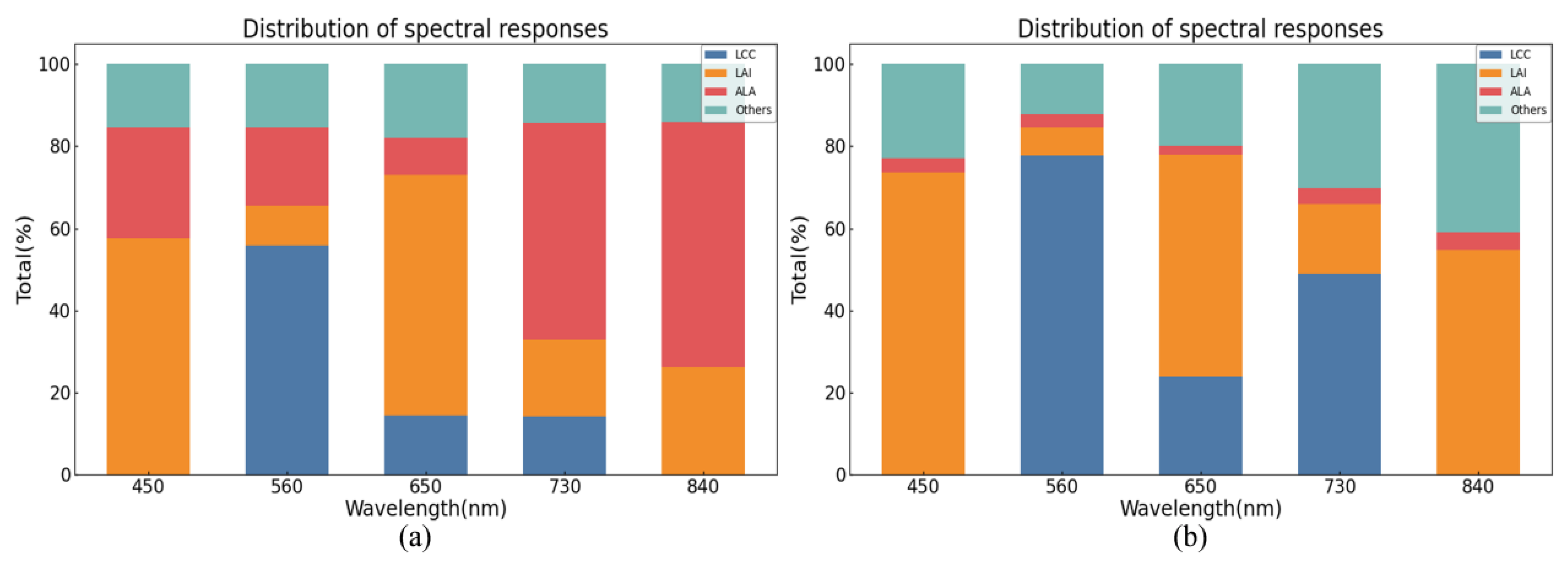
Canopy chlorophyll content (CCC) is an important index for monitoring the growth and estimating the productivity of citrus fruit trees. This study optimized the PROSAIL model by adjusting the average leaf angle (ALA) parameter. A hybrid inversion model was then developed by combining the simulated data with UAV multispectral measurements using machine learning to determine the optimal data fusion ratio for improved citrus CCC prediction. The results show that (1) the most pragmatic accommodation for the hybrid inversion model in this study is the 1:4 ratio of measured data to simulated data; (2) the adjusted ALA (ALAadj) value of citrus fruit trees is 42°, and the spectral response region of the adjusted PROSAIL parameters is more conducive to leaf chlorophyll content (LCC) and the leaf area index (LAI) for CCC modeling; and (3) the ALAadj hybrid inversion model showed significantly better performance than the ALA-unadjusted model under all four machine learning methods, with the peak prediction accuracy, measured by R2, rising from 0.723 to 0.823—a 13.8% increase. The proposed method effectively improves the prediction accuracy of citrus CCCs, demonstrating the strong potential of the ALAadj-based PROSAIL model for UAV-scale CCC monitoring.

1. Introduction

China is a major producer and consumer of citrus fruits, and the citrus industry is the pillar and characteristic industry of many southern provinces [1]. Chlorophyll is an essential factor in citrus growth and plays an indispensable role in photosynthesis [2,3]. Chlorophyll content is commonly used in agricultural productivity studies as a proxy for leaf nitrogen content and an indicator of nitrogen deficiency. Therefore, the rapid and nondestructive acquisition of canopy chlorophyll content (CCC) in citrus trees is crucial for monitoring their growth and health and for enabling precision irrigation. Traditional CCC assays rely on destructive sampling and laboratory analysis, which are time-consuming and labor-intensive, and it is difficult to achieve large-scale dynamic monitoring [4]. In recent years, unmanned aerial vehicle (UAV) multispectral remote sensing has become an important technical means for large-scale CCC inversion of crops because of its high spatiotemporal resolution, high flexibility, and low cost [5,6].
Methods for crop CCC prediction based on UAV multispectral data using empirical models and machine learning [7] usually have problems such as weak generalization ability and lack of stability because of the insufficient number of measured data samples required for model prediction. The radiative transfer model (RTM) has the advantages of clear physical meaning, strong stability and portability, and high prediction accuracy [8]. As a classic tool for RTM, the PROSAIL model can simulate the radiation transport process of vegetation canopies by coupling the leaf-scale PROSPECT model with the canopy-scale SAIL model and is widely used in the inversion of various parameters of plants [9,10,11,12]. However, PROSAIL, as a single-layer homogeneous canopy model, needs to consider the interference of multiple vegetation factors in crop CCC modeling, among which the leaf area index (LAI) and average leaf angle (ALA) are the most important canopy structure parameters that determine the spectral behavior of the canopy. The effects of the LAI and ALA on canopy reflectance are closely related; the LAI controls the degree of attenuation of light within the canopy, and the ALA represents the geometric properties of the canopy, which has a decisive effect on the canopy gap distribution and light interception efficiency [13,14]. Together, they determine canopy anisotropy, making accurate and simultaneous estimation of the LAI and ALA on the basis of canopy spectra difficult [15]. The LAI is measured in the field; thus, introducing prior knowledge of ALA parameters into the PROSAIL model is a way to reduce the uncertainty of crop CCC retrieval [16]. However, it is difficult for the homogeneous canopy assumption of the SAIL model to reflect the three-dimensional heterogeneous structure of real crops, which makes it difficult to improve the spectral simulation and inversion of real crops with prior knowledge of conventional ALA [17]. Since the CCC parameters contain LAI information, the change in the distribution of leaf inclination is the main interference factor in CCC remote sensing inversion [18]. Therefore, the ALA input can be reasonably adjusted for the PROSAIL model to obtain a simulated spectrum that is close to the actual crop spectra. Studies have shown that adjusted ALA (ALAadj) can be obtained by matching the PROSAIL model to the measured spectra and their non-ALA parameters [19]. With respect to the PROSAIL model, ALAadj integrates leaf inclination and canopy heterogeneity information. Adjusting ALA allows PROSAIL simulation to achieve the same canopy gaps as heterogeneous canopies at specific observation angles, thereby altering spectral responses and enhancing the model’s adaptability to specific crops which can improve the adaptability of the model to specific crops [20]. Compared to traditional model parameter inputs, this change represents a more targeted improvement in CCC modeling without including ALA. In previous studies, Sun et al. used machine learning methods to explore the ALAadj values of wheat, soybean, and maize and constructed a simulated dataset to retrieve the LAI and CCC, which achieved good results [21]. However, applications of PROSAIL parameter adjustment remain predominantly focused on annual crops like wheat and maize, an area that is severely understudied for perennial fruit trees such as citrus. To address this gap, this study explores the distribution of the citrus ALA and optimizes the PROSAIL model output based on its simulated spectra and parameter inputs.
Furthermore, while PROSAIL simulation data help expand sample sizes and improve accuracy, they often overlook the role of field measurements and spectral anomalies caused by overidealized defects in simulated datasets [22]. In recent years, researchers have developed a novel hybrid retrieval method that combines PROSAIL with machine learning algorithms to construct a hybrid inversion model [23,24], addressing these limitations. Machine learning algorithms can identify key spectral features through feature importance analysis, reducing the uncertainties caused by parameter coupling [25,26]. By leveraging machine learning, PROSAIL simulation data can be trained to more effectively model complex nonlinear relationships for estimating crop traits [27,28], with enhanced robustness against noise and band gaps—advantages already validated in existing studies. For instance, Sibiya et al. [29] conducted a systematic evaluation of the utility of RTM in remote sensing data retrieval for terrestrial biophysical and biochemical characteristics, demonstrating that integrating PROSAIL with machine learning algorithms creates hybrid models capable of achieving more accurate and reliable vegetation trait estimation.
To address the aforementioned challenges, this study proposes a hybrid modeling approach that integrates UAV multispectral measured data with PROSAIL-simulated spectra using ALA optimization to improve citrus canopy chlorophyll content prediction. The specific research objectives are as follows: (1) combine field small-sample spectral data with PROSAIL-simulated spectra to explore the optimal dataset ratio that preserves measured spectral characteristics; (2) optimize citrus ALA parameters based on UAV-simulated spectra, PROSAIL-simulated spectra, and non-ALA parameters, followed by analysis of spectral responses in optimized PROSAIL models; and (3) compare and analyze the performance of PROSAIL and machine learning hybrid inversion models pre- and post-ALA-adjusted to explore the optimal citrus CCC prediction model.

2. Materials and Methods

2.1. Study Area and Field Test

The experimental area is located at the Guangxi Specialty Crops Research Institute in Qixing District, Guilin city, Guangxi Zhuang Autonomous Region (Figure 1a). The subtropical monsoon climate features mild temperatures, ample sunlight, and abundant rainfall, with long frost-free periods and distinct seasons in which rain and heat coincide. The soil in the experimental area was red soil, the citrus variety was Mercot, the tree was approximately 3 years old, and it was irrigated and fertilized in a unified manner. To ensure methodological reliability, the study introduced Guilin Gongcheng Pengyu Brothers Citrus Demonstration Farm (Figure 1b) as a validation site, which also cultivated 8-year-old Murcott citrus trees. The experimental orchard covers an area of about 50 m × 60 m, and the verification orchard covers an area of about 100 m × 40 m. In each of the experimental and validation areas, 100 sample fruit trees at appropriate intervals were selected (Figure 1).

2.2. UAV Multispectral Data Acquisition

In this study, the DJI Phantom 4 multispectral drone (DJI, Shenzhen, China) was used to capture spectral imagery. The system features six 1-inch, 20-megapixel CMOS sensors, including an RGB sensor for visible light imaging and five monochromatic multispectral imaging sensors. With a maximum takeoff weight of 1487 g and a maximum flight duration of approximately 27 min, the drone delivers comprehensive spectral data, as described in Table 1.
Multispectral imagery was acquired around noon on 10 October 2024, under clear or partially cloudy skies with excellent visibility. The drone was deployed at an altitude of 50 m with 80% heading overlap and 60% side overlap and was mounted vertically downward to achieve a ground sampling distance of approximately 4.16 cm per pixel. A standard calibration plate was placed on the well-lit cement pavement in the experimental area for subsequent radiometric correction and solar variation elimination. In addition, the UAV imagery was first processed in Pix4D to generate a georeferenced mosaic and angle maps. This was followed by a spectral processing chain in ENVI 5.3, consisting of atmospheric (QUAC) and anisotropic (BRDF) corrections, and the extraction of mean reflectance from 30 cm circular ROIs around RTK-located trees. The resulting surface reflectance image is shown in Figure 2. For visual representation, a separate map demonstrating the alignment between the RTK points and the canopy ROIs was generated using ArcGIS 10.6.

2.3. Ground-Measured Data

To determine the ground positions of sample fruit trees and correlate them with UAV multispectral imagery, RTK was used to measure and document the central locations of each tree. Leaves from the upper canopy exposed to sunlight were selected for collection to better represent UAV-scale studies. Ten leaves were evenly sampled from each tree and stored in sealed thermal bags for refrigeration to prevent moisture loss caused by temperature or light exposure. The leaves were subsequently transported to the laboratory, where fresh weight measurements were taken first, followed by soil and plant analysis development (SPAD) measurements using a SPAD-502Plus handheld instrument (Konica Minolta, Tokyo, Japan). Three points were selected for each leaf, and the veins were avoided to measure the SPAD, and the average value of the three points was taken as the blade SPAD value. The final crown SPAD value for the citrus orchard was calculated as the average of 10 leaf SPAD values. With respect to SPAD processing, multiple studies have demonstrated a significant correlation between vegetation SPAD values and absolute leaf chlorophyll content (LCC, unit: μg/cm2) [30,31]. In this study, the inversion model developed by Cerovic et al. [31] (R2 = 0.94) was adopted to convert SPAD values into LCC using the following calculation formula:
L C C = 82.2 × S P A D 135 S P A D
In addition, the LAI-2200C instrument (LI-COR, Lincoln, NE, USA) was used to measure the LAI of sample trees, and the LCC was combined to calculate the citrus CCC. The calculation formula is as follows:
C C C = L A I × L C C
Table 2 shows the main measured parameters and calculated parameter data ranges in this paper.
After this step was completed, the leaf area was measured. Finally, the leaves were dried for 4–5 h at 80 °C. Finally, the dried leaves were weighed, and the dry matter mass of the leaves was recorded for parameter calculation.
C m = W g / S
where C m is the ratio of the dry matter mass of the leaves to the leaf area and W g is the dry matter mass of the leaf and S is the leaf area.
C w = ( W x W g ) / S
where C w is the ratio of the difference between the fresh weight and dry matter mass of the leaf to the leaf area, W x is the fresh weight of the leaves, W g is the dry matter content of the leaves, and S is the leaf area.

2.4. Simulated Spectrum

The PROSAIL-5 model was utilized to simulate canopy spectral characteristics through the coupling of the PROSPECT-5 leaf model and the 4SAIL canopy model [32]. By configuring the multispectral central bands and bandwidths compatible with the UAV systems, five spectral bands were selected from the input parameters in Table 3 to obtain the crop canopy spectra, which were subsequently used to train a crop CCC prediction model.
At the leaf level, the Cab value was set between 32 and 100 μg/cm2 on the basis of the measured data. Carotene accounts for 25% of the Cab value content and varies with it [18]. The leaf structure parameter (N) significantly affects the spectral characteristics; therefore, its range was defined as 1.0–2.0 with a narrow step size. Since water absorption bands are typically not used for vegetation chlorophyll retrieval and their measured values show minor fluctuations, both dry matter content (Cm) and equivalent water thickness (Cw) were fixed at the average measured values.
With respect to canopy structure, the LAI, which has a significant spectral contribution, is strictly controlled within the measured ranges. The initial (ALA) value calculated from the LIDFa (in degrees) can be expressed as ALA = 45–360 × LIDFa/π2 [33], ranging from 10° to 80°. To determine the soil structural coefficients, an ASD FieldSpec Pro 4 spectrometer (ASD Inc., Boulder, CO, USA) was used in this study to collect spectral data of bare soil exposed to sunlight and shadow beneath the tree canopy, covering wavelengths from 0.1 to 0.4. Utilizing drone orthoimage data, the observation zenith angle was set to 0°, while the solar zenith angle was fixed at 30°.

2.5. Research Methods

To achieve high-precision prediction of multispectral small-sample citrus CCCs using drones, this study optimized the PROSAIL model with ALAadj values. By integrating simulated data from ALA optimization and UAV multispectral measurement data, we constructed a hybrid inversion model for citrus CCCs through machine learning methods. The RMSE and R2 metrics were used to evaluate and determine the optimal inversion model for determining the citrus CCC.

2.5.1. Optimization and Adjustment of ALAs

The heterogeneous canopy structure of crops does not align with the assumption of a homogeneous canopy. In the PROSAIL model, inputting parameters based on conventional prior knowledge fails to adequately represent actual crop traits through spectral characteristics. The leaf-scale factor has no influence on canopy heterogeneity in the PROSPECT model. Within the SAIL model, the spectral sensitivity of the LAI and ALA [34] remains paramount. In the PROSAIL model for CCC inversion modeling, the CCC contains LAI and LCC information, and the sensitive response areas of the LAI and ALA overlap. Therefore, in the SAIL model, the simulated spectrum closer to the actual crop spectrum can be obtained by adjusting the ALA, which is more conducive to CCC modeling research. Additionally, considering the critical contribution of ALAs to multispectral bands, adjusting the ALA in crop CCC inversion modeling, which incorporates LAI information, is highly important for reducing the spectral response.
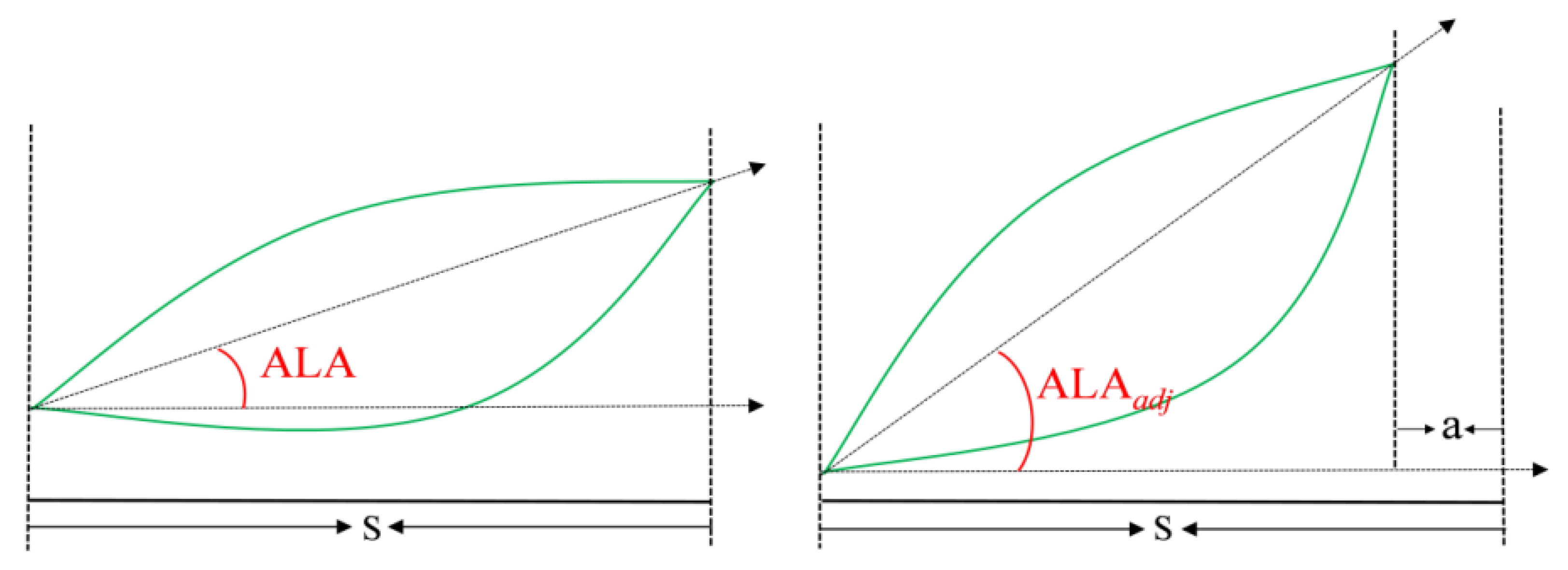
The ALA is determined by the leaf angle distribution (LAD) function, denoted as LIDFa and LIDFb. Since LIDFb has a minimal effect on canopy reflectance [35], the ALA is primarily determined by LIDFa. The magnitude of the ALA is predominantly determined by crop type, with each crop exhibiting distinct growth patterns that make the ALA less susceptible to external factors. In the PROSAIL model, optimizing the ALA requires not only spectral data but also measured LAI measurements. Additionally, measured LCC are incorporated into both PROSAIL simulations and CCC modeling as supplementary data. The role of ALA optimization is illustrated in Figure 3. Two identical-sized leaves can achieve different canopy gaps under the same ground area by adjusting their ALA distribution, thereby altering the light reflection efficiency. Here, S represents the ground area, and a denotes the canopy gap.
The multispectral data used in this study consist of only five spectral bands, which occupy minimal memory. Given that the random forest algorithm is recognized for its accurate predictions and robust error tolerance, making it particularly suitable for large-scale dataset processing [36], we employed random forest regression to evaluate the impact of the ALA and other vegetation parameters on reflectance. On the basis of the measured spectral data and non-ALA parameter adjustments, we refined the ALA configuration of the PROSAIL model. The study generated 10,000 simulated datasets for model training, with the ALA parameter bounded between 10° and 80°. The hyperparameter optimization for the RFR was conducted through a grid search over the specified parameters (n_estimators: [100, 200], max_depth: [10, 20, None], min_samples_split: [2, 5], min_samples_leaf: [1, 2]), which involved a total of 120 distinct model trainings. The adjusted ALA value for citrus (denoted as ALAadj) is expressed as follows:
A L A a d j = R F R   ( S P E C , L A I , L C C )
where SPEC, LAI, and LCC represent the measured spectral reflectance, sample tree LAI, and LCC measurements, respectively. The PROSAIL model can be updated by inputting adjusted ALA values to generate simulated spectra tailored for specific crops.

2.5.2. Hybrid Modeling and Precision Evaluation

The inversion of the PROSAIL model typically employs two approaches to obtain fitting parameters that match measured data: lookup tables and machine learning methods [37]. While lookup tables utilize a pixel-by-pixel iterative search mechanism and discrete parameter sampling, they struggle to adequately capture the continuous nonlinear relationship between vegetation parameters and spectral responses. This results in low computational efficiency and susceptibility to local optima because of the presence of loss functions [38]. In contrast, machine learning learns complex nonlinear mappings from RTM-simulated data during training, enabling rapid parameter inversion in prediction stages while effectively decoupling sensitivity conflicts between parameters [39]. To investigate differences in citrus CCC prediction accuracy between hybrid inversion models using UAV multispectral imagery and PROSAIL-simulated spectra with adjusted ALAs, this study employed four machine learning methods: partial least squares regression (PLSR), Gaussian process regression (GPR), random forest regression (RFR), and support vector regression (SVR).
PLSR is a multivariate regression method designed for modeling high-dimensional collinear data. By extracting latent variables (principal components) from independent and dependent variables, it achieves both dimensionality reduction and feature selection while demonstrating efficient performance even with small sample sizes [40]. GPR is a nonparametric model based on Bayesian frameworks that employs Gaussian processes to describe data distributions and covariance functions to characterize relationships between samples [41]. Its strength lies in providing uncertainty intervals for prediction outcomes, making it suitable for small-to-medium sample sizes and nonlinear problems [42]. RFR, an ensemble learning method, involves prediction through voting or averaging multiple decision trees [43], resulting in features such as overfitting resistance, high-dimensional feature adaptability, support for nonlinear relationships, and feature importance evaluation. It has significant advantages in large-scale data processing [44]. SVR, a machine learning approach rooted in statistical theory [45], maps data into high-dimensional space using kernel functions for linear regression while minimizing structural risk through sensitivity loss functions. Its strengths include handling small sample sizes, addressing nonlinear challenges, and exhibiting robustness against outliers [46].
This study utilized four machine learning algorithms to conduct preliminary hybrid predictions using both measured and simulated data, calculating the mixing ratio between the two data types according to Equation [47]:
S = n × I
where S is the simulated data volume, n is the sample size, and I is an integer. I starts from 0 and gradually increases. While the simulated data are fully used to expand the sample size and improve the accuracy, the optimal value is determined when the measured data characteristics are not lost, the model is stable and no overfitting occurs.
In this paper, the coefficient of determination R2 and root mean square error (RMSE) were used to evaluate the fitting performance of the model. To evaluate the uncertainty associated with model performance estimates, 95% confidence intervals for R2 and RMSE were computed using the bootstrap resampling method with 1000 replicates. The calculation formula is as follows, where R2 is closer to 1, indicating that the model fitting effect is better, and the RMSE is closer to 0, indicating that the prediction value and measured value have smaller errors.
R 2 = i = 1 n y i ~ y ¯ 2 i = 1 n y i y ¯ 2
R M S E = i = 1 n ( y ~ y i ) 2 / n
where n is the number of samples; i = 1, 2, 3, …, n ; y i ~ and y i represent the predicted value and measured value of the citrus CCC, respectively; and y ¯ is the average value of the measured value of the citrus CCC.

3. Results and Analysis

3.1. PROSAIL Parameter Sensitivity Analysis

Sensitivity analysis (SA) aims to quantify the impact of individual input variables on model outcomes, helping identify the contributions of input parameters to output variables. To evaluate the potential of UAV multispectral technology in citrus biochemical variable analysis, conducting SA on spectral bands within its detection domain through the PROSAIL model is a prerequisite. In this study, using MATLAB R2018a and ARTMO tools, we first performed local sensitivity analysis (LSA) to identify parameters with minimal influence on the model results—Cab, N, LAI, ALA, and Psoil—which were fixed values without further analysis. A global sensitivity analysis (GSA) was subsequently conducted on these five parameters, and the results are shown in Figure 4.
According to the parameter range inputs in Table 2, among the five multispectral bands of the drones, the spectra at 450 nm and 650 nm are most significantly affected by the LAI (Figure 4). At approximately 450 nm, chlorophyll and carotenoids have strong absorption bands, which are blue light bands. Blue light is easily intercepted by upper leaves, and the reflectivity depends mainly on the leaf density [48]. At 650 nm, the red light band is the main absorption peak of chlorophyll, and the absorption is close to saturation. The reflectivity depends mainly on the number of leaf layers, after which the contribution of chlorophyll gradually decreases. The reflectance in both the blue and red light bands is primarily determined by the depth of light penetration within the canopy, whereas the LAI directly affects the leaf layer count, thus exerting the most significant influence. At 560 nm, which is located in the chlorophyll absorption valley (green light reflection peak), the reflectance becomes highly sensitive to changes in Cab. Owing to the strong penetration capability of green light, the impact of increased LAI on reflectance is less pronounced than that in the blue and red bands [49]. The spectral bands at 730 nm and 840 nm are subsequently predominantly influenced by ALA. This outcome arises from two factors: first, the ALA lacks measured values and has a broad parameter range; second, the red edge region near 730 nm is significantly affected by leaf internal structures (e.g., spongy tissue), where the ALA indirectly regulates the red edge slope through altered light scattering paths. Higher ALA levels lead to multiple light scatterings within the canopy, thereby enhancing red edge reflectance. At 840 nm, the near-infrared region has little absorption of leaves, and the reflectivity is determined mainly by the crown structure. The measured range of the LAI in the sample trees in this paper is small; thus, the reflectivity near the near-infrared band is most affected by the ALA.
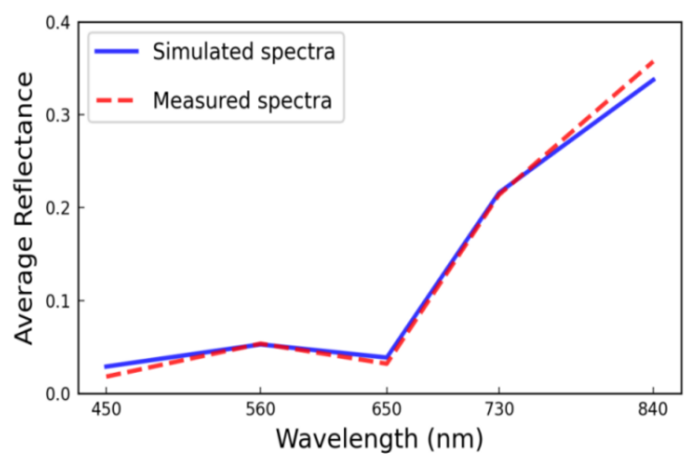
According to the sensitivity analysis and input parameters, the simulated spectrum was obtained, and the average values of 10,000 simulated spectra and 100 measured spectral reflectances were calculated. The results are shown in Figure 5.
As shown in Figure 5, the simulated spectrum and the measured spectrum have a good fitting effect. The correlation between them reaches 99%; therefore, the simulation spectrum can represent the measured spectrum well as an expanded sample.

3.2. Experimental Analysis of the Mixing Ratio Between Measured and Simulated Data

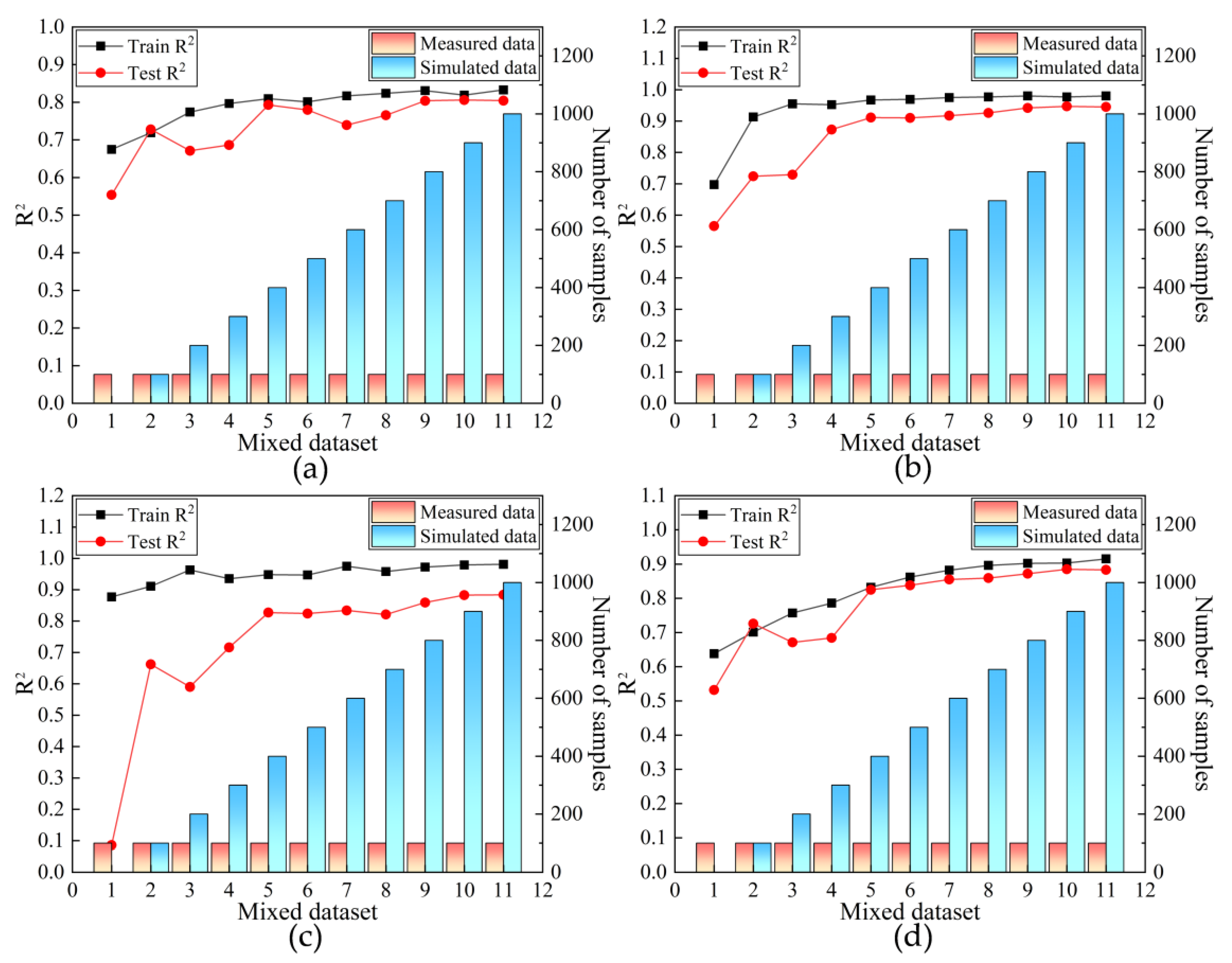
To establish a high-precision inversion model while preserving the characteristics of the measured data to the greatest extent, it is necessary to meet the condition of achieving high accuracy and stable model performance with as little simulated data as possible. This study employed four machine learning algorithms, adopted a 5-fold cross-validation scheme, and provided the detailed hyperparameter grids used for grid search with the four algorithms (Table 4). The proportion of simulated data in the hybrid inversion model and its corresponding model performance were calculated using Equation (6), with the results shown in Figure 6.
Figure 6 shows a horizontal axis ranging from Scale 1 to Scale 11, which represents different data sample sizes. Scale 1 corresponds to the original measured data without simulated data (I = 0, Formula 6), comprising 100 samples. Scale 2 represents the scenario with I = 1, where the measured data-to-simulated data ratio is 1:1 (200 samples), and so forth. In this study, the test set and training set are divided at a 1:4 ratio. The R2 values in the training set remain relatively stable, showing steady improvement as the sample data increase, whereas the R2 values of the test set fluctuate significantly. As shown in Figure 6a, adding simulated data to the training set substantially improved accuracy over the original dataset, with R2 rising from 0.554 at Scale 1 to 0.728 at Scale 2. Despite this gain, Scale 2 would only be the optimal choice if model stability were not a concern, as it requires the least simulated data and allows for the greatest reliance on the features of the measured data. However, Scales 3–4 demonstrate poor accuracy, indicating that insufficient simulated data compromise model stability. At Scale 5 (I = 4), the test set R2 values achieve significant improvement again. Although subsequent scales show continued fluctuations, they remain relatively stable compared with the first four scales, with R2 values consistently above 0.7. The highest R2 value occurs at Scale 9, but this proportionally increases the simulated data, causing severe feature loss in the measured data. Since training data weights were not allocated in this part of the experiment, the accuracy levels primarily stem from the simulated data. Consequently, the absolute accuracy values are not the criterion for evaluating model performance; the key lies in the trend of accuracy change. As evidenced by the performance in Figure 6b–d, all show results similar to those in Figure 6a, namely a significant accuracy improvement at Scale 5, after which the model stabilizes. Taking all factors into consideration, we conclude that Scale 5 is the optimal scale, corresponding to an I value of 4. This indicates that a measured-to-simulated data ratio of 1:4 represents the most pragmatic accommodation for this experimental framework.

3.3. Comparative Analysis of the ALA Optimization Results

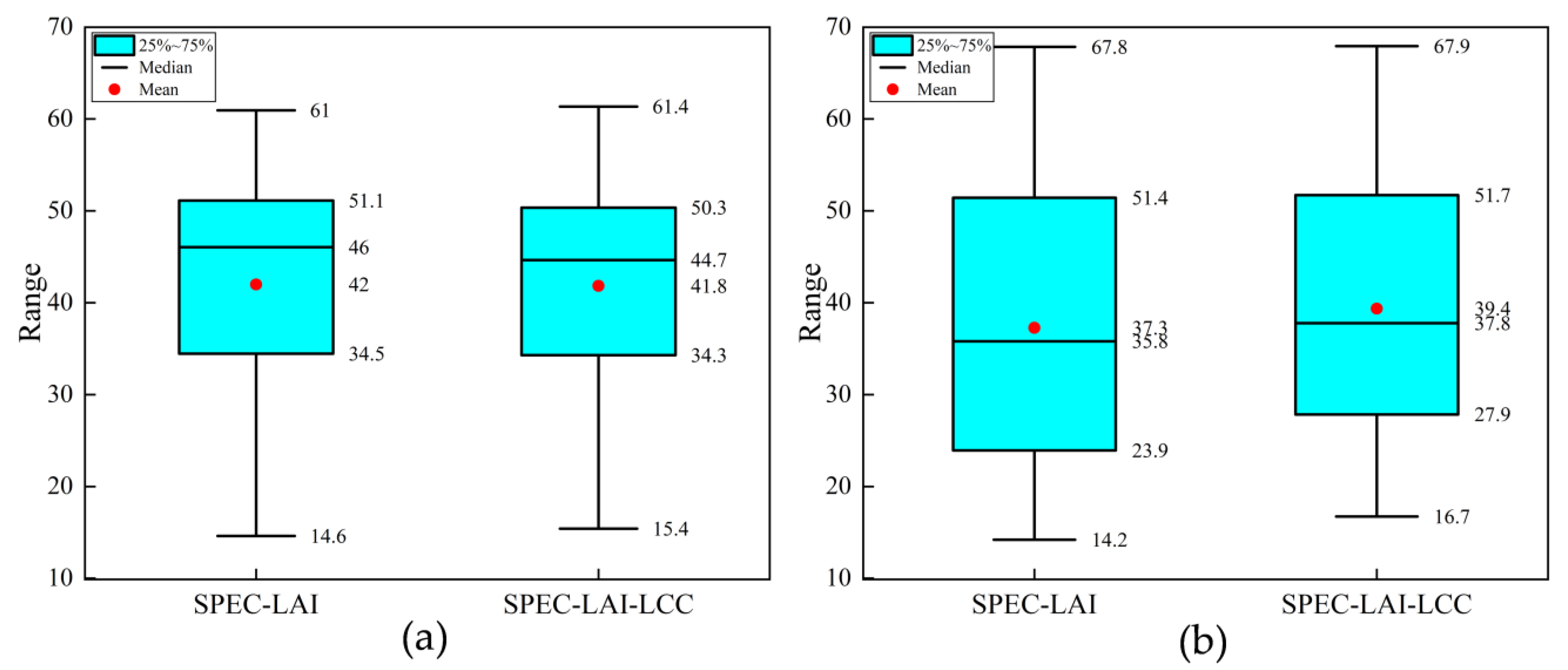
Since the assumption of the leaf angle distribution in the PROSAIL model differs from that in actual field conditions, we developed an RFR-based ALA optimization model (Section 2.5.1) using simulated spectral data and measured LAI and LCC. To validate the rationality of the optimization adjustments, validation zones with varying growth environments and tree ages were introduced for comparative verification of the citrus ALA. To investigate the role of the measured LAI and LCC in the ALA optimization model, this study employed two distinct training datasets: the first combining simulated spectral data with the measured LAI and the second containing measured LCC data. Both datasets were utilized in PROSAIL optimization, yielding highly consistent citrus ALAadj values (Figure 7).
As shown in Figure 7, the ALA distribution in the experimental area for citrus ranged from 14° to 61°, with a peak concentration between 34° and 51°. Compared with Dataset 1, the box plot for Dataset 2 demonstrates more concentrated quantiles and closer proximity between the median and mean values, indicating that adding LCC would be more advantageous for the study. However, the overall optimized results for the ALAs remained stable regardless of whether LCC was included. In contrast, the validation area showed a more dispersed distribution, with slightly lower median and mean values. This may be attributed to the older tree age and more abundant foliage, which resulted in slower growth patterns with greater but gentler leaf inclination angle variations. Overall, the similarity in the ALA levels between the two sample areas validates the results. Therefore, 42° was adopted as the adjusted value for citrus ALA in this study.
Since the multispectral responses of the PROSAIL model primarily consist of LCC, LAI, and ALA, the parameters are categorized into four types: LCC, LAI, ALA, and others. The unadjusted spectral response of the ALA parameters is shown in Figure 8a. ALA exhibits significant responses across all the bands, particularly at 730 nm and 840 nm, where it even temporarily exceeds the combined values of LCC plus LAI plus others. This phenomenon is detrimental to CCC prediction, which incorporates LCC and LAI information. After adjusting for the ALA, the spectral responses of the LCC and LAI markedly increase, which undoubtedly strengthens the correlation between the spectral data and the CCC prediction, thereby improving the citrus CCC forecasting accuracy (Figure 8b).

3.4. Performance Evaluation of the ALAadj Hybrid Inversion Model

This study employed four machine learning algorithms to construct a hybrid inversion model. The dataset was partitioned using a reproducible stratified sampling method, initialized with a fixed random seed (42). The training set consisted of 350 simulated data samples and 50 measured data samples, totaling 400 training samples. The testing set contained the remaining 50 simulated data samples and 50 measured data samples. To address the data source imbalance, a weighting scheme was applied where both simulated and measured data each account for 50% of the total training weight, ensuring the prominence of measured data features during model optimization. Table 5 presents the dataset sampling scheme.
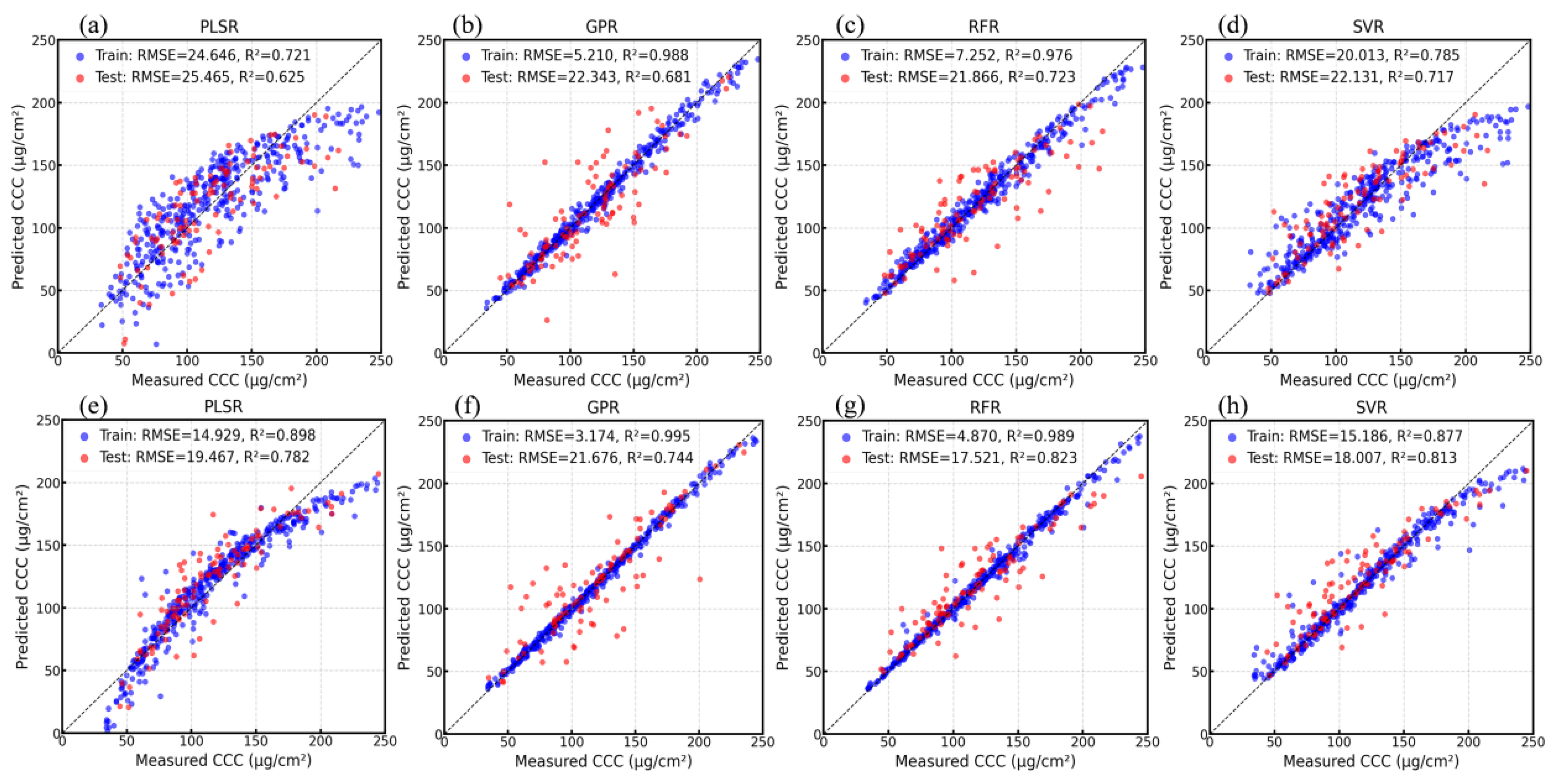
A comparison of citrus CCC prediction accuracy among the four machine learning algorithms using this hybrid model is shown in Figure 9, with two precision evaluation results (adjusted and unadjusted for ALA) displayed separately. The ALAadj hybrid model’s CCC prediction results after ALA adjustment through the PROSAIL model are shown in Figure 9e–h. The data reveal that under identical sample sizes, all four machine learning algorithms demonstrated more concentrated predictions in both the training and test sets, with their performance significantly outperforming that of the ALA-unadjusted hybrid model (Figure 9a–d). Among the models optimized with ALA adjustments, the PLSR algorithm demonstrated the most significant performance improvement, achieving an R2 value increase of 0.157 and a reduction of 5.998 μg/cm2 in the RMSE. This improvement occurred because the PLSR algorithm performed poorly in the ALA-unadjusted hybrid model, showing scattered prediction distributions across the training and test sets with greater potential for improvement. Notably, it was underestimated when high-value citrus CCCs were predicted. The GPR algorithm showed minimal gains and failed to replicate its high precision in test data, performing worst in both robustness and accuracy. The SVR algorithm delivered balanced results: maintaining high precision while achieving substantial accuracy gains and demonstrating the best robustness against overfitting. However, it slightly overestimated the low-value citrus CCC and underestimated the high-value cases. The RFR algorithm achieved the most notable performance improvement, with R2 values increasing from 0.723 to 0.823 and the RMSE decreasing by 4.345 μg/cm2. The ALA-unadjusted hybrid model had the best performance compared to other methods. After adjusting the ALA, it still greatly improved, and there was no overestimation or underestimation.

3.5. Performance Comparison Analysis of the ALAadj Hybrid Inversion Model in the Validation Area

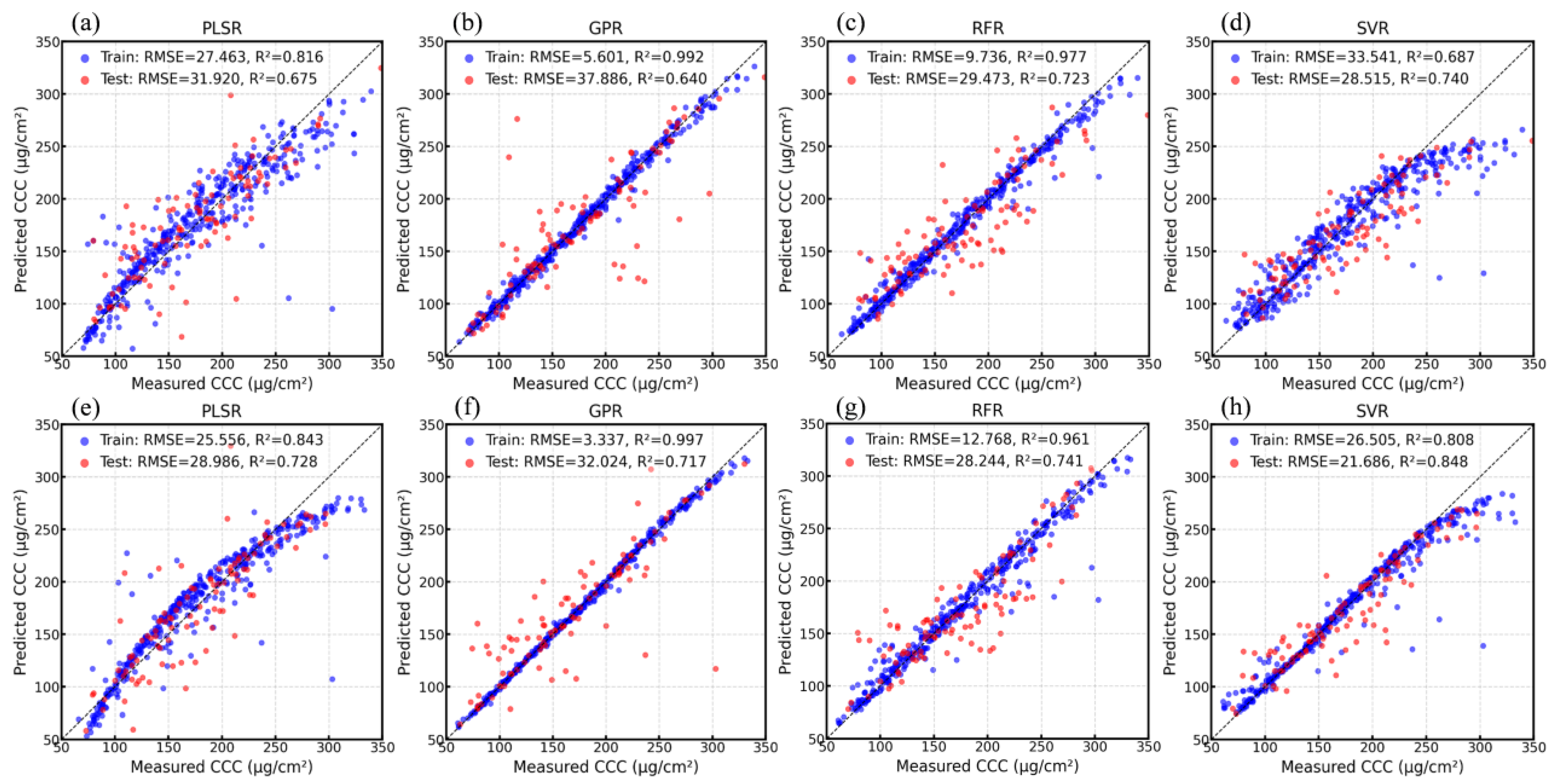
In this study, identical experimental treatments were conducted in the validation zone, as described in Section 3.4, and the results were comparable to those of the experimental zone models (Figure 10a–h). Compared with its unadjusted counterpart, the ALA-adjusted hybrid model demonstrated improved accuracy, further validating the rationality of our optimized ALA adjustment for citrus applications and confirming that the proposed method significantly enhances prediction precision. Notably, the performance of PLSR, GPR, and SVR closely aligned with that of the experimental zone data, whereas the accuracy of RFR improved slightly, which was not as obvious as the improvement in the performance of the experimental area data. This finding indicates that the influence of algorithm selection on model precision may not surpass that of data quality. In contrast, SVR maintained its signature strengths in terms of high accuracy and robustness against overfitting.
Table 6 summarizes the performance comparison of the experimental area and the verification area for the four machine learning methods for predicting citrus CCC under the hybrid inversion model with or without ALA adjustment.

4. Discussion

In this study, a machine learning hybrid modeling inversion method that combines PROSAIL-simulated spectral data optimized through the ALA with UAV-measured multispectral observations is proposed to enhance citrus CCC prediction performance. Using RFR for spectral parameter analysis of PROSAIL simulations, we achieved the first successful optimization of ALA parameters in citrus trees. By integrating the measured spectra with non-ALA parameters, we calculated ALA values consistent with real-world heterogeneous canopy conditions, which were successfully applied to citrus CCC prediction.
As a structural parameter in PROSAIL models, the ALA characterizes the random spatial distribution of leaves. The configuration of the ALA determines spectral transmission within vegetation, thereby influencing its effective reception range [50]. In the RFR-based ALA optimization scheme, spectral data serve as the primary influencing factor. Additionally, the LAI provides essential measured data for parameterization adjustments. The results of this study demonstrate that when the measured LAI and canopy spectral data are used, ALAadj is stable, regardless of whether LCC is involved (Figure 7). Of course, incorporating LCC enhances result stability. Through optimization of the citrus ALA, the spectral response of the PROSAIL parameters becomes more aligned with both LCC and LAI. This alignment is particularly evident for the LAI, as the LAI and ALA exhibit overlapping spectral response regions that are challenging to distinguish through spectral retrieval [51]. Reducing the spectral response of the ALA in sensitive bands effectively amplifies the spectral influence of the LAI. Similar effects occur in LCC high-sensitivity green and red-edge bands, which are beneficial for improving CCC modeling. In this study, the optimization of the citrus ALA not only significantly improved the computational efficiency of the PROSAIL model, making the simulated spectra more consistent with actual crop spectra but also substantially enhanced the model prediction accuracy, providing crucial insights for practical applications of the PROSAIL model. Notably, since the optimized ALA parameters were derived from simulated spectra (which correspond to ALA measurements) and measured spectra with their respective parameters—two distinct datasets—theoretically, the 42° value might not represent the most accurate ALA measurement for citrus. To address this, we conducted validation and comparison using a validation zone, ensuring the reliability of the results.
The PROSAIL model simplifies scenarios and parameters, providing high-precision simulation data with large sample sizes while exhibiting overidealization flaws. However, measured spectra are susceptible to environmental, equipment, and growth stage influences, making it challenging to align simulated spectra with actual measurements. This limitation restricts vegetation parameter hybrid inversion based on the PROSAIL model. Therefore, under fixed measurement data samples, this study conducted experimental comparisons of simulation data from limited to extensive sample sizes, aiming to obtain a model with high performance accuracy and stability at smaller sample scales to address overidealization issues. Additionally, with respect to the PROSAIL parameter sensitivity analysis results, for multispectral data with only five bands, some less sensitive parameters can be omitted from the input ranges. The measured spectra may be influenced by multiple external factors beyond those affected by PROSAIL parameters. Different versions of the PROSAIL model have varying parameters, and the measured parameters are subject to various errors. Thus, strictly adhering to measured ranges for low-sensitivity parameters may not yield the expected outcomes. As shown in Section 3.1, discrepancies between the simulated and measured spectra remain inevitable. For chlorophyll assessment, SPAD provides a practical and efficient method for field data collection. However, as the PROSAIL model requires absolute leaf chlorophyll content as an input, a conversion from SPAD values to LCC was necessary. The observed transformation, where SPAD values (38–74) were converted to LCC values (32–99 μg/cm2), resulted in a slight contraction at the lower end and a more pronounced expansion at the higher end of the range. This pattern is consistent with the slightly concave nonlinear relationship between SPAD readings and actual chlorophyll content, as reported by Cerovic et al. [31], and reflects the natural variability inherent in such physiological measurements.
In constructing the hybrid inversion model, this study addresses the significant impact of simulated versus measured data on prediction outcomes. To optimize performance, we innovatively implemented a controlled weighting method for training dataset allocation. This dual approach preserves measured data characteristics while maximizing the advantages of the simulated data. All four machine learning algorithms employed this data distribution strategy, ensuring that the discrepancies in prediction accuracy originate from algorithmic design rather than data sources. The results demonstrate no inherent superiority among these algorithms, with only applicable variations observed. For instance, while the GPR outperforms all the other models on the training datasets, its failure to replicate the performance on the test sets indicates its unsuitability for hybrid models with sampling biases. Given inherent model differences, absolute fairness in parameter allocation cannot be guaranteed. When precision variations remain minimal, relative fairness in evaluating model applicability becomes the appropriate approach [52]. Furthermore, this study employs 500 data samples for experimentation, making the model’s adaptability to sample size crucial for performance. For instance, PLSR proves optimal for spectral prediction in small sample scenarios. While GPR delivers the best performance in medium–small sample ranges, its heavy reliance on kernel functions leads to oscillatory results. SVR shows diminishing advantages with increasing sample sizes and rising computational costs but remains a viable choice in small-to-medium sample scenarios. When massive datasets are being handled, RFR emerges as the preferred method because of its incremental learning capability, which accommodates ultra-large datasets, whereas other approaches face computational bottlenecks. Given the inevitable trend of large-scale agricultural cultivation in future agriculture, RFR algorithms with large-sample hybrid models demonstrate promising prospects for predictive modeling.
In addition, this study was conducted exclusively at the UAV multispectral scale. Future research could undertake synchronous testing and comparisons at UAV hyperspectral and even satellite scales. It could also involve monitoring citrus canopies across different growth stages and environments, and exploring the model’s performance when transferred to various phenological stages to further validate the generalizability of the proposed method.

5. Conclusions

In this study, the distribution of ALAs in citrus fruit trees was investigated through parameter adjustments in the PROSAIL model to address homogenized canopy issues. The PROSAIL model was optimized by using the ALAadj value to change the spectral response of the model parameters. The simulated data of the ALA optimization and the multispectral measured data of the UAV were combined, and the machine learning method was used to find the optimal data mixing ratio to solve the defect of overidealization of the simulated data, and a hybrid inversion model was constructed to improve the prediction of citrus CCCs. Key findings include the following:
(1)
A 1:4 ratio of measured to simulated data was identified as the most pragmatic accommodation for the hybrid inversion model in this study;
(2)
The ALAadj value in the study area was 42°, with adjusted PROSAIL parameters showing enhanced spectral response regions favorable for LCC and LAI modeling in the CCC;
(3)
Compared with the unadjusted versions, the ALAadj hybrid inversion model demonstrated significant performance improvements across the four machine learning methods, with the peak R2 increasing by 13.8% from 0.723 to 0.823 and the RMSE decreasing by 19.9% from 21.866 μg/cm2 to 17.521 μg/cm2.

Author Contributions

Conceptualization, Y.H. and M.L. and S.D.; methodology, S.D.; software, S.Y. and R.W.; validation, Z.M., Y.S. and J.Y.; formal analysis, Y.H.; investigation, Y.H. and M.L.; resources, R.W.; data curation, Z.M. and J.Y.; writing—original draft preparation, Y.H.; writing—review and editing, Y.H. and S.D.; visualization, S.D. and S.Y.; supervision, S.D.; project administration, R.W.; funding acquisition, S.D. All authors have read and agreed to the published version of the manuscript.

Funding

This study was supported by the Key Research and Development Program Project of Guangxi (No. 2025FNFN97094); the Natural Science Foundation of Guangxi (No. 2023JJA150097); the Guilin City Science Research and Technology Development Plan Project (No. 20230120-13).

Data Availability Statement

All data generated or analyzed during this study are included in this article.

Conflicts of Interest

Author Rongbin Wang was employed by the company Shandong Mingjia Survey and Surveying Co., Ltd. The remaining authors declare that the research was conducted in the absence of any commercial or financial relationships that could be construed as a potential conflict of interest.

References

  1. Zhou, M.W.; Fu, C.N.; Wang, C.C.; Xu, Y.J.; Jiang, M.L.; Xiao, Y.H.; Lu, F. Analysis of Countermeasures for the High-quality Development of Guilin’s Citrus Industry. South. Hortic. 2025, 36, 62–69. [Google Scholar]
  2. Wang, Y.N.; Sun, Y.; Chen, Y.N.; Wu, C.Y.; Huang, C.P.; Li, C.; Tang, X.G. Non-linear correlations exist between solar-induced chlorophyll fluorescence and canopy photosynthesis in a subtropical evergreen forest in Southwest China. Ecol. Indic. 2023, 157, 111311. [Google Scholar] [CrossRef]
  3. Lawson, T.; Chabrand, S.V. Imaging Spatial and Temporal Variation in Photosynthesis Using Chlorophyll Fluorescence. In Photosynthesis: Methods and Protocols; Methods in Molecular Biology; Springer: New York, NY, USA, 2024; Volume 2790, pp. 293–316. [Google Scholar] [CrossRef]
  4. Xu, Z.H.; He, A.Q.; Zhang, Y.W.; Hao, Z.B.; Li, Y.F.; Xiang, S.Y.; Li, B.; Chen, L.Y.; Yu, H.; Shen, W.L.; et al. Retrieving chlorophyll content and equivalent water thickness of Moso bamboo (Phyllostachys pubescens) forests under Pantana phyllostachysae Chao-induced stress from Sentinel-2A/B images in a multiple LUTs-based PROSAIL framework. For. Ecosyst. 2023, 10, 100108. [Google Scholar] [CrossRef]
  5. Cheng, J.P.; Yang, H.; Qi, J.B.; Sun, Z.D.; Han, S.Y.; Feng, H.K.; Jiang, J.Y.; Xu, W.M.; Li, Z.H.; Yang, G.J.; et al. Estimating canopy-scale chlorophyll content in apple orchards using a 3D radiative transfer model and UAV multispectral imagery. Comput. Electron. Agric. 2022, 202, 107401. [Google Scholar] [CrossRef]
  6. Cheng, Q.; Xu, H.; Fei, S.; Li, Z.; Chen, Z. Estimation of Maize LAI Using Ensemble Learning and UAV Multispectral Imagery under Different Water and Fertilizer Treatments. Agriculture 2022, 12, 1267. [Google Scholar] [CrossRef]
  7. Wang, J.; Zhang, Y.; Han, F.; Shi, Z.; Zhao, F.; Zhang, F.; Pan, W.; Zhang, Z.; Cui, Q. Estimation of Canopy Chlorophyll Content of Apple Trees Based on UAV Multispectral Remote Sensing Images. Agriculture 2025, 15, 1308. [Google Scholar] [CrossRef]
  8. Feng, H.; Fan, Y.; Yue, J.; Ma, Y.; Liu, Y.; Chen, R.; Fu, Y.; Jin, X.; Bian, M.; Fan, J.; et al. Enhancing potato leaf protein content, carbon-based constituents, and leaf area index monitoring using radiative transfer model and deep learning. Eur. J. Agron. 2025, 166, 127580. [Google Scholar] [CrossRef]
  9. Verhoef, W. Light scattering by leaf layers with application to canopy reflectance modeling: The SAIL model. Remote Sens. Environ. 1984, 16, 125–141. [Google Scholar] [CrossRef]
  10. Zhang, C.J.; Chen, Z.B.; Yang, G.J.; Xu, B.; Feng, H.K.; Chen, R.Q.; Qi, N.; Zhang, W.J.; Zhao, D.; Cheng, J.P.; et al. Removal of canopy shadows improved retrieval accuracy of individual apple tree crowns LAI and chlorophyll content using UAV multispectral imagery and PROSAIL model. Comput. Electron. Agric. 2024, 221, 108959. [Google Scholar] [CrossRef]
  11. Sun, B.; Wang, C.; Yang, C.; Xu, B.; Zhou, G.; Li, X.; Xie, J.; Xu, S.; Liu, B.; Xie, T.; et al. Retrieval of rapeseed leaf area index using the PROSAIL model with canopy coverage derived from UAV images as a correction parameter. Int. J. Appl. Earth Obs. Geoinf. 2021, 102, 102373. [Google Scholar] [CrossRef]
  12. Yang, N.; Zhang, Z.; Yang, X.; Zhang, J.; Zhang, B.; Xie, P.; Wang, Y.; Chen, J.; Shi, L. UAV-based stomatal conductance estimation under water stress using the PROSAIL model coupled with meteorological factors. Int. J. Appl. Earth Obs. Geoinf. 2025, 137, 104425. [Google Scholar] [CrossRef]
  13. Wang, R.; Sun, Z.; Bai, W.; Wang, E.; Wang, Q.; Zhang, D.; Zhang, Y.; Yang, N.; Liu, Y.; Nie, J.; et al. Canopy heterogeneity with border-row proportion affects light interception and use efficiency in maize/peanut strip intercropping. Field Crops Res. 2021, 271, 108239. [Google Scholar] [CrossRef]
  14. Li, K.; Jiang, C.; Guan, K.; Wu, G.; Ma, Z.; Li, Z. Evaluation of average leaf inclination angle quantified by indirect optical instruments in crop fields. Int. J. Appl. Earth Obs. Geoinf. 2024, 134, 104206. [Google Scholar] [CrossRef]
  15. Casa, R.; Baret, F.; Buis, S.; Lopez-Lozano, R.; Pascucci, S.; Palombo, A.; Jones, H.G. Estimation of maize canopy properties from remote sensing by inversion of 1-D and 4-D models. Precis. Agric. 2010, 11, 319–334. [Google Scholar] [CrossRef]
  16. Jacquemoud, S.; Verhoef, W.; Baret, F.; Bacour, C.; Zarco-Tejada, P.J.; Asner, G.P.; Francois, C.; Ustin, S.L. PROSPECT plus SAIL models: A review of use for vegetation characterization. Remote Sens. Environ. Interdiscip. J. 2009, 113, S56–S66. [Google Scholar] [CrossRef]
  17. Pan, Y.; Wu, W.; He, J.; Zhu, J.; Su, X.; Li, W.; Li, D.; Yao, X.; Cheng, T.; Zhu, Y.; et al. A novel approach for estimating fractional cover of crops by correcting angular effect using radiative transfer models and UAV multi-angular spectral data. Comput. Electron. Agric. 2024, 222, 109030. [Google Scholar] [CrossRef]
  18. Jiao, Q.; Sun, Q.; Zhang, B.; Huang, W.; Ye, H.; Zhang, Z.; Zhang, X.; Qian, B. A Random Forest Algorithm for Retrieving Canopy Chlorophyll Content of Wheat and Soybean Trained with PROSAIL Simulations Using Adjusted Average Leaf Angle. Remote Sens. 2021, 14, 98. [Google Scholar] [CrossRef]
  19. Danner, M.; Berger, K.; Wocher, M.; Mauser, M.; Hank, T. Fitted PROSAIL Parameterization of Leaf Inclinations, Water Content and Brown Pigment Content for Winter Wheat and Maize Canopies. Remote Sens. 2019, 11, 1150. [Google Scholar] [CrossRef]
  20. Yang, G.; Qin, J.; Wang, L.; Fang, S.; Li, W.; Chen, Y.; Gong, Y.; Dian, Y.; Sun, C.; Wang, J.; et al. Accurate solution of the SAIL model by leaf inclination angle calculation based on laser point clouds. Geo-Spat. Inf. Sci. 2025, 28, 722–740. [Google Scholar] [CrossRef]
  21. Sun, Q.; Jiao, Q.; Chen, X.; Xing, H.; Huang, W.; Zhang, B. Machine Learning Algorithms for the Retrieval of Canopy Chlorophyll Content and Leaf Area Index of Crops Using the PROSAIL-D Model with the Adjusted Average Leaf Angle. Remote Sens. 2023, 15, 2264. [Google Scholar] [CrossRef]
  22. Mederer, D.; Feilhauer, H.; Cherif, E.; Berger, K.; Hank, T.B.; Kovach, K.R.; Dao, P.D.; Lu, B.; Townsend, P.A.; Kattenborn, T. Plant trait retrieval from hyperspectral data: Collective efforts in scientific data curation outperform simulated data derived from the PROSAIL model. ISPRS Open J. Photogramm. Remote Sens. 2025, 15, 100080. [Google Scholar] [CrossRef]
  23. Cao, L.; Chen, S.; Zhen, Z.; Li, Z.; Wang, K. Improved PROSAIL Inversion via Auto Differentiation for Estimating Leaf Area Index and Canopy Chlorophyll Content. IEEE Trans. Geosci. Remote Sens. 2025, 63, 4411817. [Google Scholar] [CrossRef]
  24. de Sá, N.C.; Baratchi, M.; Hauser, L.T.; van Bodegom, P. Exploring the Impact of Noise on Hybrid Inversion of PROSAIL RTM on Sentinel-2 Data. Remote Sens. 2021, 13, 648. [Google Scholar] [CrossRef]
  25. Jin, Z.; Liu, H.; Cao, H.; Li, S.; Yu, F.; Xu, T. Hyperspectral Remote Sensing Estimation of Rice Canopy LAI and LCC by UAV Coupled RTM and Machine Learning. Agriculture 2025, 15, 11. [Google Scholar] [CrossRef]
  26. Liu, Y.; Xu, Y.P.; Chen, P.; Li, J.Y.; Liu, D.; Chu, X.L. Non-destructive spectroscopy assisted by machine learning for coal industrial analysis: Strategies, progress, and future prospects. Trends Anal. Chem. 2025, 192, 118322. [Google Scholar] [CrossRef]
  27. An, G.; Xing, M.; He, B.; Liao, C.; Huang, X.; Shang, J.; Kang, H. Using machine learning for estimating rice chlorophyll content from in situ hyperspectral data. Remote Sens. 2020, 12, 3104. [Google Scholar] [CrossRef]
  28. Li, S.; Lin, Y.; Zhu, P.; Jin, L.; Bian, C.; Liu, J. Combining UAV Multispectral Imaging and PROSAIL Model to Estimate LAI of Potato at Plot Scale. Agriculture 2024, 14, 2159. [Google Scholar] [CrossRef]
  29. Sibiya, B.S.; Odindi, J.; Mutanga, O.; Cho, M.A.; Masemola, C. The utility of radiative transfer models (RTM) on remotely sensed data in retrieving biophysical and biochemical properties of terrestrial biomes: A systematic review. Adv. Space Res. 2025, 75, 7424–7444. [Google Scholar] [CrossRef]
  30. Bullock, D.G.; Anderson, D.S. Evaluation of the Minolta SPAD-502 chlorophyll meter for nitrogen management in corn. J. Plant Nutr. 1998, 21, 741–755. [Google Scholar] [CrossRef]
  31. Cerovic, Z.G.; Masdoumier, G.; Ghozlen, N.B.; Latouche, G. A new optical leaf-clip meter for simultaneous non-destructive assessment of leaf chlorophyll and epidermal flavonoids. Physiol. Plant. 2012, 146, 251–260. [Google Scholar] [CrossRef]
  32. Xu, L.; Shi, S.; Gong, W.; Chen, B.; Sun, J.; Xu, Q.; Bi, S. Mapping 3D plant chlorophyll distribution from hyperspectral LiDAR by a leaf-canopyradiative transfer model. Int. J. Appl. Earth Obs. Geoinf. 2024, 127, 103649. [Google Scholar] [CrossRef]
  33. Verhoef, W. Theory of Radiative Transfer Models Applied in Optical Remote Sensing of Vegetation Canopies. Ph.D. Thesis, Wageningen Agricultural University, Wageningen, The Netherlands, 1998. [Google Scholar] [CrossRef]
  34. Li, M.; Chu, R.; Sha, X.; Ni, F.; Xie, P.; Shen, S.; Islam, A.R.M.T. Hyperspectral Characteristics and Scale Effects of Leaf and Canopy of Summer Maize under Continuous Water Stresses. Agriculture 2021, 11, 1180. [Google Scholar] [CrossRef]
  35. Verrelst, J.; Camps-Valls, G.; Muñoz-Marí, J.; Rivera, J.P.; Veroustraete, F.; Clevers, J.G.P.W.; Moreno, J. Optical remote sensing and the retrieval of terrestrial vegetation bio-geophysical properties—A review. ISPRS J. Photogramm. Remote Sens. 2015, 108, 273–290. [Google Scholar] [CrossRef]
  36. Vuolo, F.; Neugebauer, N.; Bolognesi, S.F.; Atzberger, C.; D’Urso, G. Estimation of Leaf Area Index Using DEIMOS-1 Data: Application and Transferability of a Semi-Empirical Relationship between two Agricultural Areas. Remote Sens. 2013, 5, 1274–1291. [Google Scholar] [CrossRef]
  37. Huttunen, J.; Kokkola, H.; Mielonen, T.; Mononen, M.E.J.; Lipponen, A.; Reunanen, J.; Lindfors, A.V.; Mikkonen, S.; Lehtinen, K.E.J.; Kouremeti, N.; et al. Retrieval of aerosol optical depth from surface solar radiation measurements using machine learning algorithms, non-linear regression and a radiative transfer-based look-up table. Atmos. Chem. Phys. 2016, 16, 8181–8191. [Google Scholar] [CrossRef]
  38. Yang, K.; Tang, B.-H.; Fu, W.; Zhou, W.; Fu, Z.; Fan, D. Estimation of Forest Canopy Fuel Moisture Content in Dali Prefecture by Combining Vegetation Indices and Canopy Radiative Transfer Models from MODIS Data. Forests 2024, 15, 614. [Google Scholar] [CrossRef]
  39. Thakur, B.; Danish, T.; Manashi, G. A Bibliometric Review of Machine Learning Applications in Soil Science Using Digital Spectroscopy (2008–2024). J. Exp. Agric. Int. 2025, 47, 536–549. [Google Scholar] [CrossRef]
  40. Li, X.; Yan, J.; Huang, C.; Ma, W.; Guo, Z.; Li, J.; Yao, X.; Da, Q.; Cheng, K.; Yang, H. Estimation of Silage Maize Plant Moisture Content Based on UAV Multispectral Data and Ensemble Learning Methods. Agriculture 2025, 15, 746. [Google Scholar] [CrossRef]
  41. Zhang, H.; Ma, Z.; Fan, X.; Hou, F. Synergistic Multi-Model Approach for GPR Data Interpretation: Forward Modeling and Robust Object Detection. Remote Sens. 2025, 17, 2521. [Google Scholar] [CrossRef]
  42. Zhao, R.; Zhang, H.; Liu, C.; Xie, Y.; Cao, Y.; Shi, Y. Self-adaptive data-driven evolutionary algorithm based on random forest feature selection and incremental Gaussian process regression on personalized antidepressant medication research. Appl. Intell. 2025, 55, 846. [Google Scholar] [CrossRef]
  43. Houborg, R.; McCabe, M.F. A hybrid training approach for leaf area index estimation via Cubist and random forests machine-learning. ISPRS J. Photogramm. Remote Sens. 2018, 135, 173–188. [Google Scholar] [CrossRef]
  44. Wei, Y.; Mo, X.; Yu, S.; Wu, S.; Chen, H.; Qin, Y.; Zeng, Z. An Optimized Multi-Stage Framework for Soil Organic Carbon Estimation in Citrus Orchards Based on FTIR Spectroscopy and Hybrid Machine Learning Integration. Agriculture 2025, 15, 1417. [Google Scholar] [CrossRef]
  45. Hasan, U.; Sawut, M.; Chen, S. Estimating the Leaf Area Index of Winter Wheat Based on Unmanned Aerial Vehicle RGB-Image Parameters. Sustainability 2019, 11, 6829. [Google Scholar] [CrossRef]
  46. Yang, X.; Zhou, H.; Li, Q.; Fu, X.; Li, H. Estimating Canopy Chlorophyll Content of Potato Using Machine Learning and Remote Sensing. Agriculture 2025, 15, 375. [Google Scholar] [CrossRef]
  47. Yang, H.; Hu, Y.; Yin, H.; Jin, Q.; Li, F.; Yu, K. Improving potato leaf chlorophyll content prediction using a machine learning model with a hybrid dataset. Int. J. Remote Sens. 2025, 46, 3064–3088. [Google Scholar] [CrossRef]
  48. Duursma, R.A.; Falster, D.S.; Valladares, F.; Sterck, F.J.; Pearcy, R.W.; Lusk, C.H.; Sendall, K.M.; Nordenstahl, M.; Houter, N.C.; Atwell, B.J.; et al. Light interception efficiency explained by two simple variables: A test using a diversity of small- to medium-sized woody plants. New Phytol. 2012, 193, 397–408. [Google Scholar] [CrossRef]
  49. Sun, Q.; Jiao, Q.; Qian, X.; Liu, L.; Liu, X.; Dai, H. Improving the Retrieval of Crop Canopy Chlorophyll Content Using Vegetation Index Combinations. Remote Sens. 2021, 13, 470. [Google Scholar] [CrossRef]
  50. Chen, J.M.; Black, T.A. Foliage area and architecture of plant canopies from sunfleck size distributions. Agric. For. Meteorol. 1992, 60, 249–266. [Google Scholar] [CrossRef]
  51. Sun, J.; Wang, L.; Shi, S.; Li, Z.; Yang, J.; Gong, W.; Wang, S.; Tagesson, T. Leaf pigment retrieval using the PROSAIL model: Influence of uncertainty in prior canopy-structure information. Crop. J. 2022, 10, 1251–1263. [Google Scholar] [CrossRef]
  52. Injadat, M.; Moubayed, A.; Nassif, A.B.; Shami, A. Machine learning towards intelligent systems: Applications, challenges, and opportunities. Artif. Intell. Rev. 2021, 54, 3299–3348. [Google Scholar] [CrossRef]
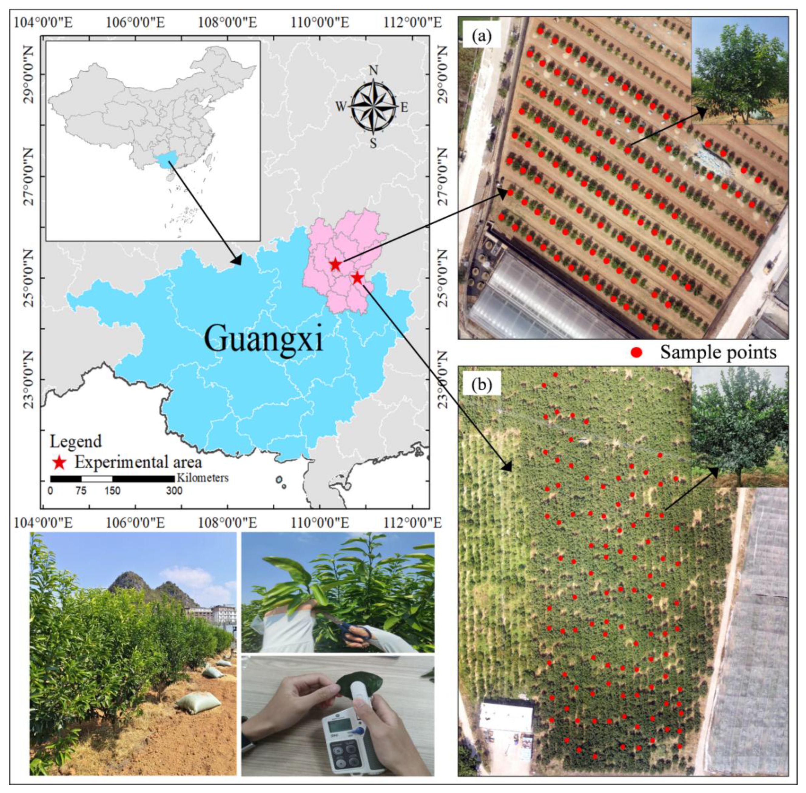
Figure 1. Study area. The geographical location of the study area is shown on the upper left, and the orthoimages of the experimental area and verification area are shown in (a) and (b), respectively, on the right. A schematic diagram of partial ground data collection is shown on the lower left.
Horticulturae 11 01223 g001
Figure 2. Measured spectra of the citrus fruit canopy in the experimental area.
Horticulturae 11 01223 g002
Figure 3. Optimizing the role of ALAs.
Horticulturae 11 01223 g003
Figure 4. Sensitivity analysis of several important parameters of the PROSAIL model in five multispectral bands.
Horticulturae 11 01223 g004
Figure 5. Comparison of the average values of the simulated spectral reflectivity and measured spectral reflectivity.
Horticulturae 11 01223 g005
Figure 6. Accuracy performance of hybrid inversion models with varying simulated-data ratios based on four machine learning methods ((a): PLSR, (b): GPR, (c): RFR, (d): SVR).
Horticulturae 11 01223 g006
Figure 7. ALAadj distribution box chart. (a) represents the experimental area, and (b) represents the verification area.
Horticulturae 11 01223 g007
Figure 8. Spectral response of parameters before and after ALA adjustment. (a) Spectral response with unadjusted ALA; (b) Spectral response after ALA adjustment.
Horticulturae 11 01223 g008
Figure 9. Comparison of performance between the ALA-unadjusted hybrid model and the ALAadj hybrid model under 4 kinds of machine learning. (a) PLSR-ALA-unadjusted; (b) GPR-ALA-unadjusted; (c) RFR-ALA-unadjusted; (d) SVR-ALA-unadjusted; (e) PLSR-ALAadj; (f) GPR-ALAadj; (g) RFR-ALAadj; (h) SVR-ALAadj.
Horticulturae 11 01223 g009
Figure 10. Comparison of performance between the ALA-unadjusted hybrid model and the ALAadj hybrid model in the validation area under the 4 machine learning methods. (a) PLSR-ALA-unadjusted; (b) GPR-ALA-unadjusted; (c) RFR-ALA-unadjusted; (d) SVR-ALA-unadjusted; (e) PLSR-ALAadj; (f) GPR-ALAadj; (g) RFR-ALAadj; (h) SVR-ALAadj.
Horticulturae 11 01223 g010
Table 1. Center wavelength and radiation correction coefficient of the UAV multispectral camera.
Multispectral BandsCenter Wavelength (Bandwidth)/nmRadiation Correction Coefficient
Blue450 ± 160.537
Green560 ± 160.538
Red650 ± 160.537
Red Edge730 ± 160.533
NIR840 ± 260.536
Table 2. Main measured parameter ranges.
ParameterRangeMean ValueUnit
SPAD[38.36, 73.86]58.89-
LCC[32.63, 99.30]65.26μg/cm2
LAI[1.02, 2.46]1.81-
CCC[51.23, 226.31]119.19μg/cm2
Table 3. Parameter ranges based on the PROSAIL model.
ModelParameterUnitRangeStep
PROSPECT 5-
4SAIL
Chlorophyll content (Cab)μg/cm232–1000.1
Leaf structure index (N)-1–20.1
Dry matter content (Cm)g/cm20.016-
Leaf water depth (Cw)cm0.02-
Carotenoid (Car)μg/cm225%Cab-
Brown pigments (Cb)-0-
Leaf area index (LAI)m2/m21–2.50.1
Soil coefficient (Psoil)-0.1–0.40.1
Hot spot parameter (Hspot)m/m0.1-
Average leaf angle (ALA)(°)10–805
Solar zenith angle (tts)(°)30-
Observe zenith angle (tto)(°)0-
Relative azimuth (psi)(°)0-
Table 4. Hyperparameter grids used for the four machine learning algorithms.
ModelHyperparameter Grids
PLSRn_components: [5, 10, 15, 20]
GPRkernel: [RBF, RBF + WhiteKernel]
alpha: [1 × 10⁻⁵, 1 × 10⁻³]
n_restarts_optimizer: [3, 5]
RFRn_estimators: [100, 200]
max_depth: [10, 20, None]
min_samples_split: [2, 5]
min_samples_leaf: [1, 2]
SVRkernel: [‘rbf’, ‘linear’]
C: [0.1, 1, 10]
epsilon: [0.1, 0.2]
gamma: [‘scale’, 0.01, 0.1]
Table 5. Dataset partitioning strategy.
Data SourceTotal SamplesTrainingTestingTraining ProportionTesting Proportion
Simulated Data4003505087.5%12.5%
Measured Data100505050%50%
Total50040010080%20%
Table 6. Changes in precision for the experimental area and verification area after ALA adjustment.
MethodHybrid Inversion ModelExperimental AreaValidation Area
R2RMSER2RMSE
PLSRALA-unadjusted0.62525.4650.67531.920
ALAadj0.78219.4670.72828.986
GPRALA-unadjusted0.68122.3430.64037.886
ALAadj0.74421.6760.71732.024
RFRALA-unadjusted0.72321.8660.72329.473
ALAadj0.82317.5210.74128.244
SVRALA-unadjusted0.71722.1310.74028.515
ALAadj0.81318.0070.84821.686
Disclaimer/Publisher’s Note: The statements, opinions and data contained in all publications are solely those of the individual author(s) and contributor(s) and not of MDPI and/or the editor(s). MDPI and/or the editor(s) disclaim responsibility for any injury to people or property resulting from any ideas, methods, instructions or products referred to in the content.