Abstract
Cerasus Humilis fruit is susceptible to rapid color changes post-harvest, which degrades its quality. This research utilized hyperspectral imaging technology to detect and visually analyze the soluble solid content (SSC) and firmness of the fruit, aiming to improve quality and achieve optimal pricing. Four maturity stages (color turning stage, coloring stage, maturity stage, and fully ripe stage) of Cerasus Humilis fruit were examined using hyperspectral images (895–1700 nm) alongside data collection on SSC and firmness. These samples were divided into a calibration set and a validation set with a ratio of 3:1 by sample set partitioning based on the joint X-Y distances (SPXY) method. The original spectral data was processed by a spectral preprocessing method. Multiple linear regression (MLR) and nonlinear least squares support vector machine (LS-SVM) detection models were established using feature wavelengths selected by the successive projections algorithm (SPA), competitive adaptive reweighted sampling (CARS), uninformative variable elimination (UVE), and two combined downscaling algorithms (UVE-SPA and UVE-CARS), respectively. For SSC and firmness detection, the best models were the SNV-SPA-LS-SVM model with 18 feature wavelengths and the original spectra-UVE-CARS-LS-SVM model with eight feature wavelengths, respectively. For SSC, the correlation coefficient of prediction (Rp) was 0.8526, the root mean square error of prediction (RMSEP) was 0.9703, and the residual prediction deviation (RPD) was 1.9017. For firmness, Rp was 0.7879, RMSEP was 1.1205, and RPD was 2.0221. Furthermore, the optimal model was employed to retrieve the distribution of SSC and firmness within Cerasus Humilis fruit. This retrieved information facilitated visual inspection, enabling a more intuitive and comprehensive assessment of SSC and firmness at each pixel level. These findings demonstrated the effectiveness of hyperspectral imaging technology for determining SSC and firmness in Cerasus Humilis fruit. This paves the way for online monitoring of fruit quality, ultimately facilitating timely harvesting.
1. Introduction
Cerasus Humilis (Prunus humilis Bunge) fruit is highly favored by most consumers due to its sweet and unique taste and rich nutrition. In evaluating Cerasus Humilis fruit quality, soluble solid content (SSC) and firmness are two important internal quality indicators. These properties are also two key indices for consumers to judge maturity and harvest time [1]. Detecting SSC and firmness indicators in Cerasus Humilis fruits is important for identifying ripeness, determining optimal harvest times, enhancing product value, and increasing fruit farmers’ income. Traditionally, the SSC of Cerasus Humilis fruit is tested by the refractometer method, which requires the fruit to be extruded into juice and then titrated, and the firmness is tested with the fruit texture analyzer (TA-xt-plus) [2]. Obviously, the methods for determining SSC and firmness of Cerasus Humilis fruit are different. Generally, to obtain a set of data that can actively reflect SSC and firmness of the whole sample, multiple measurements are necessary and the average value is regarded as the representative data. Though traditional testing methods ensure the accuracy of individual sample measurements, they are limited to sampling tests, which are inefficient and time-consuming, and cannot be performed for all samples. Tested samples are destroyed during the testing process and cannot be sold or consumed, resulting in many drawbacks. Additionally, due to the mutual influence of the two indicators, traditional chemical methods cannot simultaneously obtain both indicators [3]. This is cumbersome, time-consuming, and impractical for large-scale sample testing. Consequently, developing nondestructive techniques to determine the SSC and firmness of Cerasus Humilis fruits is essential.
In recent years, many nondestructive testing techniques have been used to evaluate fruit quality. Among them, visible and near infrared (Vis-NIR) spectral sensing technology can effectively evaluate the quality indicators in fruit (SSC, firmness, moisture content, etc.). However, this technique is a single point measurement for the sample, and can only obtain the spectral information of the sample, which cannot reflect the spatial information of the internal quality of the sample, and there is no visualization. Therefore, the technology has limitations. As a comparison, the hyperspectral imaging (HIS) technology combines the advantages of both spectroscopy and image, which can fulfill the task of visualization and has the advantages of simplicity, speed, non-destructiveness, and accuracy [4]. When the molecules in a substance transform from ground state to high energy level, vibrations containing hydrogen bonds (C-H, O-H, N-H, etc.) generate spectral information [5]. The position and intensity of spectral absorption peaks vary depending on the molecules and content in the material, leading to changes in spectral characteristics [6]. Therefore, combining hyperspectral imaging technology with chemometrics can analyze the component content of the material organic compounds (for soluble sugars and organic acids). In recent years, this technology has achieved significant success in fruit maturity detection and quality analysis [7,8,9]. For example, Benelli et al. [10] employed hyperspectral imaging to predict grape SSC during harvest, achieving a correlation coefficient of prediction (Rp) of 0.77 and a root mean square error of prediction (RMSEP) of 0.779 °Brix for their established partial least squares regression (PLSR) model. Similarly, Pullanagari et al. [11] utilized hyperspectral imaging with characteristic wavelengths to predict total soluble solid concentration (TSS) and flesh firmness (FF) in cherry fruit. Their Gaussian process regression (GPR) model yielded the best results with Rp values of 0.88 and 0.60 for TSS and firmness, respectively, along with RMSEP values of 0.43% and 0.38 N, and RPD values of 3.04 and 2.54. Additionally, recent studies have also shown that HSI is feasible for visualizing the distribution of internal quality in fruits, such as SSC and PH distribution of cherries, mandarins and kiwifruit [12,13,14], and firmness of peach [15]. Beyond these examples, research using hyperspectral imaging and chemometrics has shown promising results in maturity analysis and quality evaluation of blueberries, persimmons, bananas, and other fruits [16,17,18,19]. The above researches mainly focus on the prediction of single indicators of SSC and hardness during the sample maturity stages. However, there are few reports about detection of SSC and firmness in Cerasus Humilis fruits at different maturity stages by using HIS technology.
Therefore, the purpose of this study was to explore the application of hyperspectral imaging technology in SSC and firmness of Cerasus Humilis fruit at different maturity stages. In this study, fresh fruits at four maturity stages (color turning, coloring, maturity, and fully ripe) were collected, and their hyperspectral information was captured. We then established prediction models to relate spectral information to both SSC and firmness. The advantages and disadvantages of these models were compared to determine the optimal approach. Additionally, a visual analysis of fruit quality was performed. This research provides a theoretical foundation for developing an online testing system for the comprehensive quality evaluation of Cerasus Humilis fruit.
2. Materials and Methods
2.1. Samples
Following the established production protocols, the ripening process of Cerasus Humilis fruit was stratified into four distinct stages: color turning, coloring, maturity, and fully ripe. Figure 1 illustrates samples of Cerasus Humilis fruit at different maturity stages.

Figure 1.
Samples of Cerasus Humilis fruit at different maturity stages: (a) color turning stage; (b) coloring stage; (c) maturity stage; (d) fully ripe stage.
This study focused on “Nongda 6” Cerasus Humilis fruit harvested from the Jinzhong Agricultural High-Tech Industry Demonstration Zone planting base between July and August 2023. With the guidance of experienced fruit growers, 110 samples were collected at four specific points in the growth period: day 75 (color turning stage), day 85 (coloring stage), day 95 (maturity stage), and day 100 (fully ripe stage).
Following harvest, the samples were transported to the laboratory on the same day in a low-temperature preservation box. From the initial set of 110 samples per maturity stage, a total of 320 samples were meticulously selected based on stringent criteria. These criteria ensured the samples were free from defects, bruises, and diseases, and possessed relatively uniform shapes.
2.2. Hyperspectral Image Acquisition
2.2.1. Hyperspectral Imaging System
The hyperspectral imaging system used in this study is depicted in Figure 2. The system comprises an imaging spectrograph (GaiaSorter, Beijing, China), light sources, a data acquisition and processing unit, a CCD camera, electronically controlled mobile platforms, a computer, and a darkroom [20]. The system boasts a spectral range of 895–1700 nm (encompassing 254 wavelengths), with a spectral resolution of 5.0 nm, a wavelength interval of 3.19 nm, an effective slit length of 9.6 mm, an incident slit width of 30 μm, and a resolution of 320 × 256 pixels per image.
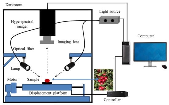
Figure 2.
Experiment platform of hyperspectral imaging system.
2.2.2. Image Acquisition and Calibration
To minimize temperature’s influence on the spectra and fruit quality, samples were equilibrated in the laboratory for 2 h at 25 °C and 40% RH before image collection. The hyperspectral imaging system was then warmed up for 30 min to ensure stability. For optimal image quality, we determined appropriate settings through repeated experiments. These included a sample-to-lens distance of 280 mm, a camera exposure time of 130 ms, and a mobile platform movement speed of 8.0 mm/s. Additionally, four tungsten halogen lamps positioned at a 45° angle above the sample reduced shadow effects.
A black and white correction was performed on the hyperspectral imaging system to compensate for the effects of light source fluctuations and camera dark current on the captured images [21]. Before measurements, the full black calibration image (IDark) was obtained with a black opaque cap completely covering the camera lens (0% reflectance), and a white reflection image (IWhite) was recorded by acquiring a spectral image from a Teflon whiteboard (99.99% reflectance). The corrected image IC was computed as follows:
where IRaw is the original hyperspectral image acquired, IWhite is a standard white reference image, and IDark is a dark reference image.
The ENVI 5.0 software was used to extract spectral data from regions of interest (ROIs) within the samples. For each fruit sample, a rectangular ROI measuring 60 × 70 pixels was manually extracted from the equatorial region. The average value of all spectral information within the ROI was then calculated to represent the corresponding reflected spectral value.
2.2.3. Chemical Analysis
Following the hyperspectral image acquisition of Cerasus Humilis fruit samples, a puncture test was conducted to assess firmness. The experiment utilized a Texture Analyzer (TMS-Pro, FTC, Washington, WA, USA) equipped with a 3 mm cylindrical probe. The force cell range was set to 100 N, loading speed to 0.3 mm/s, trigger force to 0.1 N, and maximum penetration depth to 10 mm. For firmness measurement, a 1 cm2 section of peel was removed from the upper, middle, and lower positions of the ROI for each sample. The firmness value at each position was measured, and the average of the three measurements was used as the overall firmness value for the sample. After firmness measurement, pulp was extracted from the same three locations for juice extraction. A PAL-1 digital refractometer was then used to measure the SSC of the juice. The average of the three SSC measurements was taken as the SSC value for the Cerasus Humilis fruit sample. Figure 3 presents the average values of these physical and chemical indicators for Cerasus Humilis fruits at different maturity stages.
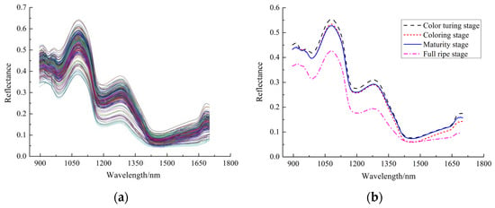
Figure 3.
Raw reflectance spectra of Cerasus Humilis fruit samples at different maturity stages: (a) original spectral curve; (b) average spectrum.
2.3. Data Processing
2.3.1. Sample Partitioning
Prior to establishing a prediction model, the samples were divided into two sets: a calibration set and a prediction set. The model was trained using the calibration set data, followed by performance testing on the prediction set data. This sample division employed the Sample Set Partitioning Based on Joint X-Y Distance (SPXY) algorithm. The algorithm used spectral values as the X variable and physicochemical indicators (SSC and firmness) as the Y variable, achieving a 3:1 ratio between the calibration and prediction sets [22]. To assess the validity of this division, the maximum, minimum, mean, and standard deviation of spectral data were calculated for both the calibration and prediction sets.
2.3.2. Spectral Preprocessing
The collected spectral information comprised not only the internal structure and component information of the tested sample, but also interference caused by various factors such as light scattering, sample heterogeneity, temperature fluctuations, and instrument noise [23]. To enhance model stability, preprocessing the original spectrum is crucial. This study employed five spectral preprocessing methods: Savitzky–Golay (S-G), Standard Normal Variate (SNV), Multiplicative Scatter Correction (MSC), Baseline Correction (BC), and De-trending (De-T). Subsequently, Partial Least Squares (PLS) regression was used to evaluate the performance of the data processed with these different methods.
2.3.3. Selection Methods of Characteristic Wavelengths
The full spectrum, encompassing 254 wavelength variables, presents a challenge due to potential information redundancy. A large number of collinear wavelengths can contribute to this redundancy, which in turn increases computational load, reduces modeling efficiency, and ultimately affects model performance. To address these limitations and streamline the modeling process, enhance computational speed, and improve prediction accuracy, dimensionality reduction of the raw spectral data becomes necessary. This study employed several feature selection methods for dimensionality reduction: the Successive Projections Algorithm (SPA), Competitive Adaptive Reweighted Sampling (CARS), and Uninformative Variable Elimination (UVE). Additionally, combined approaches, including UVE-CARS and UVE-SPA, were utilized. These methods aim to reduce the dimensionality of the spectral data by selecting characteristic wavelengths that effectively capture the essential information from the full spectrum.
The SPA is a forward loop feature selection method. It effectively filters out irrelevant information, significantly reduces the collinearity effect between data points, and utilizes root mean square error (RMSE) for evaluation [24]. CARS is another effective method for wavelength selection. It leverages the principles of “survival of the fittest” and regression coefficients. First, a PLS model was used to identify wavelengths with large regression coefficients. Then, 10-fold cross-validation was employed to select the wavelength subset with the smallest RMSE [25]. UVE also selected wavelengths based on PLS regression coefficients. This method added a specific number of random variables to the spectral matrix. Subsequently, a PLS model was established through cross-validation. Finally, the ratio of regression coefficient to standard deviation was calculated to identify and select effective spectral information [20].
2.3.4. Models Establishment
Partial least squares regression offers several advantages over traditional methods like set-correlation analysis, multiple linear regression (MLR), and principal component analysis (PCA) [13]. PLSR is a widely used quantitative analysis technique based on multivariate linear modeling. It performs curve fitting by minimizing the sum of squared deviations between predicted and actual values. This method effectively utilizes both spectral information from samples and their physicochemical properties to create an optimal calibration model. PLSR is used to search for potential linear combinations of wavelength variables (X) and chemical composition (Y). Its expression is as follows:
where and are the regression coefficient matrix and regression residual matrix, respectively.
MLR, a common modeling approach, establishes relationships between dependent and multiple independent variables [26]. While MLR boasts a simple algorithm and easy interpretation, it suffers from vulnerabilities to collinearity (high correlation) between variables. Additionally, the number of variables in an MLR model must be less than the number of samples for proper function. The equation is as follows:
where represents the component content of the tested sample, represents the constant, represents the regression coefficient, represents the spectral data at different wavelength bands, and represents the regression bias.
Least squares support vector machine (LS-SVM) represents an improvement over traditional support vector machines (SVM). LS-SVM effectively addresses both linear and non-linear problems by finding linear equations [27]. It achieves this by solving a set of linear equations with equality constraints, as opposed to the complex quadratic optimization problems encountered in traditional SVMs. Consequently, LS-SVM boasts improved computational efficiency and enhanced model prediction capabilities. The choice of kernel function directly determines the performance of the LS-SVM model. There are many types of kernel functions (such as linear, polynomial, and radial basis function (RBF)), among which the RBF has the characteristics of low complexity and few parameters. Therefore, RBF was chosen as the kernel function of LS-SVM in this study. The grid search algorithm and leave-one-out cross validation (LOOCV) method were used to determine the optimal parameters of gamma (γ) and sigma2 (σ2) of the RBF kernel [13]. The LS-SVM model can be expressed as:
where is the kernel function, is the input vector, is the Langland multiplier (also known as the support vector), and is the model bias.
3. Results and Discussion
3.1. Spectral Analysis
Following the removal of head and tail noise, spectral feature analysis was conducted on the 230 bands within the 945–1675 nm range. This analysis yielded the spectral curves and average spectral curves for all Cerasus Humilis fruit samples, as presented in Figure 3.
Figure 3 illustrates a degree of spectral overlap between samples from distinct maturity stages, although the overall spectral curve trends exhibit significant similarity. The spectra in Figure 3a display prominent absorption peaks at 980 nm, 1195 nm, and 1460 nm, attributed to the second overtone of O-H in water and carbohydrates (around 980 nm and 1195 nm) [28,29] and the first overtone of the O-H bond (near 1460 nm), respectively. As depicted in Figure 3b, the average spectral curves for the various maturity stages (color turning, coloring, maturity, and fully ripe) demonstrated generally consistent trends. However, the spectral reflectance of the samples exhibited a significant difference as the maturity period progressed, with the fully ripe stage exhibiting the lowest reflectance values. Notably, the range of 1180–1300 nm revealed a relatively substantial difference in fruit reflectivity, which then tended to decrease gradually. This observation might be linked to the alterations in the chemical composition of Cerasus Humilis fruits at different maturity stages. Nevertheless, it was not feasible to isolate the content of a specific compound based solely on these wavelengths, as each wavelength reflects intricate compositional information. Consequently, data analysis methods have become crucial for uncovering the underlying relationships between spectra and the measured physicochemical properties (SSC and firmness).
3.2. Statistics of SSC and Firmness
Figure 4 reveals significant differences in SSC and firmness across the various maturity stages of Cerasus Humilis fruit, reflecting the changes in internal quality during fruit development. The SSC content exhibits a continuous upward trend throughout the maturity stages, reaching a maximum value of 17.93 °Brix at the fully ripe stage. Conversely, the firmness value displays a continuous decline throughout development. The highest firmness (13.69 kg/cm2) is observed during the color turning stage, while the fully ripe stage exhibits the lowest firmness (9.12 kg/cm2). These findings align with the established research on the internal physical and chemical changes in fruits at different maturity stages.
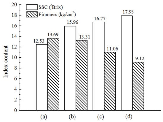
Figure 4.
Average physical and chemical indexes of Cerasus Humilis fruit at different stages: (a) color turning stage; (b) coloring stage; (c) maturity stage; (d) fully ripe stage.
All Cerasus Humilis fruit samples were divided into calibration set and prediction set based on SPXY method mentioned in Section 2.3.1. Table 1 presents the statistical results of this sample set division. As can been seen, the SSC in the calibration set ranged from 9.24 to 18.5 °Brix with an average of 14.65 °Brix. Firmness values in the calibration set ranged from 5.86 to 16.64 kg/cm2 with an average of 11.45 kg/cm2. Similarly, the prediction set exhibited an SSC range of 11.32 to 18.17 °Brix with an average of 14.91 °Brix, and a firmness range of 7.61 to 16.53 kg/cm2 with an average of 12.45 kg/cm2. This distribution achieved through the SPXY algorithm ensured that the calibration set encompasses the range of SSC and firmness values present in the prediction set. Those properties were very important to establish a robust and stable prediction model.

Table 1.
Statistical for the SSC and firmness of Cerasus Humilis fruit.
3.3. Spectral Pretreatment
Given that the number of latent variables (Lvs) in PLSR significantly impacts model performance, this study employed 10-fold cross validation to determine the optimal Lvs for PLSR modeling of both SSC and firmness. Spectral data preprocessed using each method were then used as input variables for PLSR modeling, establishing corresponding prediction models for each quality parameter. Table 2 presents the PLSR modeling results obtained with different pretreatment methods.

Table 2.
Results of full wavelength PLSR model based on different preprocessing methods.
Table 2 reveals that for the SSC index of Cerasus Humilis fruit, the PLSR model established using SNV pretreatment on the original spectra achieved the best prediction performance compared to models based on other preprocessing methods. This model yielded the highest correlation coefficients (Rc = 0.7709, Rp = 0.8596), the highest RPD value (1.8705), and the lowest root mean square errors for calibration and prediction (1.1963 and 0.9865, respectively).
Interestingly, for the firmness index, the PLSR model based on the original spectra outperformed models based on all five preprocessing methods (S-G, SNV, MSC, BC, and DE-T). The model using the original spectra exhibited increased correlation coefficients (Rc = 0.6737, Rp = 0.7836), decreased RMSEC (1.4674) and RMSEP (1.2536) values, and the maximum RPD value (1.8074). These results suggest that, for firmness prediction, the original spectra contained more relevant information compared to the preprocessed data. It is highly conceivable that some preprocessing algorithms might have eliminated noise or scattering effects that were actually correlated with firmness.
3.4. Effective Wavelength Selection
3.4.1. Successive Projections Algorithm
In the SSC and firmness characteristic wavelength screening of Cerasus Humilis fruit, the minimum and maximum values of the wavelength variable were 2 and 30, respectively. Figure 5 illustrates the distribution of RMSE for the SPA algorithm with different numbers of selected variables. The RMSE values reached a minimum at 18 and 4 wavelength variables, being 1.2176 and 1.9416, respectively. Figure 6 depicts the distribution of the effective wavelengths chosen by SPA for predicting SSC and firmness. For SSC prediction, the 18 characteristic wavelengths were 1208, 1514, 1558, 1177, 1004, 1457, 1157, 1657, 1663, 956, 1014, 1402, 976, 1135, 1596, 947, 1393, and 1084 nm, respectively. These wavelengths accounted for approximately 3.91% of the total analyzed wavelengths, with the importance of each wavelength decreasing sequentially. For firmness prediction, the four characteristic wavelengths were 1100, 1202, 1364, and 1007 nm, constituting only 1.74% of the total wavelengths.
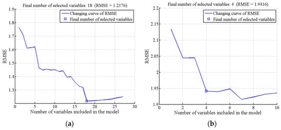
Figure 5.
RMSE plots obtained by SPA: (a) SSC; (b) firmness.
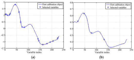
Figure 6.
Optimal characteristic wavelength distribution selected by SPA: (a) SSC; (b) firmness.
3.4.2. Competitive Adaptive Reweighted Sampling
The CARS algorithm employed 50 Monte Carlo sampling iterations and a 5-fold cross-validation method for characteristic wavelength selection. Figure 7 illustrates the selection process. Figure 7a–c depict the trends observed during each CARS run as the number of Monte Carlo samples increased. These trends included the number of sampled variables (a), the RMSECV values (b), and the regression paths for each variable (c). In Figure 7c, each curve represents the change in regression coefficients for a spectral variable as the number of sampling runs increases. The vertical line marked “*” indicates the point where the RMSECV reaches a minimum value (1.1355) with 33 sampling runs. At this minimum, 10 characteristic wavelengths were selected: 960, 1081, 1119, 1154, 1215, 1298, 1383, 1622, 1625, and 1672 nm, constituting approximately 4.35% of the total analyzed wavelengths. Similarly, for firmness prediction, the minimum RMSECV value (1.9134) was reached with 31 sampling iterations. This resulted in the selection of eight characteristic wavelengths: 963, 1103, 1202, 1205, 1208, 1272, 1377, and 1520 nm, representing 3.48% of the total wavelengths.
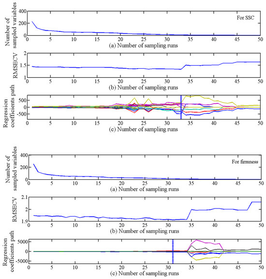
Figure 7.
Process of selecting wavelength variables by CARS for SSC and firmness: (a) number of sampled variables; (b) variation of RMSECV under different sampling times; (c) regression coefficients of each wavelength variable.
3.4.3. Uninformative Variable Elimination
Taking the SSC feature wavelength selection of Cerasus Humilis fruit as an example, the UVE algorithm was used to eliminate the uninformative variables from the original 230 wavelengths. When using a five-fold cross-validation scheme and setting the number of principal components to 12, the minimum RMSECV value obtained was 1.3036, as illustrated in Figure 8a.
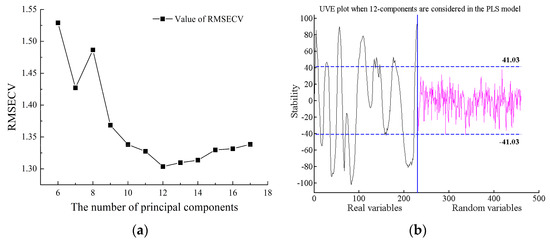
Figure 8.
Process of selecting wavelength variables for SSC by UVE: (a) RMSECV distribution with a different number of principal components; (b) stability distribution of characteristic wavelength.
Figure 8b depicts the stability distribution results of the UVE algorithm for characteristic wavelength selection with 12 principal components. The curves on the left side of the vertical line represent the original 230 wavelength variables, while those on the right represent randomly introduced variables. The upper and lower dashed lines indicate the selection threshold for random variables (±41.03), set at 99% of the maximum stability value of the random variable. Information exceeding the absolute value of this threshold was considered valid. In simpler terms, information above and below the dashed lines was considered useful, while information between the lines was deemed irrelevant. Consequently, variables exceeding the threshold were preserved for further model analysis. This process resulted in the selection of 129 characteristic wavelengths, constituting approximately 56.09% of the total wavelengths.
Similarly, the selection of characteristic wavelengths for firmness in Cerasus Humilis fruit yielded a minimum RMSECV value of 1.9097 with 10 principal components. The selection threshold in this case was ±35.96, leading to the extraction of 53 characteristic wavelengths, representing 23.04% of the total wavelengths. The analysis results are presented in Figure 9.
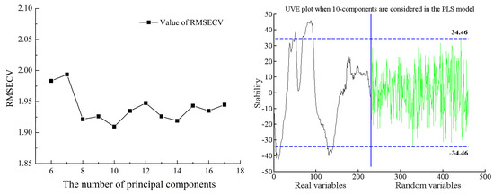
Figure 9.
Process of selecting wavelength variables for firmness by UVE.
3.4.4. Secondary Effective Wavelength Selection
Dimensionality reduction using the three aforementioned methods (SPA, CARS, UVE) successfully eliminated irrelevant information and reduced the wavelength dimension. While the UVE algorithm yielded a higher number of characteristic wavelengths compared to SPA and CARS, it might introduce issues with redundant information and multicollinearity in the spectral data. Conversely, SPA and CARS algorithms bring the advantage of eliminating multicollinearity among spectral variables, effectively addressing the limitations of UVE. Therefore, SPA and CARS were employed for further screening.
For SSC prediction, the UVE-SPA algorithm was used to select characteristic wavelengths. The number of selected wavelengths was determined based on the RMSE value. Figure 10 illustrates the trend of RMSE with different variable numbers. As the number of variables increased, RMSE exhibited a decreasing trend. The minimum RMSE value (1.2518) was achieved with 15 variables (marked in blue squares). These 15 characteristic wavelengths were 1218, 1189, 969, 1151, 1453, 1577, 995, 1110, 1367, 1129, 953, 960, 1409, 1596, and 1647 nm, representing approximately 6.52% of the total wavelengths. Additionally, the UVE-CARS algorithm was used for characteristic wavelength selection. The minimum RMSECV value (1.3406) was obtained with 31 sampling runs. Figure 11 presents the results of effective wavelength selection. Ten characteristic wavelengths were identified: 995, 1036, 1075, 1081, 1119, 1122, 1151, 1208, 1383, and 1628 nm, constituting 4.35% of the original spectral wavelengths.
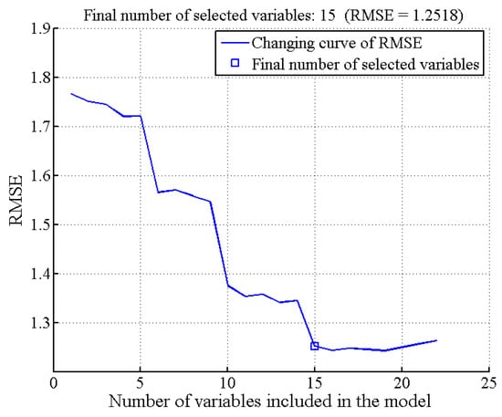
Figure 10.
Characteristic wavelength selection results by UVE-SPA.
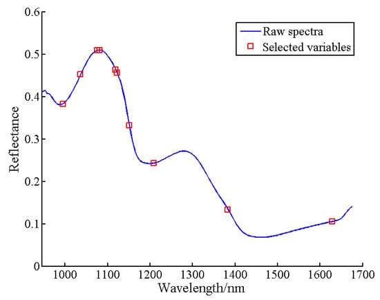
Figure 11.
Distribution of the optimal characteristic wavelength selected by UVE-CARS.
Following the same approach, the UVE-SPA and UVE-CARS algorithms selected four and eight characteristic wavelengths for firmness prediction, respectively. These wavelengths accounted for 1.74% and 3.48% of the original spectral data, as detailed in Table 3.

Table 3.
Characteristic wavelengths selected by secondary dimension reduction models.
3.5. Model Analysis
3.5.1. MLR Model
Table 4 demonstrates the effectiveness of dimensionality reduction using different characteristic wavelength extraction methods on the original spectral data. For the SSC index of Cerasus Humilis fruit, the UVE-SPA and UVE-CARS methods further reduced the number of characteristic wavelengths compared to other methods, leading to a significant improvement in model prediction performance. Notably, the MLR model established with UVE-SPA wavelengths achieved the best results (Rp = 0.8326, RMSEP = 0.9913, RPD = 1.8614). This suggested that the combined UVE-SPA approach effectively eliminated redundant and multicollinear variable information, extracting the most relevant characteristic wavelengths for prediction. Additionally, the UVE-SPA-MLR model benefited from a lower number of variables (only 15), significantly reducing modeling time.

Table 4.
Results of MLR model based on different characteristic wavelength extraction methods.
For firmness prediction models, the UVE-SPA-MLR model exhibited the weakest performance (Rp = 0.6694, RMSEP = 1.4005, RPD = 1.6179), given that the SPA algorithm, during secondary screening, excluded some valuable spectral information identified by the UVE algorithm. In contrast, the CARS-MLR model achieved better results (Rp = 0.7287, RMSEP = 1.2926, RPD = 1.7529). However, the UVE-CARS-MLR model emerged as the best model for firmness prediction, with Rp = 0.7629, RMSEP = 1.2545, and RPD = 1.8061. Furthermore, UVE-CARS identified only eight characteristic wavelengths (3.48% of the total), demonstrating its efficiency in variable selection.
The MLR prediction model for the SSC index of Cerasus Humilis fruit based on UVE-SPA optimal characteristic wavelength was as follows:
The MLR prediction model for the firmness index of Cerasus Humilis fruit based on UVE-CARS optimal characteristic wavelength was as follows:
3.5.2. LS-SVM Model
To investigate whether a nonlinear model outperforms the linear model in predicting the internal quality parameters of Cerasus Humilis fruit. Here, we established nonlinear LS-SVM prediction models for both SSC and firmness of Cerasus Humilis fruit. The predicted results from these LS-SVM models with different variables are presented in Table 5.

Table 5.
Results of LS-SVM model based on different characteristic wavelength.
Table 5 demonstrates that, for the SSC index of Cerasus Humilis fruit, LS-SVM models based on all five characteristic wavelength extraction methods (SPA, CARS, UVE, UVE-SPA, and UVE-CARS) achieve consistently higher correlation coefficients (Rc and Rp) and lower root mean square errors (RMSEC and RMSEP). These findings indicated a strong overall prediction performance for the LS-SVM model across the various wavelength extraction techniques. The CARS-LS-SVM and UVE-CARS-LS-SVM models exhibited similar predictive capabilities, suggesting that both CARS and UVE-CARS were effective in extracting relevant variable information. While the SPA-LS-SVM model achieved comparable accuracy to the UVE-LS-SVM and UVE-SPA-LS-SVM models, it offered a distinct advantage: the SPA method eliminated the need for secondary feature wavelength screening (requiring only 18 variables). This translated to significant time savings and improved model fitting efficiency. Therefore, considering a balance between accuracy, stability, and model complexity, the SPA-LS-SVM model emerged as the optimal choice for predicting SSC in Cerasus Humilis fruit.
For the firmness index of Cerasus Humilis fruit, the LS-SVM model based on UVE-SPA characteristic wavelengths exhibited the weakest performance, achieving Rp of 0.6926, RMSEP of 1.3060, and RPD of 1.7349. This suggested that, during the secondary screening, the SPA algorithm might have eliminated some valuable spectral information identified by the UVE algorithm. The SPA-LS-SVM model achieved slightly better results (Rp = 0.7392, RMSEP = 1.2879, RPD = 1.7593). Notably, the CARS-LS-SVM model demonstrated superior performance (Rp = 0.7635, RMSEP = 1.1889, RPD = 1.9058). The UVE-LS-SVM model yielded results (Rc = 0.7353, RMSEC = 1.3390, Rp = 0.7775, RMSEP = 1.1333, RPD = 1.9993) slightly lower than the UVE-CARS-LS-SVM model (Rc = 0.7283, RMSEC = 1.3578, Rp = 0.7879, RMSEP = 1.1205, RPD = 2.0221). However, the UVE-CARS-LS-SVM model achieved this performance with a significantly smaller number of variables (only eight). In conclusion, among all LS-SVM models, the UVE-CARS-LS-SVM model emerged as the one with the best prediction performance for firmness.
3.5.3. Model Comparison and Analysis
Table 6 demonstrates that the established nonlinear LS-SVM models outperformed their linear MLR counterparts in predicting both SSC and firmness of Cerasus Humilis fruit. Notably, the SPA-LS-SVM and UVE-CARS-LS-SVM models emerged as the optimal models for SSC and firmness prediction, respectively. The LS-SVM model achieved exceptional prediction performance for firmness (RPD > 2.0), surpassing the performance for SSC. Nevertheless, the SSC prediction model’s performance also meets acceptable standards. These findings collectively indicate that the nonlinear LS-SVM models yielded superior prediction accuracy and stability compared to the linear MLR models. The predicted and measured SSC and firmness values of Cerasus Humilis fruit by the optimal LS-SVM model were shown in Figure 12. The solid line is a regression line that corresponds to the ideal correlation between measured values and predicted values. From Figure 12, it can be seen that the predicted values were basically close to the corresponding actual values for both calibration and prediction sets.

Table 6.
Prediction results of best MLR and LS-SVM models for SSC and firmness values of fruit.
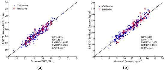
Figure 12.
Scatter plots of the measured and predicted various indexes of SSC and firmness of Cerasus Humilis fruit based on the optimal model: (a) SPA-LS-SVM model predicts SSC results; (b) UVE-CARS- LS-SVM model predicts firmness results.
As shown in Figure 13, the distribution of characteristic bands of SSC and firmness in the spectral curve. It can be seen that the specific characteristics of the first region (945–1100) may be caused by the vibration of hydrogen groups (O-H and N-H), which was the third overtone region of O-H and absorption band of water. The fruit contains acidic compounds, which usually contain hydrogen groups. However, the absorption peaks in the second region (1100–1210) and the third region (1220–1600) are mainly caused by vibrations of C=O (1160 nm) and C-H (1170 nm, 1194 nm), and these two chemical bonds are commonly present in soluble sugars, which are the major components of SSC [12]. In this figure, each triangle and pentagram marks the position of a feature band in the spectral curve.
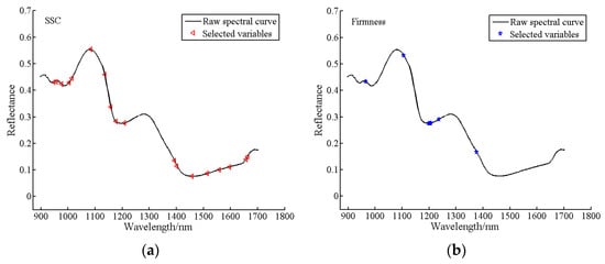
Figure 13.
The distribution of characteristic bands in spectral curves: (a) SSC; (b) firmness.
3.6. Visualization of SSC and Firmness Distribution
Distribution maps of SSC and firmness play a valuable role in online detection. This study employed SPA-LS-SVM and UVE-CARS-LS-SVM models to estimate the SSC and firmness values for each pixel within Cerasus Humilis fruit samples. Pseudo-color image processing technology was then utilized to generate the corresponding distribution maps. In these maps (Figure 14), different colors and shades represent varying magnitudes of SSC and firmness across the fruit at different maturity stages.
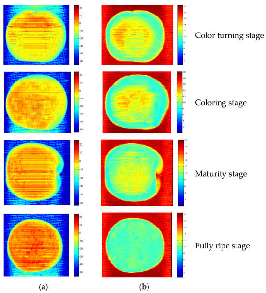
Figure 14.
SSC and firmness distribution map of Cerasus Humilis fruit in different maturities: (a) SSC; (b) firmness.
Figure 14a depicts the SSC distribution during the fully ripe stage. The fruit appeared predominantly dark red, covering approximately 98% of the area, indicating an SSC concentration in the range of 17–20 °Brix. Compared to the fully ripe stage, the color density in Figure 14a gradually changed from red to yellow throughout the maturity, coloring, and color turning stages, reflecting a decrease in SSC.
Figure 14b shows the firmness distribution at the ripe stage. Here, the Cerasus Humilis fruit appeared primarily light green, covering almost the entire area, with firmness concentrated in the 9–10 kg/cm2 range. In the coloring and ripening stages, the fruit color transitioned from dark yellow to light green, with the yellow pixels becoming lighter. This change suggested a gradual decrease in firmness value. Notably, the blue and red areas outside the fruit region in the SSC and firmness images, respectively, represented the background used for data collection.
The visualization of the distribution maps demonstrated an increase in SSC and a decrease in firmness as the ripening stage progressed. Furthermore, the maps revealed an uneven distribution of SSC and firmness across different locations within each sample. This unevenness likely stemmed from variations in the rates of compound conversion occurring within the Cerasus Humilis fruit during the ripening process. Therefore, SSC and firmness visualization distribution maps can be a valuable tool for consumers, enabling them to rapidly assess the quality of Cerasus Humilis fruit. This technology holds promise for online quality detection of Cerasus Humilis fruit.
4. Discussion
This study investigated the use of hyperspectral data for non-destructive, accurate, and rapid identification of SSC and firmness in Cerasus Humilis fruit. The study revealed a clear advantage of the LS-SVM model over the MLR model in predicting SSC and firmness under similar conditions. This finding suggested a potentially non-linear relationship between the spectral range of 895–1700 nm and the fruit’s SSC and firmness. The superiority of LS-SVM compared to other models has been demonstrated in previous studies. The selected characteristic wavelengths were found to be distributed throughout the entire band, indicating that SSC is related to moisture (947, 956, and 976 nm) as well as carbohydrates such as soluble sugars and pectin (1104, 1014, 1084, 1135, 1157, 1177, 1208, 1393, 1402, 1457, 1514, 1558, and 1596 nm). The following studies draw the same conclusion. For example, Zhang et al. [30] employed hyperspectral imaging to measure the SSC of apples, achieving an optimal model (CARS-SPA-LS-SVR) with Rp = 0.917 and RMSEP = 0.453 °Brix. Similarly, Shao et al. [31] used Vis-NIR hyperspectral imaging to detect the SSC of winter jujube at different maturity stages, finding the SPA-LS-SVM model to be the most effective. It should be borne in mind that prediction results can vary depending on the research subject and specific conditions. At present, some research reports have conducted visualization studies on SSC, firmness, and anthocyanins content in fruit. For example, Li et al. [32] visualized anthocyanin content in mulberry fruit by using Vis-NIR hyperspectral imaging. Yang et al. [33] used near infrared hyperspectral imaging to visualize the SSC distribution in peaches. Similar studies include seed moisture content [34] and starch content of potato [35]. However, unlike most previous studies that focused on a single quality parameter, in this study, both the distribution of SSC and firmness were visually analyzed within Cerasus Humilis fruit at different maturity stages. This visualization capability provides valuable insights for consumers, allowing them to predict the internal quality of the fruit. To sum up, the feasibility and effectiveness of HSI for the determination of SSC and firmness in Cerasus Humilis fruit was confirmed.
5. Conclusions
This study explored the feasibility of determining the SSC and firmness in Cerasus Humilis fruit at different maturity stages by using hyperspectral imaging combined with chemometrics algorithms. The original spectral data were preprocessed. Five effective wavelength selection algorithms were employed to extract characteristic wavelengths. Subsequently, both linear MLR and nonlinear LS-SVM prediction models were established. The results indicate that the optimal model for SSC prediction was SPA-LS-SVM (Rp = 0.8526, RMSEP = 0.9703, RPD = 1.9017), while the optimal model for firmness prediction was UVE-CARS-LS-SVM (Rp = 0.7879, RMSEP = 1.1205, RPD = 2.0221). Finally, a color distribution map was constructed and visualized to represent the SSC and firmness of Cerasus Humilis fruit. The study indicates that the using of the hyperspectral imaging technology combined with chemometric algorithms provides a nondestructive determine method for determining the SSC and firmness of Cerasus Humilis fruit, evidencing the prospect of applying HSI to evaluating internal quality of fruits.
The method proposed in this study realizes the SSC and firmness detection of different maturity stages Cerasus Humilis fruits, which could be very helpful for real-time monitoring of Cerasus Humilis fruits quality by spectral imaging technique. It provides theoretical support for the development of portable equipment and on-line testing equipment. Even so, it should be noted that similar size and intact samples of Cerasus Humilis fruits were used at different maturity stages in this study. In practice, however, fruit quality is influenced by various factors, such as variety, origin, size, defects (cracks, pests, bruises, and rust spots), temperature, and humidity, etc. In future studies, the influence of the above factors should be considered to improve the robustness (universality) of the model, while adding new model algorithms (such as convolutional neural network). At the same time, the production line of Cerasus Humilis fruits quality detection will be developed and optimized based on hyperspectral imaging technology.
Author Contributions
Conceptualization, B.W.; methodology, B.W. and L.L.; software, B.W. and L.L.; data curation, B.W. and L.L.; writing—original draft, B.W.; writing—review and editing, B.W., S.Z., H.Y. and L.L. All authors have read and agreed to the published version of the manuscript.
Funding
This research was Supported by Fundamental Research Program of Shanxi Province (Grant NO. 202303021212120, No. 202203021212426). “Introduction of Talents and Scientific Research Initiation Project” of Shanxi Agricultural University (Project No. 2023BQ42, No. 2023BQ114).
Data Availability Statement
Data are contained within the article.
Acknowledgments
The authors thank the editor and anonymous reviewers for providing helpful suggestions for improving the quality of this manuscript. We thank Home for Researchers editorial team (www.home-for-researchers.com) for language editing service.
Conflicts of Interest
The authors declare no conflicts of interest.
References
- Wang, B.; Yang, H.; Zhang, S.; Li, L. Detection of defective features in cerasus humilis fruit based on hyperspectral imaging technology. Appl. Sci. 2023, 13, 3279. [Google Scholar] [CrossRef]
- Li, L.; Lu, L.M.; Zhao, X.H.; Hu, D.Y.; Tang, T.Y.; Tang, Y.L. Nondestructive detection of tomato quality based on multiregion combination model. J. Food Process Eng. 2022, 45, e14100. [Google Scholar] [CrossRef]
- De Brito, A.A.; Campos, F.; dos Reis Nascimento, A.; Damiani, C.; da Silva, F.A.; de Almeida Teixeira, G.H.; Júnior, L.C.C. Non-destructive determination of color, titratable acidity, and dry matter in intact tomatoes using a portable Vis-NIR spectrometer. J. Food Compos. Anal. 2022, 107, 104288. [Google Scholar] [CrossRef]
- Shang, Y.; Bao, L.; Bi, H.; Guan, S.; Xu, J.; Gu, Y.; Zhao, C. Authenticity discrimination and adulteration level detection of camellia seed oil via hyperspectral imaging technology. Food Anal. Methods 2024, 17, 450–463. [Google Scholar] [CrossRef]
- Sun, J.; Shi, X.; Zhang, H.; Xia, L.; Guo, Y.; Sun, X. Detection of moisture content in peanut kernels using hyperspectral imaging technology coupled with chemometrics. J. Food Process Eng. 2019, 42, e13263. [Google Scholar] [CrossRef]
- Baiano, A. Applications of hyperspectral imaging for quality assessment of liquid based and semi-liquid food products: A review. J. Food Eng. 2017, 214, 10–15. [Google Scholar] [CrossRef]
- Sun, H.; Zhang, S.; Ren, R.; Xue, J.; Zhao, H. Detection of soluble solids content in different cultivated fresh jujubes based on variable optimization and model update. Foods 2022, 11, 2522. [Google Scholar] [CrossRef] [PubMed]
- Wang, Z.; Wu, S.; Zuo, C.; Jiang, M.; Song, J.; Ding, F.; Pan, L. Exploring the variability and heterogeneity of apple firmness using visible and near-infrared hyperspectral imaging. LWT-Food Sci. Technol. 2024, 192, 115704. [Google Scholar] [CrossRef]
- Feng, S.; Shang, J.; Tan, T.; Wen, Q.; Meng, Q. Nondestructive quality assessment and maturity classification of loquats based on hyperspectral imaging. Sci. Rep. 2023, 13, 13189. [Google Scholar] [CrossRef] [PubMed]
- Benelli, A.; Cevoli, C.; Ragni, L.; Fabbri, A. In-field and non-destructive monitoring of grapes maturity by hyperspectral imaging. Biosyst. Eng. 2021, 207, 59–67. [Google Scholar] [CrossRef]
- Pullanagari, R.R.; Li, M. Uncertainty assessment for firmness and total soluble solids of sweet cherries using hyperspectral imaging and multivariate statistics. J. Food Eng. 2021, 289, 110177. [Google Scholar] [CrossRef]
- Li, X.; Wei, Y.; Xu, J.; Feng, X.; Wu, F.; Zhou, R.; He, Y. SSC and pH for sweet assessment and maturity classification of harvested cherry fruit based on NIR hyperspectral imaging technology. Postharvest Biol. Technol. 2018, 143, 112–118. [Google Scholar] [CrossRef]
- Luo, W.; Zhang, J.; Liu, S.; Huang, H.; Zhan, B.; Fan, G.; Zhang, H. Prediction of soluble solid content in Nanfeng mandarin by combining hyperspectral imaging and effective wavelength selection. J. Food Compos. Anal. 2024, 126, 105939. [Google Scholar] [CrossRef]
- Ma, T.; Xia, Y.; Inagaki, T.; Tsuchikawa, S. Non-destructive and fast method of mapping the distribution of the soluble solids content and pH in kiwifruit using object rotation near-infrared hyperspectral imaging approach. Postharvest Biol. Technol. 2021, 174, 111440. [Google Scholar] [CrossRef]
- Xu, L.; Chen, M.; Wang, Y.; Chen, X.; Lei, X. Study on non-destructive detection method of kiwifruit sugar content based on hyperspectral imaging technology. Spectrosc. Spectr. Anal. 2021, 41, 2188–2195. [Google Scholar]
- Choi, J.Y.; Kim, J.; Jeong, S.; Kim, M.; Park, S.; Moon, K.D. Hyperspectral imaging technigue for monitoring moisture content of blueberry during the drying process. Korean J. Food Preserv. 2021, 28, 445–455. [Google Scholar] [CrossRef]
- Baek, M.W.; Tilahun, S. Prediction of tannin content and quality parameters in astringent persimmons from visible and near-infrared spectroscopy. Front. Plant Sci. 2023, 14, 1260644. [Google Scholar] [CrossRef]
- Chu, X.; Miao, P.; Zhang, K.; Wei, H.; Fu, H.; Liu, H.; Ma, Z. Green banana maturity classification and quality evaluation using hyperspectral imaging. Agriculture 2022, 12, 530. [Google Scholar] [CrossRef]
- Taghinezhad, E.; Rasooli Sharabiani, V.; Shahiri, M.; Moinfar, A.; Szumny, A. Predicting quality properties of pears during storage using hyper spectral imaging system. Agriculture 2023, 13, 1913. [Google Scholar] [CrossRef]
- Wang, B.; He, J.; Zhang, S.; Li, L. Nondestructive prediction and visualization of total flavonoids content in Cerasus Humilis fruit during storage periods based on hyperspectral imaging technique. J. Food Process Eng. 2021, 44, e13807. [Google Scholar] [CrossRef]
- Guo, Z.; Zhao, C.; Huang, W. Intensity correction of visualized prediction for sugar content in apple using hyperspectral imaging. Trans. Chin. Soc. Agric. Mach. 2015, 46, 227–232. [Google Scholar] [CrossRef]
- Wang, X.H.; Xu, L.J.; Chen, H.; Zou, Z.Y.; Huang, P.; Xin, B. Non-destructive detection of pH value of kiwifruit based on hyperspectral fluorescence imaging technology. Agriculture 2022, 12, 208. [Google Scholar] [CrossRef]
- Qin, J.; Chao, K.; Kim, K. Hyperspectral and multispectral imaging for evaluating food safety and quality. J. Food Eng. 2013, 118, 157–171. [Google Scholar] [CrossRef]
- Tang, G.; Huang, Y.; Tian, K.; Song, X.; Yan, H.; Min, S. A new spectral variable selection pattern using competitive adaptive reweighted sampling combined with successive projections algorithm. Analyst 2014, 139, 4894–4902. [Google Scholar] [CrossRef] [PubMed]
- Li, H.; Liang, Y.; Xu, Q.; Cao, D. Key wavelengths screening using competitive adaptive reweighted sampling method for multivariate calibration. Anal. Chim. Acta 2009, 648, 77–84. [Google Scholar] [CrossRef] [PubMed]
- Meng, Q.; Shang, J.; Huang, R.; Zhang, Y. Determination of soluble solids content and firmness in plum using hyperspectral imaging and chemometric algorithms. J. Food Process Eng. 2021, 44, e13597. [Google Scholar] [CrossRef]
- Gao, H.Z.; Wan, J.W.; Zhu, Z.Z.; Wang, L.B.; Nian, Y.J. Classification technique for hyperspectral image based on subspace of bands feature extraction and LS-SVM. Pectrosc. Spectr. Anal. 2011, 31, 1314–1317. [Google Scholar] [CrossRef]
- Liu, Y.; Sun, X.; Zhang, H.; Aiguo, O. Nondestructive measurement of internal quality of Nanfeng mandarin fruit by charge coupled device near infrared spectroscopy. Comput. Electron. Agr. 2010, 71, S10–S14. [Google Scholar] [CrossRef]
- Shinzawa, H.; Ritthiruangdej, P.; Ozaki, Y. Kernel analysis of partial least squares regression models. Appl. Spectrosc. 2011, 65, 549–556. [Google Scholar] [CrossRef] [PubMed]
- Zhang, D.; Xu, Y.; Huang, W.; Tian, X.; Xia, Y.; Xu, L.; Fan, S. Nondestructive measurement of soluble solids content in apple using near infrared hyperspectral imaging coupled with wavelength selection algorithm. Infrared Phys. Technol. 2019, 98, 297–304. [Google Scholar] [CrossRef]
- Shao, Y.; Ji, S.; Xuan, G.; Wang, K.; Xu, L.; Shao, J. Soluble solids content monitoring and shelf life analysis of winter jujube at different maturity stages by Vis-NIR hyperspectral imaging. Postharvest Biol. Technol. 2024, 210, 112773. [Google Scholar] [CrossRef]
- Li, X.; Wei, Z.; Peng, F.; Liu, J.; Han, G. Non-destructive prediction and visualization of anthocyanin content in mulberry fruits using hyperspectral imaging. Front. Plant Sci. 2023, 14, 1137198. [Google Scholar] [CrossRef] [PubMed]
- Yang, B.; Gao, Y.; Yan, Q.; Qi, L.; Zhu, Y.; Wang, B. Estimation method of soluble solid content in peach based on deep features of hyperspectral imagery. Sensors 2020, 20, 5021. [Google Scholar] [CrossRef] [PubMed]
- Xu, Y.; Zhang, H.; Zhang, C.; Wu, P.; Li, J.; Xia, Y.; Fan, S. Rapid prediction and visualization of moisture content in single cucumber (Cucumis sativus L.) seed using hyperspectral imaging technology. Infrared Phys. Technol. 2019, 102, 103034. [Google Scholar] [CrossRef]
- Wang, F.; Wang, C.; Song, S.; Xie, S.; Kang, F. Study on starch content detection and visualization of potato based on hyperspectral imaging. Food Sci. Nutr. 2021, 9, 4420–4430. [Google Scholar] [CrossRef] [PubMed]
Disclaimer/Publisher’s Note: The statements, opinions and data contained in all publications are solely those of the individual author(s) and contributor(s) and not of MDPI and/or the editor(s). MDPI and/or the editor(s) disclaim responsibility for any injury to people or property resulting from any ideas, methods, instructions or products referred to in the content. |
© 2024 by the authors. Licensee MDPI, Basel, Switzerland. This article is an open access article distributed under the terms and conditions of the Creative Commons Attribution (CC BY) license (https://creativecommons.org/licenses/by/4.0/).