Communication

Computing the Composition of Ethanol-Water Mixtures Based on Experimental Density and Temperature Measurements

Department of Chemical and Petroleum Engineering, University of Kansas, Lawrence, KS 66045, USA
*
Author to whom correspondence should be addressed.
Fermentation 2018, 4(3), 72; https://doi.org/10.3390/fermentation4030072
Submission received: 24 July 2018 / Revised: 15 August 2018 / Accepted: 24 August 2018 / Published: 27 August 2018
(This article belongs to the Special Issue Bioprocess and Fermentation Monitoring)

Abstract

:
Two correlations were developed to calculate the composition of binary ethanol-water solutions from experimental temperature and density inputs. The first correlation is based on a Redlich-Kister (R-K) expansion and computes mixture composition within an average accuracy of ±0.45 wt.%. The R-K model is a non-linear function of composition and therefore requires the use of an iterative solving tool. A polynomial correlation was additionally developed which utilizes a direct solving method, and computes ethanol composition over a range of 0–100 wt.% [283.15–313.15 K] with an accuracy better than ±0.37 wt.%. The polynomial model is particularly advantageous as it can be tailored to specific composition ranges for increased accuracy. Both correlations are intended to provide a method for monitoring ethanol concentration within a chemical process in real time without off-line sample analysis, allowing for precise in-situ system control and optimization.

Graphical Abstract

1. Introduction

The global ethanol market was valued at 85.64 billion dollars in 2016 and continues to experience significant growth [1]. The increased ethanol demand is primarily attributed to its use as an oxygen containing additive for transportation fuels, replacing methyl tert-butyl ether (MTBE) which was banned by the EPA due to persistent impacts on the potable water supply [2]. Ethanol is blended with gasoline at a 10% concentration, forming the E-10 product which accounts for 95% of current U.S. gas production. Furthermore, the International Energy Agency estimates that by 2050 liquid biofuels will comprise as much as 27% of global transportation fuels, indicating the expected increase in ethanol demand [3]. In addition, ethanol is used in the medical, pharmaceutical, beverage, and consumer products industries, further supporting the importance of this commodity chemical.
Accurate “real-time” monitoring of ethanol concentration within fermentation and chemical systems is required for process and quality control. Unfortunately, few methods exist which are capable of measuring ethanol concentration within a chemical process and most require off-line sample analysis. Recently several groups have developed methods using advanced analytical techniques to obtain on-line ethanol concentration measurements, including: gas chromatography [4,5], high-performance liquid chromatography [6,7,8,9], infrared spectroscopy [10,11,12] and microfluidic membranes [13]. While effective, these techniques require specialized equipment not traditionally found in fermentation processes. Alternatively, we have developed a method for calculating the composition of binary water (1) + ethanol (2) solutions using only experimental density and temperature inputs. The technique is especially advantageous as these measurements can be obtained using a Coriolis mass flow meter, which is a common instrument in most chemical and fermentation processes.
In this work, we present two correlations to compute the concentration of ethanol in aqueous solutions over a composition range of 0–100 wt.%. The first correlation was developed using a Redlich-Kister (R-K) expansion which utilizes thermodynamic excess properties to account for non-ideal mixing interactions between ethanol and water. While the R-K expansion permits the calculation of mixture density from composition and temperature, inverting the equation to solve for composition requires iteratively solving a non-linear function. Therefore, we have developed a correlation which directly computes ethanol composition using a polynomial equation with density and temperature dependent parameters. Both correlations, in combination with an on-line Coriolis mass flow meter which can simultaneously measure both density and temperature, will allow for in-situ calculation of ethanol concentration within fermentation and chemical processes.

2. Materials and Methods

2.1. Redlich-Kister Model

Water-ethanol mixture molar volumes ( V m ) and excess molar volumes ( V E ) were computed from published density data [14] using Equations (1) and (2) where ( x i ) , ( M W i ) , and ( V i ) are the pure component mole fractions, molecular weights, and molar volumes respectively.
V m = x 1 M W 1 + x 2 M W 2   ρ
V E = V m ( x 1 V 1 + x 2 V 2 )
The computed excess molar volume results were subsequently modeled by the second-order, temperature-dependent, Redlich-Kister (R-K) polynomial expansion shown in Equation (3).
V E = x 2 ( 1 x 2   ) [ A + B ( 1 2 x 2 ) + C ( 1 2 x 2 ) 2 ]
The R-K expansion uses a total of six parameters including three temperature dependent terms as shown in Equations (4)–(6).
A = a 0 + a 1 T ( K )
B = b 0 + b 1 T ( K )
C = c 0 + c 1 T ( K )
The Redlich-Kister coefficients were regressed using more than 700 density-composition measurements at temperatures between 283.15 K and 313.15 K at 5 K intervals [14]. The data set contained 101 mixture density data points at each temperature and encompassed an ethanol composition range of 0–100 wt.%, resulting in a robust parameter fit. The R-K model demonstrated excellent parameter regression over the entire data set with an average absolute relative deviation (AARD) between experimental and regressed densities of 0.09%.
The R-K expansion Equation (3) can be used to solve for ethanol composition at a given experimental density and temperature (between 283.15 K and 313.15 K) in conjunction with Equation (7) and the regressed R-K coefficients displayed in Table 1.
ρ = x 1 M W 1 + x 2 M W 2   V E + ( x 1 V 1 + x 2 V 2 )
Equation (7) was derived by combining Equations (1) and (2) and is a non-linear function of composition due to the incorporation of the R-K excess molar volume function shown in Equation (3). Therefore, computing composition using Equation (7) requires an iterative solving method and advanced computing power.

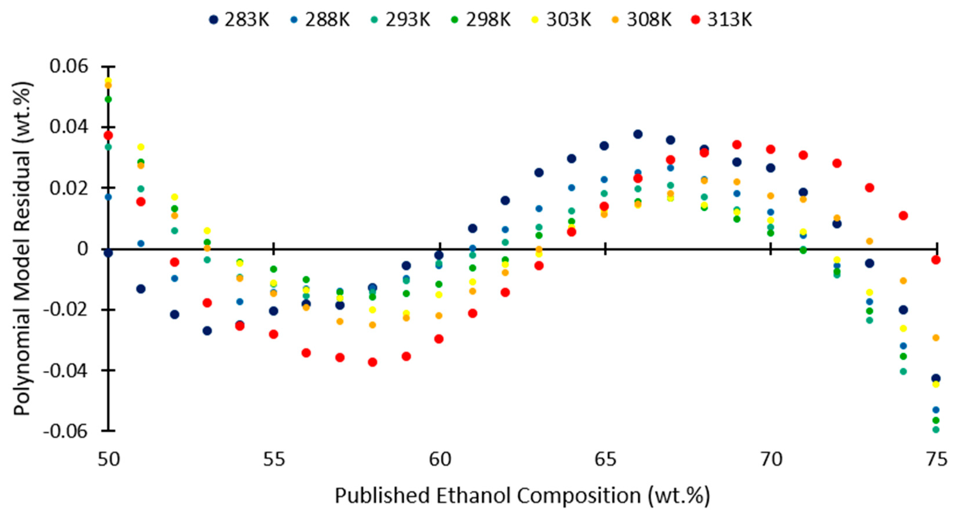
2.2. Polynomial Model

A polynomial correlation was developed to directly compute the composition of ethanol-water solutions from experimental density-temperature measurements, without the use of an iterative solving tool. The optimized polynomial equation uses seven coefficients including a constant, two temperature dependent terms, three density dependent terms, and one cross term which is a function of both temperature and density. The polynomial model is shown in Equation (8) where ( x 2 ) is the mole fraction of ethanol in the binary mixture,   ( ρ ) is the mixture density in ( g c m 3 ) and ( T ) is temperature in Kelvin.
x 2 = θ 1 + θ 2 T + θ 3 ρ + θ 4 ρ 2 + θ 5 ρ 1   + θ 6 T ρ +   θ 7 T 1
The mole fraction composition results computed using Equation (8) can additionally be converted to a mass basis (wt.%) using Equation (9) where ( M W i ) is molecular weight of each component (water (i = 1) and ethanol (i = 2)).
wt . %   ethanol = x 2 M W 2   ( x 2 M W 2 + ( 1 x 2 ) M W 1 ) · 100
An additional advantage of the polynomial correlation is that it can be focused on specific composition ranges to improve the model’s accuracy (e.g., 0–25 wt.% ethanol). The polynomial model coefficients ( θ i ) were regressed over five ethanol-water composition ranges using the same density-composition data set as was used for the R-K model [14]. Table 2 and Table 3 display the polynomial model coefficients and associated errors respectively.

3. Results and Discussion

The Redlich-Kister and polynomial expansion models were evaluated by comparing calculated ethanol-water mixture composition values to literature data reported in Perry’s Handbook [15]. Figure 1 displays a comparison of ethanol composition as a function of density at four temperatures between 283–313 K, where the symbols represent the literature data and the polynomial model results are shown as trend lines. A similar comparison for the Redlich-Kister model is displayed in supplemental information, Figure S1. As shown in Figure 1 and Figure S1, the polynomial expansion and R-K models both accurately computed the composition of ethanol-water mixtures and demonstrated average deviations of 0.37 wt.% and 0.45 wt.%, respectively.
Importantly, while performing the regression analysis we identified two data points in Perry’s Handbook which were incorrectly transcribed from the original source, the International Critical Tables of Numerical Data, Physics Chemistry and Technology [14]. The density values at 25 °C (61 wt.% EtOH) and 40 °C (68 wt.% EtOH) are listed in Perry’s Handbook as 0.88446 g/cm3 and 0.85407 g/cm3 but should be 0.88466 g/cm3 and 0.85507 g/cm3, respectively. We determined that the aforementioned errors moderately impacted the R-K model fit and other researchers using the Perry’s data set should be aware of these two errors. The model coefficients and results generated in this report used the correct density data points as reported in the original reference [14].
The accuracy of each model was further assessed by examining the difference between the computed ethanol composition and the corresponding literature value, herein referred to as the residual. Figure 2 displays the residual plot for the polynomial correlation over an ethanol composition range of 0–100 wt.%. As shown in Figure 2, the largest deviations occur in the 0–20 wt.% ethanol composition range with smaller, non-random, deviations observed between 20–100 wt.% ethanol. Figure 3 displays the residual plot for the Redlich-Kister model where again, the largest deviations were observed in the 0–20 wt.% ethanol composition range.
Comparing Figure 2 and Figure 3 indicates that the R-K model predicts the composition of ethanol-water mixtures at the 0 wt.% and 100 wt.% ethanol endpoints with greater accuracy than the polynomial correlation. This observation can be understood by examining the formulation of the R-K model shown in Equation (3). The Redlich-Kister model computes mixture density as a function of excess molar volume ( V E ) which is directly dependent on composition and is zero for pure components. Therefore, ethanol-water compositions computed by the Redlich-Kister model approach the pure component values at each endpoint where V E = 0 , resulting in the improved accuracy compared to the polynomial model which is not bound at the composition endpoints.
Alternatively, the polynomial correlation is particularly advantageous as it can be optimized for computing mixture composition within specific concentration ranges, resulting in increased accuracy. For example, Figure 4 displays the residual plot for the polynomial model with coefficients fit to data between 50–75 wt.% ethanol. The maximum residuals over this range are much smaller (±0.06 wt.%) compared with the error when the model was trained over the entire 0–100 wt.% composition range (±0.37 wt.%). Table 3 displays the average and maximum residuals for the polynomial model when fit to data in five composition ranges including: 0–25 wt.%, 25–50 wt.%, 50–75 wt.%, 75–100 wt.%, and 0–100 wt.%. The polynomial model can also be optimized by fitting the coefficients to data over a given composition range of interest, providing increased model accuracy for applications where specific ethanol-water mixture compositions are expected.
The residuals displayed in Table 3 demonstrate that the polynomial correlation can compute precise ethanol compositions when modeled using accurate density and temperature inputs. Top of the line Coriolis mass flowmeters measure density and temperature with reported accuracies of ±0.0002 g/cm3 and ±1 K, respectively [16]. These experimental uncertainties result in a computed ethanol composition error of ±0.25 wt.% when calculated using the polynomial correlation. This sensitivity analysis indicates the importance of obtaining accurate experimental density and temperature data when using the correlations presented herein. Furthermore, these correlations are designed for use with binary (1) water + (2) ethanol solutions and the effect of impurities on mixture density and the calculated composition must be carefully examined before applying the methods presented to multicomponent mixtures.

4. Conclusions

The polynomial and Redlich-Kister based correlations developed in this work provide two methods for computing the composition of ethanol-water mixtures for fermentation and chemical processes using experimental temperature and density measurements. The Redlich-Kister model computed ethanol composition with an average deviation of ±0.45 wt.% over the 0–100 wt.% ethanol composition range and required the use of an iterative solving tool. The polynomial model was slightly more accurate (±0.37 wt.% deviation) over this same composition range and permits direct calculation of mixture composition. The polynomial model can also be optimized for specific composition ranges, further increasing the model accuracy. In conclusion, both models presented herein provide methods for accurately calculating on-line ethanol-water composition.

Supplementary Materials

The Figure S1 is available online at https://www.mdpi.com/2311-5637/4/3/72/s1.

Author Contributions

Conceptualization, M.B.S., D.L.M. and B.B.D.; Methodology, M.B.S and D.L.M.; Software, B.B.D.; Validation, B.B.D.; Formal Analysis, B.B.D.; Investigation, B.B.D.; Writing-Original Draft Preparation, B.B.D. and D.L.M.; Writing-Review & Editing, D.L.M. and M.B.S.; Supervision, M.B.S.

Funding

This research received no external funding.

Acknowledgments

The authors thank Andy Shiflett, Kristin Grant, and Rita Lencastre at Novo Nordisk Pharmaceutical Company for the original idea to develop these correlations.

Conflicts of Interest

The authors declare no conflicts of interest.

References

  1. Zion Market Research. Available online: https://www.zionmarketresearch.com/news/fuel-ethanol-market (accessed on 10 March 2018).
  2. Lindsey, B.D.; Ayotte, J.D.; Jurgens, B.C.; Desimone, L.A. Using groundwater age distributions to understand changes in methyl tert-butyl ether (MtBE) concentrations in ambient groundwater, northeastern United States. Sci. Total Environ. 2017, 579, 579–587. [Google Scholar] [CrossRef] [PubMed]
  3. Condon, N.; Klemick, H.; Wolverton, A. Impacts of ethanol policy on corn prices: A review and meta-analysis of recent evidence. Food Policy 2015, 51, 63–73. [Google Scholar] [CrossRef] [Green Version]
  4. Li, H.; Chai, X.S.; Deng, Y.L.; Zhan, H.Y.; Fu, S.Y. Rapid determination of ethanol in fermentation liquor by full evaporation headspace gas chromatography. J. Chromatogr. A 2009, 1216, 169–172. [Google Scholar] [CrossRef] [PubMed]
  5. Weatherly, C.A.; Woods, R.M.; Armstrong, D.W. Rapid Analysis of Ethanol and Water in Commercial Products Using Ionic Liquid Capillary Gas Chromatography with Thermal Conductivity Detection and/or Barrier Discharge Ionization Detection. J. Agric. Food Chem. 2014, 62, 1832–1838. [Google Scholar] [CrossRef] [PubMed]
  6. Buttler, T.A.; Johansson, K.A.J.; Gorton, L.G.O.; Markovarga, G.A. Online Fermentation Process Monitoring of Carbohydrates and Ethanol Using Tangential Flow Filtration and Column Liquid-Chromatography. Anal. Chem. 1993, 65, 2628–2636. [Google Scholar] [CrossRef]
  7. Lidén, H.; Buttler, T.; Jeppsson, H.; Marko-Varga, G.; Volc, J.; Gorton, L. On-line monitoring of monosaccharides and ethanol during a fermentation by microdialysis sampling, liquid chromatography and two amperometric biosensors. Chromatographia 1998, 47, 501–508. [Google Scholar] [CrossRef]
  8. Terol, A.; Paredes, E.; Maestre, S.E.; Prats, S.; Todoli, J.L. Alcohol and metal determination in alcoholic beverages through high-temperature liquid-chromatography coupled to an inductively coupled plasma atomic emission spectrometer. J. Chromatogr. A 2011, 1218, 3439–3446. [Google Scholar] [CrossRef] [PubMed]
  9. Yarita, T.; Nakajima, R.; Otsuka, S.; Ihara, T.; Takatsu, A.; Shibukawa, M. Determination of ethanol in alcoholic beverages by high-performance liquid chromatography-flame ionization detection using pure water as mobile phase. J. Chromatogr. A 2002, 976, 387–391. [Google Scholar] [CrossRef]
  10. Buratti, S.; Ballabio, D.; Giovanelli, G.; Dominguez, C.M.Z.; Moles, A.; Benedetti, S.; Sinelli, N. Monitoring of alcoholic fermentation using near infrared and mid infrared spectroscopies combined with electronic nose and electronic tongue. Anal. Chim. Acta 2011, 697, 67–74. [Google Scholar] [CrossRef] [PubMed]
  11. Mazarevica, G.; Diewok, J.; Baena, J.R.; Rosenberg, E.; Lendl, B. On-line fermentation monitoring by mid-infrared spectroscopy. Appl. Spectrosc. 2004, 58, 804–810. [Google Scholar] [CrossRef] [PubMed]
  12. Veale, E.L.; Irudayaraj, J.; Demirci, A. An on-line approach to monitor ethanol fermentation using FTIR spectroscopy. Biotechnol. Prog. 2007, 23, 494–500. [Google Scholar] [CrossRef] [PubMed]
  13. Zou, X.Y.; Luo, F.; Xie, R.; Zhang, L.P.; Ju, X.J.; Wang, W.; Liu, Z.; Chu, L.Y. Online monitoring of ethanol concentration using a responsive microfluidic membrane device. Anal. Methods-UK 2016, 8, 4028–4036. [Google Scholar] [CrossRef]
  14. National Research Council (U.S.); Washburn, E.W.; West, C.J.; Hull, C. International Critical Tables of Numerical Data, Physics, Chemistry and Technology, 1st ed.; McGraw-Hill book company, Inc.: New York, NY, USA, 1926. [Google Scholar]
  15. Perry, R.H.; Green, D.W. Perry’s Chemical Engineers’ Handbook, 8th ed.; McGraw-Hill: New York, NY, USA, 2008. [Google Scholar]
  16. Micro Motion ELITE Peak Performance Coriolis Flow and Density Meter. Available online: https://www.emerson.com/en-us/catalog/micro-motion-elite-coriolis (accessed on 5 August 2018).
Figure 1. Global comparison of the polynomial model fit to literature density data between 0–100 wt.% ethanol. Data points represent published data and trend lines represent model fit.
Fermentation 04 00072 g001
Figure 2. Weight percent (wt.%) residuals for mixture composition calculated using the polynomial model with coefficients regressed using temperature dependent density data between 0–100 wt.% ethanol.
Fermentation 04 00072 g002
Figure 3. Weight percent (wt.%) residuals for mixture composition calculated using the Redlich-Kister model with coefficients regressed using temperature dependent density data between 0–100 wt.% ethanol.
Fermentation 04 00072 g003
Figure 4. Weight percent (wt.%) residuals for mixture composition calculated using the polynomial expansion model with coefficients regressed using temperature dependent density data between 50–75 wt.% ethanol.
Fermentation 04 00072 g004
Table 1. Optimized coefficients for the R-K model with temperature dependent terms shown in Equations (4)–(6). i = 0 units of cm3∙mol−1, i = 1 units of cm3∙mol−1∙K−1.
Parameteraibici
i = 0−9.054199−4.9307635.286817
i = 10.015720570.01241796−0.01989784
Table 2. Optimized coefficients for the polynomial model shown in Equation (8).
Ethanol Composition Range (wt.%)θ1θ2 (K−1)θ3 (cm3∙g−1)θ4 (cm6∙g−2)θ5 (g∙cm−3)θ6 (cm3∙g−1∙K−1)θ7 (K)
0–100−96.32780−0.0285651298.96611−37.8183835.073420.0284489836.74344
0–251722.515−0.04283923−1786.652612.3505−548.04760.04246920−17.43558
25–50−357.4251−0.01758119381.6007−138.9431114.04150.01808855155.2817
50–75−6.965499−0.02773449−5.9677782.3107378.9934990.03055873255.8742
75–10016.57862−0.03431656−37.5168615.194763.8234820.03827332272.0696
Table 3. Average absolute deviation and largest absolute deviation between ethanol compositions calculated using the polynomial model and published literature data for several composition ranges. Calculations made by using a solving tool to calculate mixture composition using the Redlich-Kister expansion.
Ethanol Composition Range (wt.%)Average Absolute Residual (wt.% Ethanol)
( | p r e d i c t e d l i t e r a t u r e | n )
Largest Residual (wt.% Ethanol)
( m a x | p r e d i c t e d l i t e r a t u r e | )
0–1000.37392.447
0–250.16840.6908
25–500.03070.2435
50–750.017470.05981
75–1000.017770.08352
R-K 0–100 0.45162.682

