POD Analysis of the Wake of Two Tandem Square Cylinders

Abstract

This study aims to investigate the wake of two tandem square cylinders based on the Proper Orthogonal Decomposition (POD) analyses of the PIV and hotwire data. The cylinder centre-to-centre spacing ratio L/w examined is from 1.2 to 4.2, covering the four flow regimes, i.e., extended body, reattachment, transition and co-shedding. The Reynolds number examined was 1.3 × 10⁴. A novel Proper Orthogonal Decomposition (POD) technique (hereafter referred to as POD_HW) is developed to analyse data from single point hotwire measurements, offering a new perspective compared to the conventional POD analysis (POD_PIV) based on Particle Image Velocimetry (PIV) data. A key finding is the identification of two distinct states, reattachment and co-shedding, within the transition flow regime at L/w = 2.8, which POD_PIV fails to capture due to the limited duration of the PIV data obtained. This study confirms, for the first time, the existence of these states as proposed by Zhou et al. (2024), highlighting the advantage of using POD_HW for capturing intermittent flow phenomena. Furthermore, the analysis reveals how the predominant coherent structures contribute to the total fluctuating velocity energy in each individual regime. Other aspects of the flow are also discussed, including the Strouhal numbers, the contribution to the total fluctuating energy of the flow from the first four POD modes, and a comparison between different regimes.

1. Introduction

The study of fluid dynamics around bluff bodies is crucial for various engineering applications, such as bridge piers, high-rise buildings, offshore structures and heat exchanger design [1,2,3,4,5,6]. Square cylinders are of interest due to the way their sharp corners influence the fascinating wake dynamics, including vortex shedding, shear layer, vortex street and recirculation bubble. The flow around a single square cylinder is well-documented, characterized by the formation of a periodic vortex street in its wake [7,8,9,10,11,12,13]. Placing one square cylinder behind another increases the complexity of flow behaviours, via intricate vortex dynamics, increased turbulence, and varying fluid forces on the structures. As such, the wake behind the upstream cylinder significantly impacts the flow around the downstream cylinder, resulting in distinctive flow structures not typically observed around isolated cylinders [1]. Therefore, a comprehensive grasp of the flow topology of two tandem cylinders is vital for accurately predicting forces, shedding frequency and flow-induced vibration [14].

The wake of two tandem cylinders is contingent on Reynolds number (Re), the spacing between the cylinders (L/w), and turbulent intensity, where L is the cylinder centre-to-centre spacing and w is the width of the square cylinder [15,16]. Zhou et al. [1] experimentally studied the dependence of wake topology on L/w and Re, identifying four distinct flow regimes. The extended-body regime (L/w ≤ 1.5–2.0) occurs where two square cylinders behave as a single rectangular cylinder or extended body. In the reattachment regime (1.5–2.0 < L/w < 2.7–3.2), the shear layers separating from the upstream cylinder may reattach to the side surfaces of the downstream cylinder and subsequently separate again from the trailing edges, rolling up periodically. The co-shedding regime (L/w ≥ 3.0–3.4) is characterized by quasi-periodical vortices generated both between and behind the cylinders at the same frequency. Lastly, the transition regime (2.7 ≤ L/w ≤ 3.3) involves a change in the flow structure from reattachment to co-shedding or vice versa, as depicted in Figure 1. Each regime exhibits unique drag and lift characteristics. The study also compared the findings with the wake of two tandem circular cylinders, emphasizing the influence of flow separation points and sharp corners on flow behaviour and classification. Sakamoto et al. [17] at Re = 2.76 × 10⁴ examined flow structure dependence on L/w = 1.5~40 and divided the flow into three regimes: regime I (1.5 ≤ L/w < 4), regime II (4 < L/w < 28) and regime III (L/w > 28). The flows in regimes I and II are respectively characterized by vortex shedding from the downstream cylinder (i.e., reattachment flow) and by vortex shedding from both cylinders with identical Strouhal number. In regime III, two cylinders shed vortices with distinct Strouhal numbers. Shui et al. [18] experimentally studied the flow structures dependence on L/w = 1.5~9.0 and identified six distinct flow regimes: single bluff-body (L/w ≤ 2.5), no vortex shedding (2.5 < L/w ≤ 3.5), shear-layer reattachment (3.5 < L/w ≤ 4.4), synchronization of the vortex shedding (4.4 < L/w ≤ 6.5), two-layered vortices formation (6.5 < L/w ≤ 7.5), secondary vortex formation (7.5 < L/w ≤ 9.0). They also discovered two new modes—the two-layered vortex formation (TVF) and secondary vortices formation (SVF)—and analysed their mechanisms. Liu and Chen [19] conducted an experimental study on the flow around two square cylinders in a tandem arrangement, focusing on the hysteresis of flow transition from reattachment to co-shedding and vice versa when L/w was progressively increased and decreased. The transition from reattachment to co-shedding was delayed with increasing L/w compared to the case of decreasing L/w. Hasebe et al. [20] also reported similar results. Kim et al. [21] studied the flow characteristics around two square cylinders using particle image velocimetry (PIV) for L/w = 1.0~4.0, and Re = 5.3 × 10³ and 1.6 × 10⁴. They found that increasing L/w and Re both cause flow pattern changes from reattachment to co-shedding, leading to discontinuous jumps in the drag coefficient. Yen et al. [22] using PIV captured flow fields for L/w = 1.5–5 and confirmed extended-body, reattachment, and co-shedding flows. Lankadasu and Vengadesan [23] numerically investigated Strouhal numbers of two square cylinders in a planar shear flow. The Strouhal number decreases with increasing shear rate. A sufficiently high shear rate causes the cylinders to shed vortices at multiple Strouhal numbers. The transition L/w from reattachment to co-shedding decreases with increasing shear rate. The downstream cylinder experiences higher fluctuating forces than the upstream cylinder regardless of the shear rate. Numerical methods were also employed by investigators [24,25,26,27,28] to study the effects of the gap between the two square cylinders on the wake.

Proper Orthogonal Decomposition (POD) is a robust statistical technique widely utilized in fluid dynamics to analyse and simplify high-dimensional processes, notably turbulent flows [29,30]. Its effectiveness lies not only in identifying prominent features and phenomena in data but also in compressing extensive datasets to extract underlying physics. By segregating the flow field into orthogonal modes, POD offers an optimal basis set (POD modes) for reconstructing coherent structures. This approach has gained traction, enabling the identification of coherent structures across various flows such as jets, mixing layers, channel flows, isolated cylinder flow, and two-cylinder flow [31,32,33]. POD is useful for studying wake dynamics as it can extract key flow features including spatial and temporal coherence, offering a low-dimensional description of high-dimensional processes. It was first introduced in the study of turbulence by Lumley [34], although it had been independently suggested by several researchers [35,36,37,38,39].

The POD leverages modes extracted from data to discern and prioritize the coherent structures based on energy [30]. In comparison to other identification techniques, POD excels at pinpointing the prominent flow mode in the flow field. Wang et al. [40] explored vortex shedding from square-section building models using PIV and pressure scanning, identifying vortex patterns through POD. They observed antisymmetric modes with single vortices and symmetric modes with counter-rotating vortex pairs. Liu et al. [41] utilized POD to understand the flow structures around a square cylinder near a plane wall. The analysis unravelled a dominant POD mode with vortex shedding from one side of the cylinder and no shedding from the other.

The prior works have extensively delved into the wake dynamics of a single structure using POD. However, the complexity of wake dynamics escalates notably for two tandem cylinders because of the addition of one more dimension L/w, which leads to four distinct flow regimes [1]. Employing POD to capture the dynamic nature of wake for two tandem square cylinders with L/w = 1.4–4.2 and Re = 1.3 × 10⁴, this study aims to investigate the wake of two tandem square cylinders based on the POD analyses of the PIV and hotwire data, thus gaining in-depth insights into the wake dynamics and coherent structures, which are often overlooked in time-averaged flow fields, vortex shedding frequencies, and pressure distributions typically examined in the literature. The focus is given on identifying dominant flow structures, quantifying energy distribution among different modes, and understanding the influence of L/w on wake dynamics. To achieve the objectives, both PIV and hotwire data are analysed using POD. The rationale for using both methods is multifaceted. POD of PIV data provides detailed spatial information on velocity fields, allowing for visualizations of coherent structures, vortex shedding, and near-wake structures. In contrast, POD of hotwire data offers high temporal resolution data at a specific point in the flow, which is crucial for capturing rapid fluctuations and small-scale turbulence that may not be fully resolved in PIV data. Using both techniques allows for cross-validation of results, increasing the robustness and reliability of the findings.

2. Experimental Details & POD Method

2.1. Experimental Setup

Experiments were performed in a closed-circuit wind tunnel, with a test section of 0.6 m × 0.6 m × 2.4 m in height, width, and length, respectively. The floor of the test section was made from a smooth aluminium alloy plate. On the other hand, the side walls and ceiling were made from high-transparency acrylic panels to facilitate laser light transmission and reception for PIV measurements. To minimize the reflection and scattering of laser light, one of the side walls was painted black. The free-stream velocity in the test section ranged from 1.5 to 50 m/s. To measure the free-stream velocity, a Pitot-static tube was linked to a Furness micro-manometer (FCO 510, Furness Controls Ltd., Bexhill, UK). Experiments were conducted at a freestream velocity U_∞ = 10 m/s corresponding to a Re = U_∞w/ν = 1.3 × 10⁴, where ν is the kinematic viscosity of the fluid. The uncertainty in U_∞ was measured to be around ±1.0% of the average value and the free-stream turbulence intensity T_u was estimated to be 0.13% in the absence of cylinders.

Two identical square cylinders made of aluminium alloy were positioned in the horizontal mid-plane of the test section (Figure 2). The cylinders arranged in tandem extended across the entire height of the test section, resulting in a maximum blockage ratio of 3.18%. Each square cylinder had a side width of w = 19.1 mm and a span length of L = 605 mm, resulting in an aspect ratio (L/w) of 31.6. Given the relatively small blockage ratio, based on the findings of West & Apelt (1982) [42], no corrections to the measurements were deemed necessary. Moreover, due to the sufficiently large aspect ratio, the end effects of the rectangular cylinders can be considered negligible. Two Cartesian coordinate systems, (x-O-y) and (x′-O′-y′), are defined with the origin at the centres of the two cylinders (Figure 2). The x-or x′-axis aligns with the freestream velocity while the y-or y′-axis represents the cross-stream direction. The y-or y′-axis represents the span of the upstream and downstream cylinders, respectively.

2.2. Hotwire Measurements

One single-component hotwire anemometer, calibrated using a Pitot tube and a highly precise electronic pressure transducer, was used to measure the fluctuating streamwise velocities u in the wake of the downstream cylinder (Figure 1). The hotwire probe (55P01, DANTEC Dynamics, Skovlunde, Denmark) was placed at x′* (=x′/w) = 1.0, and y′* (=y′/w) = −1.5 to determine the vortex shedding characteristics in the wake of the downstream cylinder, as shown in Figure 2. The probe was meticulously positioned at the locations where the fluctuating signals reached their approximate maximum. The sensing element of the hotwire was made of tungsten wire with a diameter of 0.5 µm and a length of 1.25 mm. The hotwire was operated at an over-heat ratio of 1.5 using a constant-temperature anemometer (Dantec Streamline, DANTEC Dynamics, Skovlunde, Denmark). The hotwire output signals from the anemometer are routed through buck and gain circuits and then low-pass filtered with a cut-off frequency of 1 kHz. The signal is then digitized using a 16-channel A/D board (NI PCI-6143, National Instruments, Austin, Texas, United States) at a sampling frequency f_samp of 2 kHz and recorded on a personal computer for a duration of 60 s for each L/w examined. The hotwire was not calibrated because the measured u value is only used for POD analysis where the fluctuating component of u is required.

2.3. PIV Measurements

A Dantec high-speed PIV system was utilized to capture the flow in the near wake of the cylinders in the (x, y) plane at the midspan z = 0. The flow was seeded with smoke particles approximately 1 μm in diameter, which was produced from paraffin oil using a TSI 9307-6 particle generator. The Stokes number was calculated to be 0.016 within the experimental range [43,44], which is significantly smaller than one, allowing the particles to quickly adjust to the flow. Flow illumination was achieved using two pulsed laser (Litron LDY304-PIV, Nd:YLF) sources emitting at a wavelength of 527 nm, each capable of delivering a maximum power of 30 mJ per pulse. A cylindrical optical lens was affixed to the laser head’s exit to expand the laser beam into a laser light sheet approximately 1 mm thick. The interval between successive pulses was 75 μs, during which a particle could travel only 0.75 mm (5 pixels) at U_∞ = 10 m/s [45]. A high-speed digital CCD camera (Phantom V641, double frames, with a resolution of 2560 × 1600 pixels) was employed to capture particle images using a 50 mm fixed-focus lens. They were recorded at a frame rate of 1000 frames per second (fps) with an exposure time of 1 s. The pixel array of the CCD camera was mapped to a physical region of 384 mm × 240 mm corresponding to a spatial resolution of 0.15 mm/pixel. The magnification factor for the camera setup is approximately 150. The size of the interrogation window was set to 32 × 32 pixels with a 50% overlap in both x and y directions to enhance the resolution and precision of the velocity vector fields. The experimental uncertainty associated with velocity determinations using our current PIV system is estimated to be less than 2%. The particle density N_I—the mean number of particles within an interrogation region—was greater than 10 [46]. A total of 1000 images was captured to calculate both instantaneous and time-averaged velocity fields, including velocity-vector-based POD, vorticity contours-based POD, and sectional streamline patterns, in the (x, y) plane for each L/w examined. Furthermore, the processing of PIV data in our study was conducted using DynamicStudio 6.9 software by DANTEC Dynamics. This software features built-in capabilities for image pre-processing before vector acquisition, including an automatic calibration function designed to remove background noise. An error-checking and interpolation approach was used to identify and correct spurious vectors. In most cases, less than 1% of spurious vectors were detected on instantaneous fields. These outliers were then replaced with interpolated values to maintain the integrity of the velocity fields.

2.4. POD Analysis of PIV Data

The snapshot POD method, initially introduced by Sirovich [29], is utilized to analyse the PIV data. This method is particularly advantageous when the spatial data size is considerably larger than the number of available images, which is often the case in PIV measurements. In this approach, each instantaneous PIV dataset is viewed as a snapshot of the flow field, allowing for the application of the POD technique to extract dominant flow structures and characteristics. Previous studies have successfully employed the POD technique on PIV data [47,48,49,50,51]. This methodology enables a detailed analysis of flow dynamics, coherent structures, and energy distribution within the flow field, providing valuable insights into the wake dynamics behind two tandem square cylinders.

The first step is to determine the mean velocity field (zero mode of POD). The mean velocity field is then subtracted from each instantaneous snapshot. This ensures POD modes based on the fluctuating components (uⁿ_i, vⁿ_i) of the velocity, where u and v represent the fluctuating velocities in the streamwise and lateral directions, respectively. The index n iterates through the N snapshots, while the index i iterates through the M positions of the velocity vectors in each snapshot.

All fluctuating velocity components from N snapshots are organized into a matrix U, as follows:

$$\begin{array}{c}U={[u}^1,u^2\dots u^N]\left[\begin{array}{cccc}{u}_1^1& u_1^2& \dots & u_1^N\\ ⋮& ⋮& ⋮& ⋮\\ u_M^1& u_M^2& \dots & u_M^N\\ v_1^1& v_1^2& \dots & v_1^N\\ ⋮& ⋮& ⋮& ⋮\\ v_M^1& v_M^1& \dots & v_M^1\end{array}\right]\end{array},$$

(1)

The autocovariance matrix C is formed:

$$C=U^{T}U,$$

(2)

A set of N eigenvalues λⁱ and the corresponding set of eigenvectors Aⁱ satisfy

$$C{A}^i={\lambda }^i{A}^i,$$

(3)

The eigenvalues are ordered in descending order as λ¹ >λ² >…> λ^N > 0. Each eigenvalue represents the energy contained by its corresponding mode. The normalized POD modes φⁱ are constructed from the projection of the eigenvectors Aⁱ as follows:

$${\phi }^i={\displaystyle \frac{\sum _1^N{A}_n^i{u}^n}{∥\sum _1^N{A}_n^i{u}^n∥}}, i=\mathrm{1,2},\dots N,$$

(4)

The discrete 2-norm is defined as the following:

$${\parallel \eta \parallel }^2=\sqrt{{\eta }_1^2+{\eta }_2^2+\cdots +{\eta }_M^2},$$

(5)

Each snapshot can be expanded in a series of POD modes with expansion coefficients aⁱ for each φⁱ. The coefficients aⁱ, also called POD coefficients, are determined by projecting the fluctuating part of the velocity field in POD modes:

$$a^n={\Psi }^T{u}^n,$$

(6)

where Ψ = [φ¹, φ², …φ^N]. Then, the expansion of the fluctuation part of a snapshot n is obtained from

$$u^n={\sum }_{i=1}^N{a}_i^n{\phi }^i,$$

(7)

For further details on the POD method, readers can consult Sirovich [29]. Its effectiveness and suitability for time-resolved PIV data have been well-documented by Meyer et al., Kikitsu et al., and Kawai et al. [48,50,51]. In the following discussions, the POD coefficients aⁱ are normalized by their corresponding eigenvalues λⁱ:

$$a_i^{\mathrm{*}}={\displaystyle \frac{a_i}{\sqrt{2{\lambda }^i}}},$$

(8)

To examine the effects of varying the number of snapshots on POD outcomes, PIV data analyses were conducted using datasets of 500, 800, and 1000 snapshots. The POD modes and accompanying coefficients showed remarkable consistency across these datasets, with minor random fluctuations observed only in the higher modes, which are beyond the focus of this study. A total of 1000 images were captured to calculate both instantaneous and time-averaged velocity fields, including velocity-vector-based POD, vorticity contours-based POD, and sectional streamline patterns in the (x, y) plane for each L/w examined. Consequently, the POD analysis can provide up to 1000 modes. The results are however presented for the first five modes, given that higher-order modes have negligible energy.

2.5. POD Analysis of Hotwire Data

Hotwire anemometry, with its high-frequency response and fine spatial resolution, captures time-resolved velocity data at specific points, which is then organized into a snapshot matrix. However, single-point hotwire data present a challenge in creating a comprehensive velocity correlation matrix U^TU due to insufficient flow field information. To overcome this, the signals from a single hotwire are arranged into a trajectory matrix using a method of delays, as described by Broomhead & King [52].

The original signals (u(t) = u(t₁), u(t₂), u(t₃), … u(t_N), u(t_N+1) …,) (where t_N is the Nth data point) measured by a single point hotwire are arranged as follows:

$$U=\left[\begin{array}{cccc}u\left(t_1\right)& u\left(t_2\right)& \cdots & u\left(t_K\right)\\ u\left(t_2\right)& u\left(t_3\right)& \cdots & u\left(t_{K+1}\right)\\ u\left(t_3\right)& u\left(t_4\right)& \cdots & u\left(t_{K+2}\right)\\ ⋮& ⋮& \cdots & ⋮\\ u\left(t_{N-1}\right)& u\left(t_N\right)& \cdots & u\left(t_{N+K-2}\right)\\ u\left(t_N\right)& u\left(t_{N+1}\right)& \cdots & u\left(t_{N+K-1}\right)\end{array}\right],$$

(9)

The matrix is referred to as the trajectory matrix, where N indicates the number of rows and K is the number of columns corresponding to the embedding dimension.

The velocity correlation matrix is given by

$$R_{ij}\left(x,x+r\right)=\sum _{p=1}^N{U}_{pi}^T{U}_{pj}=\sum _{p=1}^{N}u\left(t_{p+i-1}\right)u\left(t_{p+j-1}\right),$$

(10)

After determining the eigenvalues and eigenvectors of Equation (5), the state spaces can be reconstructed by projecting the trajectory matrix U onto the eigenvectors in the dynamical systems analysis. This method is commonly used to create state spaces from single-point data in the analysis of several dynamical systems [52]. In this study, we use the method of Broomhead & King [52] to analyse experimental data from a single hotwire. The resulting matrix U has the following features:

• The rms values of the K columns in U are nearly equal.
• N is significantly larger than K (N >> K).
• Each column statistically contains the same information across all turbulent scales, meaning the velocity spectra of all columns collapse.
• The velocity correlation matrix is given by Equation (10).

After the formation of the velocity correlation matrix, the rest of the POD analysis is identical to the POD analysis of PIV data. The POD analysis of hotwire data was conducted with K = 500 and 1000 (N = 65,000) to examine the impact of the number of columns (K) and rows (N) in Equation (9). The energy distributions and coefficients for the first two modes are nearly identical for these two sets of data, as are the results for N = 65,000 and 130,000 (K = 1000). Therefore, K ≥ 500 and N ≥ 65,000 are sufficient for reasonable accuracy in the current POD analysis of hotwire data. The values N = 65,000 and K = 1000 are therefore generally used for the results presented below.

3. Results and Discussions

Experimental data analysis primarily aimed to identify and characterize the dominant flow structures, coherent patterns, and vortex-shedding frequencies in the wake behind two tandem square cylinders. These structures were identified using various methods with different levels of precision and complexity. We obtained snapshot POD modes, mode energy distribution, and power spectra of dominant POD modes in the wake of the cylinders for L/w = 1.4, 2.4, 2.8 and 4.2.

3.1. POD Modes and Energy Distribution

As explained in Section 2.4, the eigenvalue λⁱ denotes the percentage contribution of the relevant POD mode to the total turbulent kinetic energy (TKE) or turbulent fluctuation energy. The energy distribution to the total fluctuation energy contributed from different POD modes is illustrated in Figure 3. Here, the results in Figure 3a,b and Figure 3c,d are respectively from POD analysis of PIV data (POD_PIV) and hotwire data (POD_HW) at x/w = 1.5, y/w = 1.5. The results of van Oudheusden et al. [31] for a two-dimensional cylinder wake at Re = 1 × 10⁴ are also provided for comparison. The energy contribution markedly decreases as the POD mode number increases for all L/w values and single cylinder wake in the cases of both POD_PIV and POD_HW.

Single cylinder: For a single square cylinder wake as reported by van Oudheusden et al. [31], the first two modes make a substantially larger contribution to the total energy content or TKE than the other modes, and this contribution is greater than that observed in the two tandem square cylinders wake (Figure 3a,b). The results indicate that the first two modes account for approximately 75.2% of the total energy content while modes 3–5 collectively represent only about 5.86%.

Extended-body regime (L/w = 1.4): The first two modes contribute more to the total energy than the other modes, accounting for 31.25% and 26.7%, respectively, and totalling over 58% of the total energy (Figure 3a,b). On the other hand, modes 3–5 together only amount to about 7.28%. Therefore, the wake is dominated by the first two modes linked to the formation of large-scale coherent structures resulting from vortex shedding (Figure 4a). The cumulative mode energy is significantly smaller in the extended-body regime than in the single-cylinder case (Figure 3b).

Reattachment regime (L/w = 2.4): As the regime progresses from the extended-body regime to the reattachment regime (i.e., L/w = 1.2 to 2.4), the contributions of the first two modes decrease slightly to 28.66% and 25.83%, respectively, totalling about 55% of the total energy. On the other hand, modes 3–5 collectively account for approximately 6.28%. This suggests that the dominance of the first two modes diminishes in the reattachment. Yet, the first two modes display large-scale coherent flow structures in the near wake (Figure 5a). The cumulative mode energy is lower in the reattachment regime than in the extended-body regime (Figure 3b).

Transition regime (L/w = 2.8): In the transition regime, the contributions of the first two modes decrease even further to 20.4% and 17.8%, respectively, totalling 38.2%, while modes 3–5 contribute only about 3.9%. The first two modes are thus weak compared to those in the extended and reattachment regimes. The cumulative mode energy in the transition regime is notably lower compared to the extended-body and reattachment regimes (Figure 3b). This decline can be attributed to the reduced coherence of the dominant vortex-shedding process in this transitional regime (Figure 6).

Co-shedding regime (L/w = 4.2): Here, modes 1 and 2 contribute 21.8% and 20.7%, respectively, amounting to a combined total of 42.5%, while modes 3–5 collectively represent 8.83% of the total. This shows a 4% increase in the total energy of the first two modes compared to the transition regime. Yet, the total energy of the first two modes is smaller in the co-shedding flow than in the extended-body or reattachment flow because vortices become smaller in size and strength in the former flow than in the latter (Figure 7a).

Table 1. Comparison of Energy distribution in POD analysis for POD_PIV between the present and single cylinder data. L/w: cylinder spacing ratio.

	L/w = 1.4	L/w = 2.4	L/w = 2.8	L/w = 4.2	Single Cylinder
Mode 1	31.25%	28.66%	20.4%	21.8%	42.6%
Mode 2	26.7%	25.83%	17.8%	20.7%	32.6%
Mode 3	2.25%	2.30%	1.4%	3.68%	2.6%
Mode 4	1.97%	1.76%	1.3%	2.60%	2.2%
Mode 5	1.63%	1.19%	1.2%	2.55%	1.06%

presents the relative energy contributions of the first five POD_PIV modes at different L/w regimes. The first two modes contribute about 55% of the energy in the extended and reattachment regimes while their contribution drops to about 42% in the co-shedding regime. The transition regime has the lowest contribution, about 38%.

In Figure 3c,d, the first two modes of the POD_HW contribute approximately 72.5% of the total energy for a single cylinder [31]. The observation is consistent with the first two POD_PIV modes. For tandem cylinders, the first two modes contribute around 62%, 48%, 44%, and 45% for L/w = 1.4, 2.4, 2.8, and 4.2, respectively. POD_HW extracts the information from a single-point in the hotwire data, that is, this information is from a single point in the flow field. On the other hand, POD_PIV extracts the information from the entire flow field captured by the PIV data. As such, the information extracted is a spatial average of the flow field. The former is a new data analysis technique proposed in this work and has several advantages over the latter. Firstly, the required data can be from a single point. This is crucial in some cases. For example, using a hotwire-based probe to capture the three components of the vorticity vector in a turbulent flow (Zhou et al., 2003 [53], Chen et al., 2016 [54]), which involves four X-wires and is highly challenging even for single-point measurements. It would be extremely challenging to use such probes to measure simultaneously more than two points in the flow field. Secondly, the sampling frequency and duration of the single-point measurement can easily be made adequately large so as to capture some special physical phenomenon. For instance, the present hotwire data sampling (also in Zhou et al., 2024 [1]) lasted for more than one hour at a sampling frequency of 2000 Hz, successfully capturing both reattachment and co-shedding states in the transition regime. In contrast, it would be almost impractical to take continuous PIV images at such a high frequency and lengthy duration in most laboratories. As such, our PIV data failed to capture the two states in the transition regime. The results from POD_HW bear some similarity to those from POD_PIV to some extent, and some discrepancies as expected, given that hotwire results are from a single point measurement. The results from hotwire data are expected to be dependent on the measurement point as the coherent structures weaken with x/w. Yet, credit can be attributed to the hotwire data for producing qualitatively similar trends.

3.2. Wake Characteristics

We focus on the first four POD_PIV modes here as mode 5 and higher modes contribute minimally to the total energy. Figure 4, Figure 5, Figure 6 and Figure 7 present the u contours, velocity vectors, and corresponding streamline patterns for the first four modes. In the u contours (Figure 4, Figure 5, Figure 6 and Figure 7(a₁–a₄)), the structures of modes 1 and 2, as well as modes 3 and 4, appear in pairs. Specifically, the contour structures of modes 1 and 2 at L/w = 1.4–4.2 are highly correlated, indicating alternating vortex shedding [55]. Mode 2 can be understood as a streamwise shift of mode 1, with a phase lag of approximately 1/4 of the shedding circle. In mode 1, a pair of opposite-signed structures form immediately behind the cylinder, while in mode 2, that pair shifts downstream, and a new pair issues from the cylinder. Modes 1 and 2 at L/w = 4.2 (Figure 7(a₁,a₂)) exhibit small-scale vortex structures compared with those at smaller L/w = 1.4–2.8 (Figure 4, Figure 5 and Figure 6(a₁,a₂)). Modes 3 and 4 show smaller-scale vortex structures for L/w = 1.4–2.8 (Figure 4, Figure 5 and Figure 6(a₃,a₄)) but large-scale structures for L/w = 4.2 (Figure 7(a₃,a₄)), reflecting higher flow complexity.

The velocity vector fields (Figure 4, Figure 5, Figure 6 and Figure 7(b₁–b₄)) visually demonstrate the presence of large-scale vortical structures in the first two modes, which align with the modes that contain the highest energy, as confirmed by the mode energy analysis presented in Figure 3. This correspondence between the vector plots and the mode energy distribution implies that the first two modes contain most of the kinetic energy in the flow fields.

Streamline patterns display distinct patterns in the vortex structures (Figure 4, Figure 5, Figure 6 and Figure 7(c₁–c₄)). At L/w = 1.4, 2.4, and 2.8, modes 1 and 2 have two and three vortices, respectively, on the wake centreline in the measurement domain. Indeed, one pair of structures in the u contours represents one vortex in the streamline pattern. Specifically, at L/w = 1.4, mode 3 comprises two symmetric vortices while mode 4 has three pairs of symmetric vortices. At L/w = 2.4, modes 3 and 4 exhibit three and four pairs of symmetric vortices, respectively. At L/w = 2.8, modes 3 and 4 both feature three pairs of vortices. At L/w = 4.2, mode 1 displays the formation of a single vortex followed by two pairs of vortices, whereas mode 2 shows two pairs of vortices. Mode 3 displays no vortices, whereas mode 4 exhibits two symmetric vortices on the wake centreline. These results indicate that the co-shedding flow is more complex in view of flow modes than the extended-body and reattachment flows.

3.3. Identification of Flow Configurations Using POD_PIV Coefficients

Given the limited energy contribution from mode 3 and higher, the phase-resolved component of the flow can be approximated using a low-order flow model that incorporates only the first two POD modes as shown in Equation (11). Van Oudheusden et al. [31] suggested an empirical method (Equation (12)) to determine the phase-resolved component for each snapshot.

$${\overrightarrow{u}}_{LOM}\left(\overrightarrow{x},\phi \right)=\overrightarrow{U}\left(\overrightarrow{x}\right)+a_1\left(\phi \right)\cdot {\overrightarrow{\varphi }}_1\left(\overrightarrow{x}\right)+a_2\left(\phi \right)\cdot {\overrightarrow{\varphi }}_2\left(\overrightarrow{x}\right),$$

(11)

$$a_1=\sqrt{2{\lambda }_1}\mathit{sin}\left(\phi \right)a_2=\sqrt{2{\lambda }_2}\mathit{cos}\left(\phi \right),$$

(12)

where u_LOM is the reconstructed instantaneous velocity field and φ is the vortex-shedding phase angle [56]. The low-order model omits higher-order modes including higher-order harmonics of the coherent motion and random turbulent fluctuations. The first pair of modes truly represents the orthogonal components of the fundamental coherent structures. The verification can be achieved by cross-plotting the mode coefficients a₁ and a₂ from individual realizations. As indicated in the equation, these coefficients, while statistically uncorrelated, are not independent. Instead, they are expected to form an elliptical pattern in the (a₁, a₂) plane:

$${\displaystyle \frac{a_1^2}{2{\lambda }_1}}+{\displaystyle \frac{a_2^2}{2{\lambda }_2}}=1,$$

(13)

This application of POD in the current study involves the direct phase identification of individual flow field realizations. Projecting a specific realization onto the POD modes, we can obtain mode coefficients a₁(i) and a₂(i). The phase φⁱ is then determined as the angle in the normalized (a₁, a₂) plane, given by:

$${\displaystyle \frac{a_1\left(i\right)}{\sqrt{2{\lambda }_1}}}=r_i\mathit{sin}\left({\phi }_i\right){\displaystyle \frac{a_2\left(i\right)}{\sqrt{2{\lambda }_2}}}=r_i\mathit{cos}\left({\phi }_i\right),$$

(14)

where r_i represents the “radius” of the normalized ellipse passing through a₁(i) and a₂(i):

$$r_i^2={\displaystyle \frac{a_1(i{)}^2}{2{\lambda }_1}}+{\displaystyle \frac{a_2(i{)}^2}{2{\lambda }_2}},$$

(15)

Once the phase of each realization is identified, the data ensemble can be sorted by phase to produce phase-resolved or phase-averaged representations of the vortex-shedding cycle.

Figure 8 validates this relationship, displaying a circle in the normalized a₁-a₂ plane. At L/w = 1.4, the cross-plot of normalized a₁ and a₂ forms an approximate circle, confirming the relationship shown in Equations (11) and (12). The ideal circle (solid line) shown in Figure 8a is r = 1. Naturally, all data are not on the line because of cycle-to-cycle variations in the vortex-shedding process [31]. The data points near the origin indicate limited energy contributions from the first two modes due to the small absolute values of a₁ and a₂, with the instantaneous flow field dominated by mode 3 or higher.

As L/w increases to 2.4 (Figure 8b), more data points appear close to the circle, with almost no data near the circle centre. That is, alternate reattachment of the shear layers enhances orthogonality in the vortex shedding. The same observation is made for L/w = 4.2 where no data appear near the centre (Figure 8d). Here, the gap vortex impingement triggers vortex shedding from the downstream cylinder [57,58] and enhances orthogonality in the vortex shedding. On the other hand, at L/w = 2.8, the data disperse from the circle, with more data points lying close to the circle centre as the switch of flow from reattachment to co-shedding and vice versa deteriorates the orthogonality (Figure 8c).

Figure 9 shows temporal variations and power spectra of the POD coefficients of the first four dominant modes at L/w = 1.4, 2.4, 2.8, and 4.2. With a phase shift of π/4, modes 1 and 2 are periodic, linked with alternate vortex shedding. The alternation between negative and positive values represents the formation of clockwise and counterclockwise vortices. In contrast, modes 3 and 4 display random or relatively chaotic behaviour, which indicates turbulent characteristics.

The power spectra presented in Figure 9 were obtained using a fast Fourier transform (FFT) of POD coefficients, with a window size (N_w) of 4096, providing a frequency resolution Δƒ (=f_samp/N_w) of 0.49 Hz in the spectral analysis [59]. The Strouhal number St = fw/U_∞, where f is the shedding frequency. The power spectra of the first and second modes display a prominent peak at the Strouhal number St = 0.12~0.14, corresponding to the vortex-shedding frequency of the upstream and downstream cylinders. These findings are consistent with previous results reported by Zhou et al. [1]. At L/w = 1.4, the spectrum of mode 4 displays a peak at St = 0.28, which is twice the St of modes 1 and 2. Similarly, modes 3 and 4 also show a peak each at St = 0.26 for L/w = 2.4 and 2.8, which is again double the St of modes 1 and 2 (Figure 9b,c). The peak amplitude at L/w = 2.4 is significantly larger than that at L/w = 1.4. The peak amplitudes associated with modes 1 and 2 (St = 0.12) decline when L/w increases from 2.4 to 2.8, as do those with modes 3 and 4. At L/w = 4.2, the peak amplitudes for modes 1 and 2 heighten and then return to a level comparable to those at L/w = 1.4 and 2.4. Unlike other L/w values, mode 4 at L/w = 4.2 displays a wideband peak at St = 0.12 corresponding to the St of modes 1 and 2.

3.4. Further Analysis of Transition Flow

Figure 10 presents the time histories of the hotwire-measured u for the transition regime (L/w = 2.8). The hotwire signal reveals that the transition regime exhibits two distinct states: reattachment and co-shedding, characterised by low- and high-amplitude u, respectively, as detailed in Zhou et al. [1]. The PIV however fails to capture this flow feature. The hotwire signal shows that the switch from reattachment to co-shedding, and vice versa, is intermittent, with intervals on the order of 10 s or more. Figure 11 shows typical temporal variations and power spectra of the POD_HW coefficients of the first four dominant modes for L/w = 2.8. These modes demonstrate that the transition involves a change in the flow field from reattachment to co-shedding, or vice versa. The co-shedding and reattachment flows correspond to St = 0.10 and 0.13, respectively, characterized by large- and small-amplitude fluctuations. The peak at the latter St is thus less pronounced than that at the former. These findings are consistent with prior results reported by Zhou et al. [1]. The reattachment and co-shedding flow states coexist in POD_HW modes 1–4, as reflected in Figure 11 as well. This flow feature is not captured by POD_PIV analysis.

4. Conclusions

The wake of two tandem square cylinders is investigated based on the POD_HW and POD_PIV analyses of hotwire and PIV data, measured at Re = 1.3 × 10⁴ and L/w = 1.4–4.2, covering all four regimes of this flow. While the conventional POD_PIV works on the PIV data from a flow field, the POD_HW may be used to analyse the data from a single point hot-wire. The following conclusions can be drawn from this investigation:

• A POD technique POD_HW has been developed for the analysis of single-point hotwire data. The traditional POD method is usually performed on data obtained either from PIV measurements or hotwire array or direct numerical simulations data where the two-point space-correlation tensor should include information at two different space points at least. However, POD_HW may be applied for the analysis of single-point hotwire measurements, which are characterized by high-frequency response and fine spatial resolution. More importantly, this method can be used for all other data from a single point such as the single-point 3-D vorticity data, obtained from an 8-wire vorticity probe [60,61], where it would be highly challenging to simultaneously measure vorticity at two points.
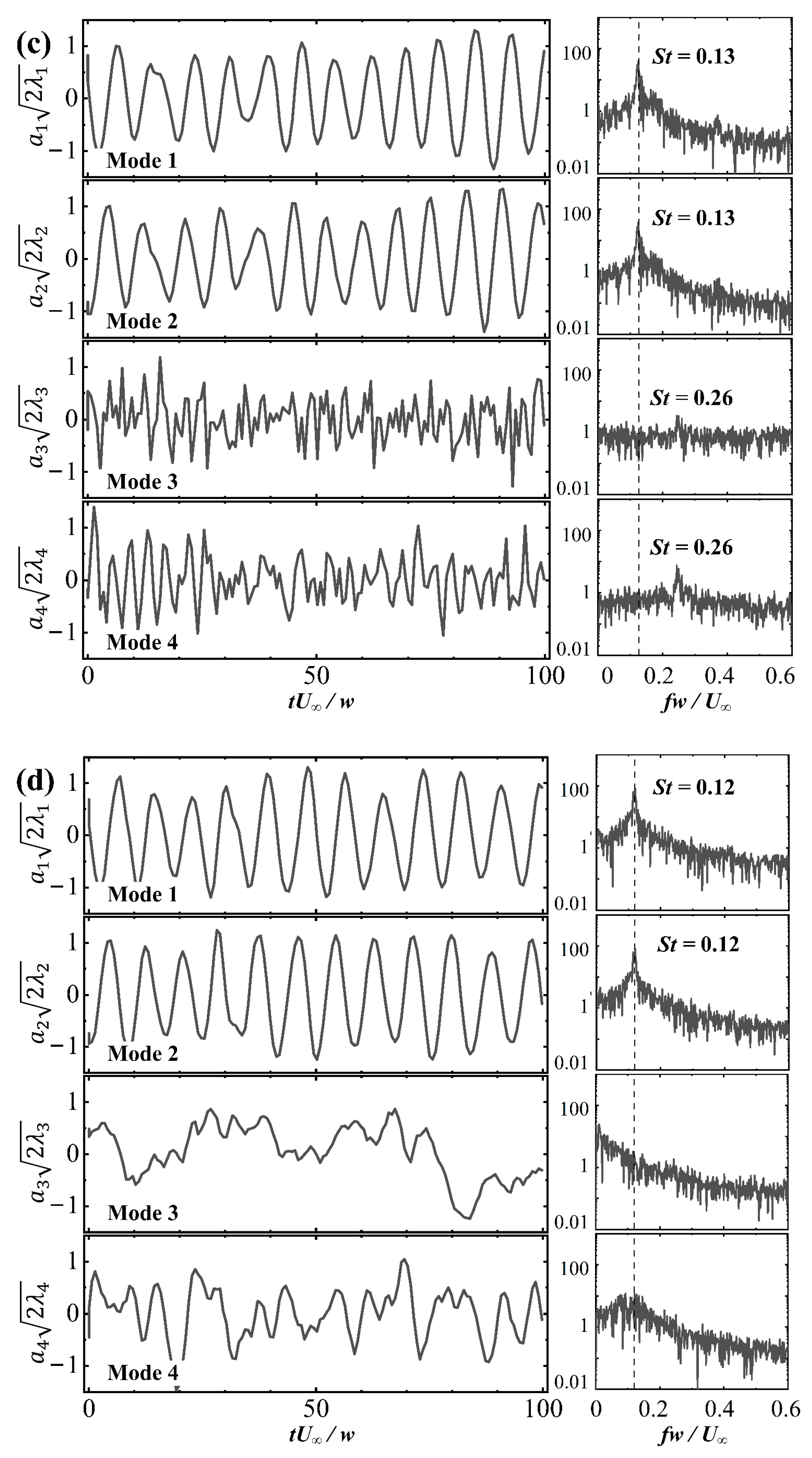
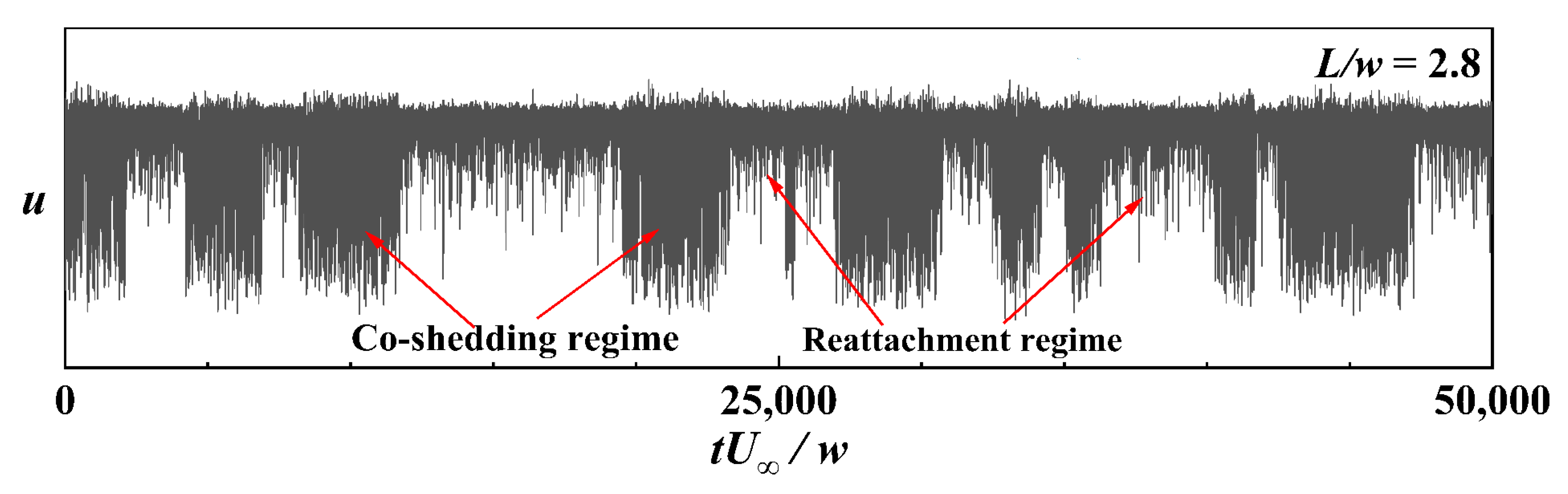
• It has been found from the data analysis using POD_HW that the transition flow regime (L/w = 2.8) is characterized by two distinct states, i.e., reattachment and co-shedding, characterized by St = 0.13 and 0.10, respectively, thus confirming convincingly for the first time the proposition by Zhou et al. (2024) [1]. On the other hand, POD_PIV fails to capture this flow feature. As shown from the hotwire signal, the switch from reattachment to co-shedding or vice versa in the transition regime is intermittent, the interval being in the order of 10 or dozens of seconds. As such, this physical phenomenon can be captured by the hotwire data with a duration of 10 min but missed by the high-speed PIV data (about 1000 images) in the duration of a couple of seconds, which explains the different results between POD_HW and POD_PIV analyses.
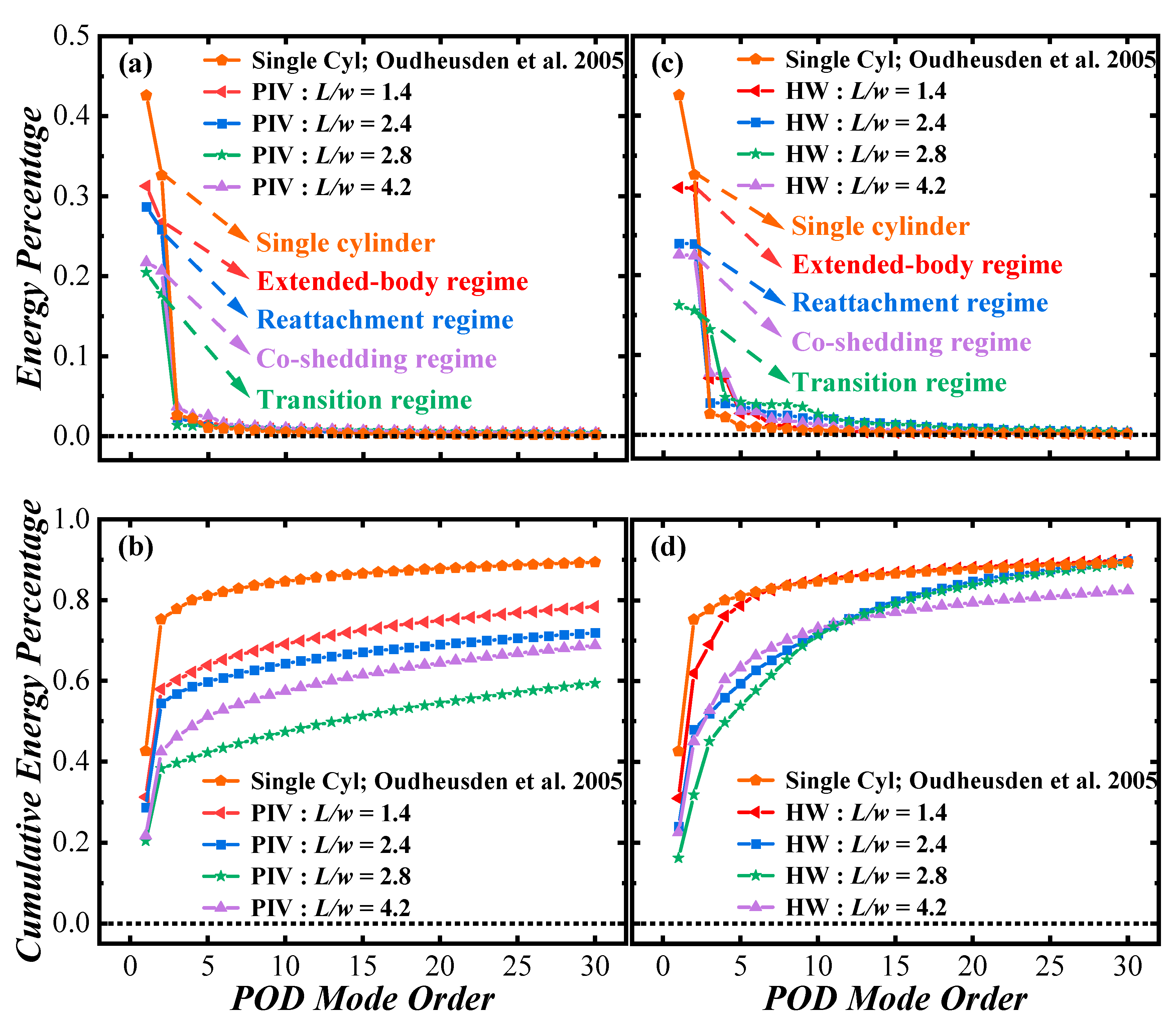
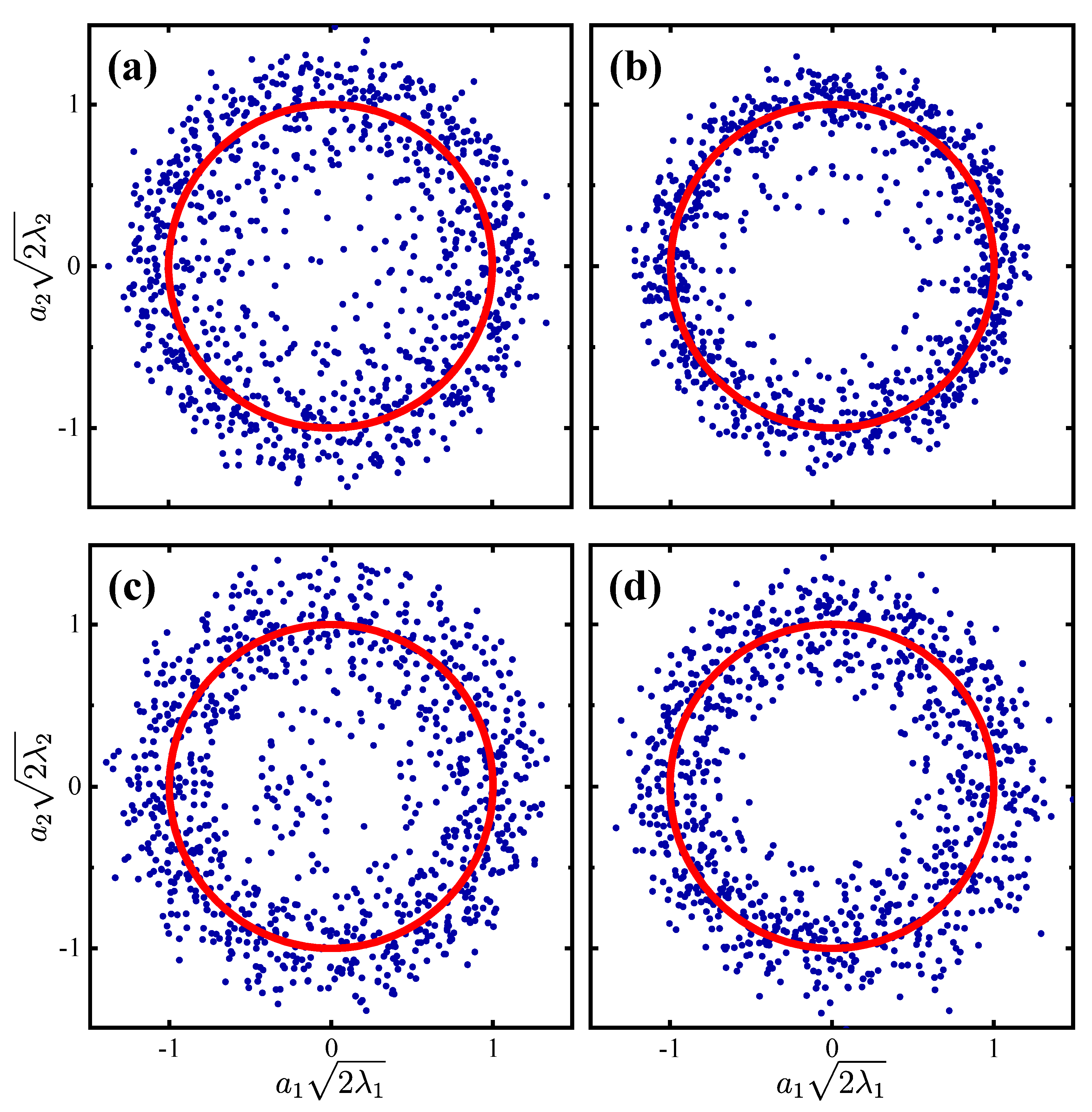
• The contribution from the predominant coherent structures to the total fluctuating velocity energy is documented for different regimes. The first two POD_PIV modes contribute 58.0%, 54.5%, and 42.5% to the total fluctuating energy in the extended-body, reattachment, and co-shedding regimes, respectively. The two modes are highly correlated, exhibiting alternating vortex-shedding patterns, irrespective of L/w, apparently representing the Karman vortex streets, while the higher-order modes (3 and beyond) exhibited more random and chaotic behaviour. Since the POD_PIV fails to capture both co-shedding and reattachment states, we have to rely on POD_HW to determine the contribution from the predominant coherent structures to the total fluctuating velocity energy. The transition regime behaves differently from the other three regimes. The first, second and third POD_HW modes make significant contributions to the total fluctuating velocity energy, accounting for 16.2%, 15.6%, and 13.2%, respectively (with the contribution of 4.7% from the fourth mode), due to the presence of both co-shedding and reattachment states. The Karman vortex strength in the transition regime (L/w = 2.8) is weakest of all, as indicated by the least pronounced peak at St in the power spectra of the first two POD_PIV modes.

References

1. Zhou, Y.; Hao, J.; Alam, M.M. Wake of Two Tandem Square Cylinders. J. Fluid Mech. 2024, 983, A3. [Google Scholar] [CrossRef]
2. Heidari, M. Wake Characteristics of Single and Tandem Emergent Cylinders in Shallow Open Channel Flow. Doctoral Dissertation, University of Windsor, Windsor, ON, Canada, 2016. [Google Scholar]
3. Marble, E.; Morton, C.; Yarusevych, S. Pod Analysis of the Wake Development of a Pivoted Circular Cylinder Undergoing Vortex Induced Vibrations. Presented at the Fluids Engineering Division Summer Meeting 2017, Waikoloa, HI, USA, 30 July–3 August 2017. [Google Scholar]
4. Alam, M.M.; Zhou, Y.; Wang, X. The Wake of Two Side-by-Side Square Cylinders. J. Fluid Mech. 2011, 669, 432–471. [Google Scholar] [CrossRef]
5. Higham, J.; Brevis, W. Modification of the Modal Characteristics of a Square Cylinder Wake Obstructed by a Multi-Scale Array of Obstacles. Exp. Therm. Fluid Sci. 2018, 90, 212–219. [Google Scholar] [CrossRef]
6. Chang, X.; Chen, W.-L.; Huang, Y.; Gao, D. Dynamics of the Forced Wake of a Square Cylinder with Embedded Flapping Jets. Appl. Ocean Res. 2022, 120, 103078. [Google Scholar] [CrossRef]
7. Yoon, D.-H.; Yang, K.-S.; Choi, C.-B. Flow Past a Square Cylinder with an Angle of Incidence. Phys. Fluids 2010, 22, 043603. [Google Scholar] [CrossRef]
8. Huang, R.; Hsu, C.; Chiu, P. Flow Behavior around a Square Cylinder Subject to Modulation of a Planar Jet Issued from Upstream Surface. J. Fluids Struct. 2014, 51, 362–383. [Google Scholar] [CrossRef]
9. Sohankar, A.; Mohagheghian, S.; Dehghan, A.A.; Dehghan Manshadi, M. A Smoke Visualization Study of the Flow over a Square Cylinder at Incidence and Tandem Square Cylinders. J. Vis. 2015, 18, 687–703. [Google Scholar] [CrossRef]
10. Hsu, C.M.; Huang, R.F.; Chung, H.C. Flow Characteristics and Drag Force of a Square Cylinder in Crossflow Modulated by a Slot Jet Injected from Upstream Surface. Exp. Therm. Fluid Sci. 2016, 75, 235–248. [Google Scholar] [CrossRef]
11. Bai, H.; Alam, M.M. Dependence of Square Cylinder Wake on Reynolds Number. Phys. Fluids 2018, 30, 015102. [Google Scholar] [CrossRef]
12. Yang, H.; Yang, W.; Yang, T.; Li, Q. Experimental Investigation of Flow around a Square Cylinder with Very Small Aspect Ratios. Ocean Eng. 2020, 214, 107732. [Google Scholar] [CrossRef]
13. Martinuzzi, R.J.; Havel, B. Turbulent Flow around Two Interfering Surface-Mounted Cubic Obstacles in Tandem Arrangement. J. Fluids Eng. 2000, 122, 24–31. [Google Scholar] [CrossRef]
14. Bhatt, R.; Alam, M.M. Vibrations of a Square Cylinder Submerged in a Wake. J. Fluid Mech. 2018, 853, 301–332. [Google Scholar] [CrossRef]
15. Sakamoto, H.; Haniu, H. Effect of Free-Stream Turbulence on Characteristics of Fluctuating Forces Acting on Two Square Prisms in Tandem Arrangement. J. Fluids Eng. 1988, 110, 140–146. [Google Scholar] [CrossRef]
16. Rastan, M.; Alam, M.M. Transition of Wake Flows Past Two Circular or Square Cylinders in Tandem. Phys. Fluids 2021, 33, 081705. [Google Scholar] [CrossRef]
17. Sakamoto, H.; Hainu, H.; Obata, Y. Fluctuating Forces Acting on Two Square Prisms in a Tandem Arrangement. J. Wind Eng. Ind. Aerodyn. 1987, 26, 85–103. [Google Scholar] [CrossRef]
18. Shui, Q.; Duan, C.; Wang, D.; Gu, Z. New Insights into Numerical Simulations of Flow around Two Tandem Square Cylinders. AIP Adv. 2021, 11, 045315. [Google Scholar] [CrossRef]
19. Liu, C.-H.; Chen, J.M. Observations of Hysteresis in Flow around Two Square Cylinders in a Tandem Arrangement. J. Wind Eng. Ind. Aerodyn. 2002, 90, 1019–1050. [Google Scholar] [CrossRef]
20. Hasebe, H.; Watanabe, K.; Watanabe, Y.; Nomura, T. Experimental Study on the Flow Field between Two Square Cylinders in Tandem Arrangement. In Proceedings of the Seventh Asia-Pacific Conference on Wind Engineering 2009, Taipei, Taiwan, 8–12 November 2009. [Google Scholar]
21. Kim, D.-K.; Lee, J.-M.; Seong, S.-H.; Yoon, S.-H. A Study on Characteristics of the Flow around Two Square Cylinders in a Tandem Arrangement Using Particle Image Velocimetry. Trans. Korean Soc. Mech. Eng. B 2005, 29, 1199–1208. [Google Scholar] [CrossRef]
22. Yen, S.-C.; San, K.; Chuang, T. Interactions of Tandem Square Cylinders at Low Reynolds Numbers. Exp. Therm. Fluid Sci. 2008, 32, 927–938. [Google Scholar] [CrossRef]
23. Lankadasu, A.; Vengadesan, S. Interference Effect of Two Equal-Sized Square Cylinders in Tandem Arrangement: With Planar Shear Flow. Int. J. Numer. Methods Fluids 2008, 57, 1005–1021. [Google Scholar] [CrossRef]
24. Yetik, Ö.; Mahir, N. Flow Structure around Two Tandem Square Cylinders Close to a Free Surface. Ocean Eng. 2020, 214, 107740. [Google Scholar] [CrossRef]
25. Rajpoot, R.S.; Anirudh, K.; Dhinakaran, S. Numerical Investigation of Unsteady Flow across Tandem Square Cylinders near a Moving Wall at Re = 100. Case Stud. Therm. Eng. 2021, 26, 101042. [Google Scholar] [CrossRef]
26. Zhao, M.; Mamoon, A.-A.; Wu, H. Numerical Study of the Flow Past Two Wall-Mounted Finite-Length Square Cylinders in Tandem Arrangement. Phys. Fluids 2021, 33, 093603. [Google Scholar] [CrossRef]
27. Zhou, C.Y. The Wake and Force Statistics of Flow Past Tandem Rectangles. Ocean Eng. 2021, 236, 109476. [Google Scholar]
28. Zhang, J.; Jing, H.; Han, M.; Yu, C.; Liu, Q. Effects of Taper Ratio on the Aerodynamic Forces and Flow Field of Two Tandem Square Cylinders. Phys. Fluids 2023, 35, 105152. [Google Scholar] [CrossRef]
29. Sirovich, L. Turbulence and the Dynamics of Coherent Structures. I. Coherent Structures. Q. Appl. Math. 1987, 45, 561–571. [Google Scholar] [CrossRef]
30. Berkooz, G.; Holmes, P.; Lumley, J.L. The Proper Orthogonal Decomposition in the Analysis of Turbulent Flows. Annu. Rev. Fluid Mech. 1993, 25, 539–575. [Google Scholar] [CrossRef]
31. Oudheusden, B.v.; Scarano, F.; Hinsberg, N.v.; Watt, D. Phase-Resolved Characterization of Vortex Shedding in the near Wake of a Square-Section Cylinder at Incidence. Exp. Fluids 2005, 39, 86–98. [Google Scholar] [CrossRef]
32. Kostas, J.; Soria, J.; Chong, M.S. A Comparison between Snapshot Pod Analysis of Piv Velocity and Vorticity Data. Exp. Fluids 2005, 38, 146–160. [Google Scholar] [CrossRef]
33. Paul, S.; Agelinchaab, M.; Tachie, M. Flow around Finite Circular and Square Cylinders in an Open Channel. In Proceedings of the Fluids Engineering Division Summer Meeting 2009, Vail, CO, USA,, 2–6 August 2009. [Google Scholar]
34. Lumley, J.L. The Structure of Inhomogeneous Turbulent Flows. Atmos. Turbul. Radio Wave Propag. 1967, 166–178. [Google Scholar]
35. Kosambi, D. Statistics in Function Space. In DD Kosambi: Selected Works in Mathematics and Statistics; Springer: New Delhi, India, 1943; pp. 115–123. [Google Scholar]
36. Loève, M. Functions Aleatoire De Second Ordre. Comptes Rendus l’Académie Sci. 1945, 220. [Google Scholar]
37. Karhunen, K. Zur Spektraltheorie Stochastischer Prozesse. Ann. Acad. Sci. Fenn. AI 1946, 34. [Google Scholar]
38. Pougachev, V.S. The general theory of correlation of random functions. Izvestiya Akademii Nauk SSSR Seriya Mat. Bull. l’Académie Sci. l’URSS 1953, 17, 401–420. [Google Scholar]
39. Obukhov, A. Statistical Description of Continuous Fields. Trans. Geophys. Int. Acad. Nauk. USSR 1954, 24, 3–42. [Google Scholar]
40. Wang, F.; Lam, K.M.; Zu, G.; Cheng, L. Coherent Structures and Wind Force Generation of Square-Section Building Model. J. Wind Eng. Ind. Aerodyn. 2019, 188, 175–193. [Google Scholar] [CrossRef]
41. Liu, Y.Z.; Shi, L.L.; Zhang, Q.S. Proper Orthogonal Decomposition of Wall-Pressure Fluctuations under the Constrained Wake of a Square Cylinder. Exp. Therm. Fluid Sci. 2011, 35, 1325–1333. [Google Scholar] [CrossRef]
42. West, G.; Apelt, C. The Effects of Tunnel Blockage and Aspect Ratio on the Mean Flow Past a Circular Cylinder with Reynolds Numbers between 104 and 105. J. Fluid Mech. 1982, 114, 361–377. [Google Scholar] [CrossRef]
43. Flagan, R.C.; Seinfeld, J.H. Fundamentals of Air Pollution Engineering; Courier Corporation: Chelmsford, MA, USA, 2012. [Google Scholar]
44. Ramalingam, S.; Huang, R.F.; Hsu, C.M. Effect of Crossflow Oscillation Strouhal Number on Circular Cylinder Wake. Phys. Fluids 2023, 35, 095118. [Google Scholar] [CrossRef]
45. Yang, H.; Zhou, Y. Axisymmetric Jet Manipulated Using Two Unsteady Minijets. J. Fluid Mech. 2016, 808, 362–396. [Google Scholar] [CrossRef]
46. Melling, A. Tracer Particles and Seeding for Particle Image Velocimetry. Meas. Sci. Technol. 1997, 8, 1406–1416. [Google Scholar] [CrossRef]
47. Graftieaux, L.; Michard, M.; Grosjean, N. Combining Piv, Pod and Vortex Identification Algorithms for the Study of Unsteady Turbulent Swirling Flows. Meas. Sci. Technol. 2001, 12, 1422. [Google Scholar] [CrossRef]
48. Meyer, K.E.; Pedersen, J.M.; Özcan, O. A Turbulent Jet in Crossflow Analysed with Proper Orthogonal Decomposition. J. Fluid Mech. 2007, 583, 199–227. [Google Scholar] [CrossRef]
49. Wang, H. Pod Analysis of the Finite-Length Square Cylinder Wake. In Proceedings of the Seventh International Colloquium on Bluff Body Aerodynamics and Applications 2012, Shanghai, China, 2–6 September 2012. [Google Scholar]
50. Kikitsu, H.; Okuda, Y.; Ohashi, M.; Kanda, J. Pod Analysis of Wind Velocity Field in the Wake Region Behind Vibrating Three-Dimensional Square Prism. J. Wind Eng. Ind. Aerodyn. 2008, 96, 2093–2103. [Google Scholar] [CrossRef]
51. Kawai, H.; Okuda, Y.; Ohashi, M. Near Wake Structure Behind a 3d Square Prism with the Aspect Ratio of 2.7 in a Shallow Boundary Layer Flow. J. Wind Eng. Ind. Aerodyn. 2012, 104, 196–202. [Google Scholar] [CrossRef]
52. Broomhead, D.S.; King, G.P. Extracting Qualitative Dynamics from Experimental Data. Phys. D 1986, 20, 217–236. [Google Scholar] [CrossRef]
53. Zhou, T.; Zhou, Y.; Yiu, M.; Chua, L. Three-Dimensional Vorticity in a Turbulent Cylinder Wake. Exp. Fluids 2003, 35, 459–471. [Google Scholar] [CrossRef]
54. Chen, J.; Zhou, Y.; Zhou, T.; Antonia, R. Three-Dimensional Vorticity, Momentum and Heat Transport in a Turbulent Cylinder Wake. J. Fluid Mech. 2016, 809, 135–167. [Google Scholar] [CrossRef]
55. Wang, H.; Cao, H.; Zhou, Y. Pod Analysis of a Finite-Length Cylinder near Wake. Exp. Fluids 2014, 55, 1790. [Google Scholar] [CrossRef]
56. Durao, D.; Heitor, M.; Pereira, J. Measurements of Turbulent and Periodic Flows around a Square Cross-Section Cylinder. Exp. Fluids 1988, 6, 298–304. [Google Scholar] [CrossRef]
57. Zafar, F.; Alam, M.M. A Low Reynolds Number Flow and Heat Transfer Topology of a Cylinder in a Wake. Phys. Fluids 2018, 30, 083603. [Google Scholar] [CrossRef]
58. Zheng, Q.; Alam, M.M. Evolution of the Wake of Three Inline Square Prisms. Phys. Rev. Fluids 2019, 4, 104701. [Google Scholar] [CrossRef]
59. Zhou, Y.; Du, C.; Mi, J.; Wang, X. Turbulent Round Jet Control Using Two Steady Minijets. AIAA J. 2012, 50, 736–740. [Google Scholar] [CrossRef]
60. Djenidi, L.; Elavarasan, R.; Antonia, R. The Turbulent Boundary Layer over Transverse Square Cavities. J. Fluid Mech. 1999, 395, 271–294. [Google Scholar] [CrossRef]
61. Antonia, R.; Zhou, T.; Romano, G.P. Small-Scale Turbulence Characteristics of Two-Dimensional Bluff Body Wakes. J. Fluid Mech. 2002, 459, 67–92. [Google Scholar] [CrossRef]
Figure 1. Schematic of four distinct flow structures around two tandem square cylinders (Zhou et al., 2024 [1]): (a) extended regime, (b) reattachment regime, (c) transition regime, and (d) co-shedding regime.
Fluids 09 00196 g001
Figure 2. (a,b) Sketch of experimental arrangement and definitions of symbols. (c) The schematic of the entire wind tunnel setup. L is the spacing between the cylinder centres, and w is the side width of a square cylinder. The hotwire probes are placed at x* (=x/w) = L/w + 1.5 and y* (=y/w) = −1.5.
Fluids 09 00196 g002
Figure 3. Energy distribution in POD analysis for PODPIV and PODHW: (a) PODPIV mode energy distribution, (b) PODPIV cumulative mode energy distribution, (c) PODHW mode energy distribution, (d) PODHW cumulative mode energy distribution [31].
Fluids 09 00196 g003
Figure 4. First four POD modes in the near wake at L/w = 1.4. (a) The u contours, (b) velocity vectors, and (c) streamline patterns.
Fluids 09 00196 g004
Figure 5. First four POD modes in the near wake at L/w = 2.4. (a) The u contours, (b) velocity vectors, and (c) streamline patterns.
Fluids 09 00196 g005
Figure 6. First four POD modes in the near wake at L/w = 2.8. (a) The u contours, (b) velocity vectors, and (c) streamline patterns.
Fluids 09 00196 g006
Figure 7. First four POD modes in the near wake at L/w = 4.2. (a) The u contours, (b) velocity vectors, and (c) streamline patterns.
Fluids 09 00196 g007
Figure 8. Distribution of the first and second POD modes at different spacing ratios: (a) L/w = 1.4; (b) 2.4; (c) 2.8; (d) 4.2. The radius of the ideal circle (solid red line) is 1.
Fluids 09 00196 g008
Figure 9. The temporal variation (left) and power spectra (right) of the POD coefficients of the first four dominant modes: (a) L/w = 1.4; (b) 2.4; (c) 2.8; (d) 4.2.
Fluids 09 00196 g009aFluids 09 00196 g009b
Figure 10. Time histories of streamwise velocity u from hotwire HW at L/w = 2.8, Re = 1.3 × 10⁴.
Fluids 09 00196 g010
Figure 11. The temporal variation (left) and power spectra (right) of the PODHW coefficients of the first four dominant modes at L/w = 2.8.
Fluids 09 00196 g011