Abstract
This study investigated the fast pyrolysis of biomass in fluidized-bed reactors using computational fluid dynamics (CFD) with an Eulerian multifluid approach. A detailed analysis was conducted on the influence of various modeling parameters, including hydrodynamic models, heat transfer correlations, and chemical kinetics, on the product yield. The simulation framework integrated 2D and 3D geometrical setups, with numerical experiments performed using OpenFOAM v11 and ANSYS Fluent v18.1 for cross-validation. While yield predictions exhibited limited sensitivity to drag and thermal models (with differences of less than 3% across configurations and computational codes), the results underline the paramount role of chemical kinetics in determining the distribution of bio-oil (TAR), biochar (CHAR), and syngas (GAS). Simplified kinetic schemes consistently underestimated TAR yields by up to 20% and overestimated CHAR and GAS yields compared to experimental data (which is shown for different biomass compositions and different operating conditions) and can be significantly improved by redefining the reaction scheme. Refined kinetic parameters improved TAR yield predictions to within 5% of experimental values while reducing discrepancies in GAS and CHAR outputs. These findings underscore the necessity of precise kinetic modeling to enhance the predictive accuracy of pyrolysis simulations.
1. Introduction
The global development of the economy has been primarily sustained by energy derived from petroleum. Currently, conventional extraction is decreasing, and global production is maintained thanks to the growth of non-conventional extraction [1], which is more expensive and has a greater environmental impact. Additionally, in recent decades, energy consumption has increased, leading to the need to seek alternatives to meet this demand. In this context, lignocellulosic biomass could be considered a renewable, sustainable, and CO2-neutral energy source of interest for use as biofuel. In general terms, lignocellulosic biomass originates from the photosynthesis process in plants, where solar energy is converted into biodegradable and renewable organic matter. It is the most abundant source of organic material on Earth and has the potential to be a sustainable energy source that is abundant and available worldwide. This type of biomass can be obtained from trees, wood waste used in construction, sawmill residues, and forest waste such as fallen branches and leaves in forests. Other sources include agricultural residues (rice straw, corn stalks, sugarcane bagasse) and cellulose residues (municipal solid waste such as residues from paper mills), among others [2].
Among the thermochemical conversion processes available for biomass, fast pyrolysis has gained considerable attention due to its ability to transform biomass into bio-oil, syngas, and biochar in a rapid and efficient manner. Fast pyrolysis involves the thermal decomposition of organic material in the absence of oxygen, yielding liquid bio-oil as a primary product. This bio-oil, with its high energy density, has potential as a renewable substitute for petroleum-derived fuels [3,4]. The economic feasibility of bio-oil production and its use as a fuel have been extensively analyzed, highlighting its promise as a cost-competitive and environmentally friendly solution [5,6]. In this context, fluidized-bed reactors are widely recognized as one of the most effective platforms for fast pyrolysis due to their excellent heat and mass transfer capabilities, uniform product quality, and suitability for continuous operation. Despite these advantages, a detailed understanding of the multiphase flow dynamics, heat transfer, and chemical kinetics within these reactors remains a challenge.
Experimental methods provide valuable insights but are often limited in scope due to the complex interactions between the gas and solid phases and the high-density flow of particles. As a result, reactor design and optimization have traditionally relied on empirical correlations and pilot-scale studies [7,8,9]. Recent advancements in computational fluid dynamics (CFD) offer a powerful tool to overcome these limitations. CFD models enable the simulation of detailed transport processes and chemical reactions, facilitating reactor optimization with reduced experimental costs. However, current CFD models for biomass fast pyrolysis remain constrained in their ability to capture the full complexity of multiphase flows and chemical interactions. For example, coupling detailed hydrodynamic and kinetic models is a promising yet underexplored approach that could significantly enhance the predictive capabilities of reactor simulations [10,11]. Di Blasi [7] laid the foundation for reactor-scale simulations by coupling detailed thermal and transport phenomena with kinetic models. Papadinakis et al. [8] compared the performance of different drag models for granular flows for fast pyrolysis fluidized-bed reactors. Xue et al. [12,13] provided insights into the influence of fluidization behavior considering pure cellulose and bagasse on product distribution using MFiX(R) [14] for improving reactor designs. Xiong et al. [15] developed and implemented a CFD algorithm in OpenFOAM(R) [16] to investigate the performance of pyrolysis processes in fluidized-bed reactors under different operating conditions, such as various biomass feed locations in the reactor. Later on, Xiong et al. [17] reviewed the performance of the main CFD approaches for addressing fast pyrolysis fluidized-bed reactors, focusing on the computational cost and accuracy of the models. Zhong et al. [18] developed a reduced-order model using artificial neural network techniques to enhance the capability of predicting fast pyrolysis product yields, and the model was trained with CFD simulations. A detailed reaction mechanism for fast pyrolysis was considered in the work of Houston et al. [19] using discrete element method (DEM) approaches, obtaining general insights into the optimal reduction schemes for modeling pyrolysis cracking reactions. More recently, Wang et al. [20] studied intraparticle effects coupled with coarse-grain simulations and compared the results with experimental observations. A complete multi-scale analysis, from the molecular scale to the reactor scale, concerning the reported results of CFD modeling of fast pyrolysis in fluidized beds was recently presented in a review paper by Luo et al. [21]. Sia and Wang [22] carried out an Euler–Euler CFD scheme to simulate the fast pyrolysis process in a fluidized bed. In this paper, the authors reported product speciation in the gas phase, including CO, CO2, H2, and CH4, with a good agreement between experimental and predicted values. Other authors have also reported different simulation frameworks for the thermochemical degradation of biomass in fluidized beds [23,24,25,26]. All these works lay the groundwork for current knowledge on optimizing fast pyrolysis through CFD simulations. But, to the best of the authors’ knowledge, there are still gaps in understanding regarding the influence and sensitivity of the hydrodynamic, heat transfer, and chemical kinetic models of this type of reactor.
This study investigates the fast pyrolysis of biomass in fluidized-bed reactors using computational fluid dynamics with an Eulerian multifluid approach, driven by the need to fill critical knowledge gaps in this area. Motivated by the challenges in predicting and optimizing the complex interactions between the hydrodynamics, heat transfer, and chemical kinetics in these reactors, this research aims to provide a comprehensive framework for reactor design and performance enhancement. Specifically, the study explores the influence of various modeling strategies—such as 2D versus 3D simulations, alternative drag and heat transfer models, widely used computational platforms (e.g., OpenFOAM [16] and ANSYS Fluent [27]), and refined chemical kinetic schemes—on the prediction of product yields. By addressing these variables, the work seeks to contribute to more accurate and efficient reactor models, ultimately advancing the development of biofuel technologies.
2. Materials and Methods
This section describes the mathematical approach to modeling the fast pyrolysis process in fluidized-bed reactors and its computational implementation. Along with this, the chemical kinetic models adopted and the setup for each test case are described.
2.1. Multifluid Model
Fast pyrolysis processes involve the presence of multiple phases of different natures (fluid and particulate phases) and different morphological and chemical properties (sand, pelletized organic materials, gases, etc.). These phases are composed of different species that react with each other in thermally active chemical processes. In other words, fast pyrolysis is a multiphase hydrodynamic process with thermochemical reactions.
Therefore, a multifluid computational model is required, consisting of a gas phase and one or more solid phases, each containing an arbitrary number of species. In this model, the phases are treated as interpenetrating continuous media, and their balance equations undergo an averaging process to derive the local balance equations for the thermally and chemically reactive coupled multifluid system [28,29].
The following mass and momentum balances are presented for phase i:
where
Here, is the volume-phase fraction for phase i, is the i-phase density field, is the i-phase velocity field, p is the shared pressure field, is the particle pressure field (non-zero only for granular phases), is the gravitational acceleration, is the drag coefficient between phases i and j, is the i-phase dynamic viscosity, and is the i-phase bulk viscosity.
Momentum exchange between phases occurs primarily through drag forces, and many suitable correlations can be found in the literature for this type of system [30,31,32,33,34]. In this work, the Syamlal–O’Brien drag model is adopted [31], which has been widely used for simulating the fluidization of Geldart B particles over the years. This is mainly due to its accuracy in predicting solid distributions [35] and flexibility in its formulation, allowing the adjustment of coefficients in order to reproduce fluidization patterns under different experimental conditions. The drag coefficient is written as
where is the Reynolds number, and is the terminal velocity for the granular phase i given by the following expression:
with
where j represents the continuous phase, and are modeling coefficients, and
The rheology of the granular phases is modeled based on the kinetic theory of granular flow (KTGD) [30,36,37] and frictional theory [38,39].
For a low concentration of particles, KTGF models based on the corresponding granular temperature are used. This field is computed based on an energy balance equation, which needs to be solved prior to the modeling of the solid stress tensor. This equation was developed considering perfectly spherical particles and assuming that only binary collisions may occur, based on the work of [36,40]:
The parameters involved are defined as [36,41,42]
where is the solid pressure, which represents normal stress contributions due to particle collisions; is the bulk viscosity of the granular compound; represents granular energy dissipation due to inelastic collisions; and are the rates of granular energy transfer between the continuous phase and the particles (see [30]); and is the radial distribution, which represents the dimensionless distance between particles.
For high concentrations, the frictional theory [39,43,44] is adopted following the additive approach proposed by Johnson and Jackson [39]. For these conditions, the solid pressure is modeled by introducing frictional pressure, given by
while the solid viscosity is computed following the work of Schaeffer [38]:
This parameter represents the viscosity of the solid phase for highly packed conditions, and its definition is based on the theories of soil mechanics and plasticity. Usually, , and for solid concentrations higher than this value, the solid pressure and solid viscosity are given by the sum of the kinetic and frictional contribution (i.e., Equations (10) and (13) and Equations (11) and (14)).
The thermal energy equation for phase i is given by
where , , and are the i-phase temperature, heat capacity, and thermal conductivity. Moreover, represents the heat given by chemical reactions involving the i-phase.
The heat transfer coefficient between phases i and j can be written based on different correlations. Among the most popular for multiphase flow, the Ranz–Marshall correlation [45] is given by
For gas-particle heat transfer, the Gunn correlation [46] has been extensively adopted:
where j represents the continuous phase.
Finally, the species conservation is considered, which can be written for species m of phase i as
where is the mass fraction of species m in phase i, and is the source of species m in phase i given by chemical reactions.
2.2. Fast Pyrolysis Kinetics
The kinetics of the process depend on the composition of the biomass material to be pyrolyzed. There are several ways of establishing the sequence of chemical reactions and the main components to be considered in a way that is computationally affordable [7,47,48,49]. In this work, bagasse and red oak are considered as the pyrolyzing material, and the kinetics previously reported by Bradbury et al. [50], and subsequently adapted by Di Blasi [7], Miller and Bellan [47], are adopted as a first approach. In this context, the virgin biomass, composed of cellulose (C), hemicellulose (H), and lignine (L), reacts until it becomes active biomass. Then, the active biomass is converted to bio-oil (TAR) and biochar (CHAR). At the same time, the TAR (considered a gas phase) can react, forming bio-gas (GAS). This whole process takes place within the reactor, where the TAR and GAS phases can leave the reactor before completing the reaction process, while CHAR, in the solid state, accumulates at the bottom. The chemical reaction sequence is described in Figure 1.
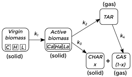
Figure 1.
Chemical kinetic scheme for fast pyrolysis of biomass [7,47].
All the reactions are assumed to be irreversible first-order, while the dependence of the specific reaction rate on temperature is expressed by the Arrhenius equation:
where represents the rate constant of reaction m, is the activation energy of reaction m, and R is the gas constant. These coefficients for each reaction are detailed in Table 1. The link between the reaction rate of Equation (18) and the reaction coefficients follows the structure presented by Xue et al. [12,13].

Table 1.
Reactions and kinetic parameters [51].
The ratios of CHAR in relation to the products CHAR+GAS () for reaction 3 for , , and are , and , respectively.
It is worth mentioning that the product yield depends on several factors, such as the geometry, the operating conditions, the material proportions, the physical and numerical modeling approaches, and, very importantly, the kinetic model adopted. This work seeks to contrast the relative importance of these variables, including the simplified kinetics adopted.
2.3. Numerical Approach
The previous set of equations forming the multifluid model for thermal reactive and particulate flow is addressed in the framework of the Finite Volume Method (FVM). The chemical kinetics and thermal fluid dynamics equations are solved in a segregated manner by a time-splitting procedure. To solve the fluid dynamics, SIMPLE-based algorithms are adopted for pressure–velocity coupling [52,53], and the partial elimination algorithm is used for multiphase momentum coupling [54].
In this work, 3 distinct phases are addressed (gas, sand, and biomass), which interact with each other by exchanging mass, momentum, and energy, each one consisting of multiple species, allowing chemical reactions between them. For the simulations, the suites OpenFOAM(R) v11 [16] and ANSYS Fluent(R) v18.1 [27] were used. General conclusions from the use of both are drawn later on in the Results Section, and, in general, both codes preserve the following structure:
- Establish the initial conditions for each phase variable.
- Compute the phase fractions based on phase-continuity equations but for the continuous phase (gas). Then, calculate the gas-phase fraction by subtracting the solid-phase fraction from unity.
- Obtain the drag and heat transfer coefficients between phases based on the stored values of the variables.
- Compute the granular viscosity of each phase and granular pressure.
- Compute the temperature field of each phase based on each phase’s energy balance.
- Compute the species fraction based on each species’ transport equation considering the reaction rates obtained from the new temperature fields.
- Compute the velocity field prediction of each phase based on the momentum equation.
- Construct and compute the shared pressure field based on the mass and momentum equations.
- Update the velocity field of each phase based on the new pressure field and flux reconstruction. This step can be iterated with the previous one in OpenFOAM following the PISO method.
- Iterate from 2 to favor the coupling between equations until a convergence criterion is reached and proceed with the next time step.
In the following tests, the results shown will be those given by OpenFOAM by default unless otherwise specified.
2.4. Test Cases
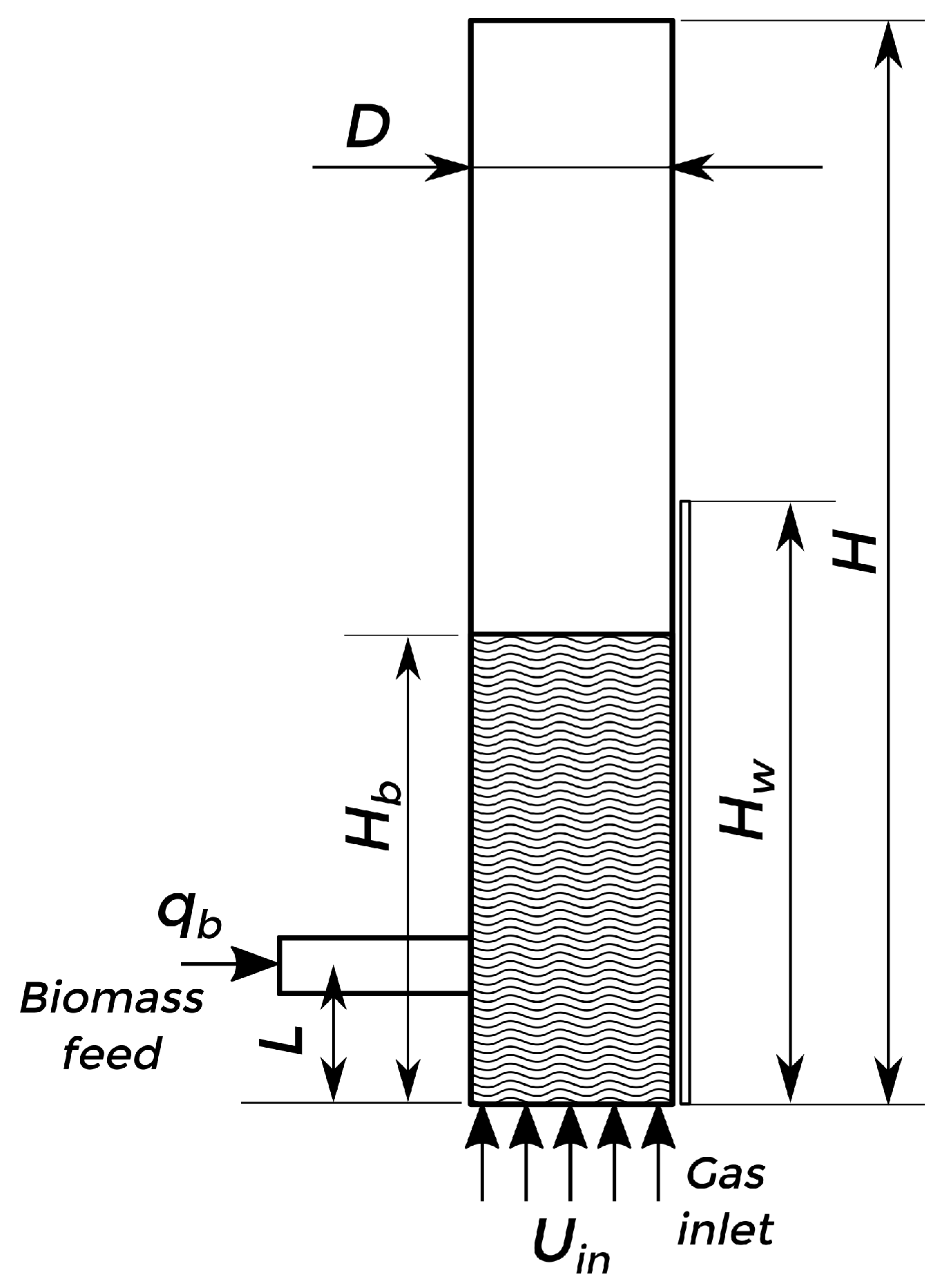
The described model was used to simulate lab-scale and pilot plant bubbling fluidized-bed reactors for the fast pyrolysis of biomass. Two experimental setups were considered for the simulations: Setup 1 [13], a lab-scale experiment, and Setup 2 [55], a pilot plant experiment. The scheme of the arrangement is shown in Figure 2, and the dimensions are detailed in Table 2. For both cases, three phases are considered: sand (solid), biomass (solid), and gas. The biomass (with a density of kg/m3 and a mean particle diameter of μm) is fed at 300 K into the reactor from the side at a fixed mass flow rate (), with differences in the initial composition (using red oak for Setup 1 and bagasse for Setup 2). At the same time, a bed of silica sand particles (with a density of kg/m3 and a mean particle diameter of μm) at an initial packing of 0.58 is fluidized by nitrogen injection at 773 K from the bottom of the bed at superficial velocity. The heated walls of the reactor (with a height from the bottom) are kept at a fixed temperature of 773 K to allow the fast pyrolysis reaction. The rest of the material properties are detailed in Table 3.

Figure 2.
Fluidized-bed reactor scheme.
Table 2.
Experimental setup and operating conditions (from [13,55]).
Table 3.
Species properties.
Regarding the numerical setup, the outlet conditions are specified at the top of the reactor; Johnson–Jackson partial slip boundary conditions for the solids [39] are adopted at the walls with a null gradient for the temperature, except for part of the heated wall (up to ). The inlet conditions for the gas (pure nitrogen) are imposed at the bottom, and the inlet conditions for biomass and nitrogen are dense packing conditions through the lateral feed. Most simulations were run until 100 s to allow statistical stationary conditions for averaging, and quasi-hexahedral cells were adopted. A mesh sensitivity analysis was performed to define the grid refinement in the following section.
3. Results and Discussion
This section focuses on the use of the computational model to address the test cases described in the previous section and draw conclusions about the adoption of the mass, momentum, thermal exchange, and kinetic models. The influence of each one of these models will be described in terms of the product yield and the field distribution inside the reactor and will be compared to the experimental data available. In order to do so, first, an adjustment of the numerical and geometrical setup (grid refinement, 2D vs. 3D approach, numerical schemes, and time steps) was performed, seeking an optimal balance between the computational cost and accuracy of the solution.
3.1. Numerical and Geometrical Setup
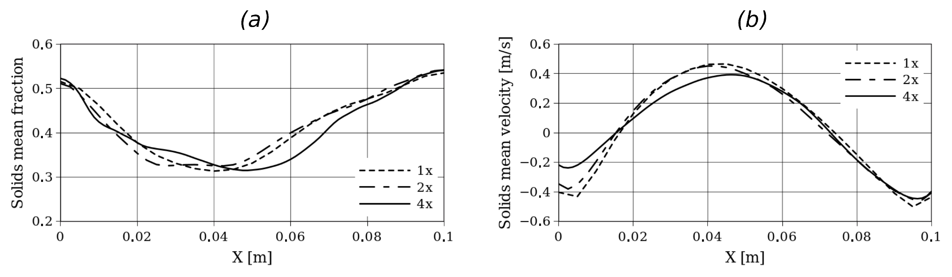
Initially, a grid refinement analysis was performed to define the mesh adopted for each case. For this purpose, Setup 2 was considered, and simulations were performed with grids of (1x), (2x), and (4x). Figure 3 shows the time-averaged solid velocity and volume fraction in a horizontal plane at cm from the bottom. On the other hand, Figure 4 shows the time-averaged solid volume fraction along the y-axis and time-averaged pressure along the y-axis. For all the simulations, second-order schemes and linear interpolation were used for the time and convective term discretization. For the adopted grid size, a time step of s was used to obtain numerically stable solutions.
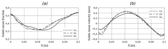
Figure 3.
Time-averaged solids fraction (a) and solid velocity (b) at y = 15 cm from the bottom for Setup 2 and for different grid refinements.

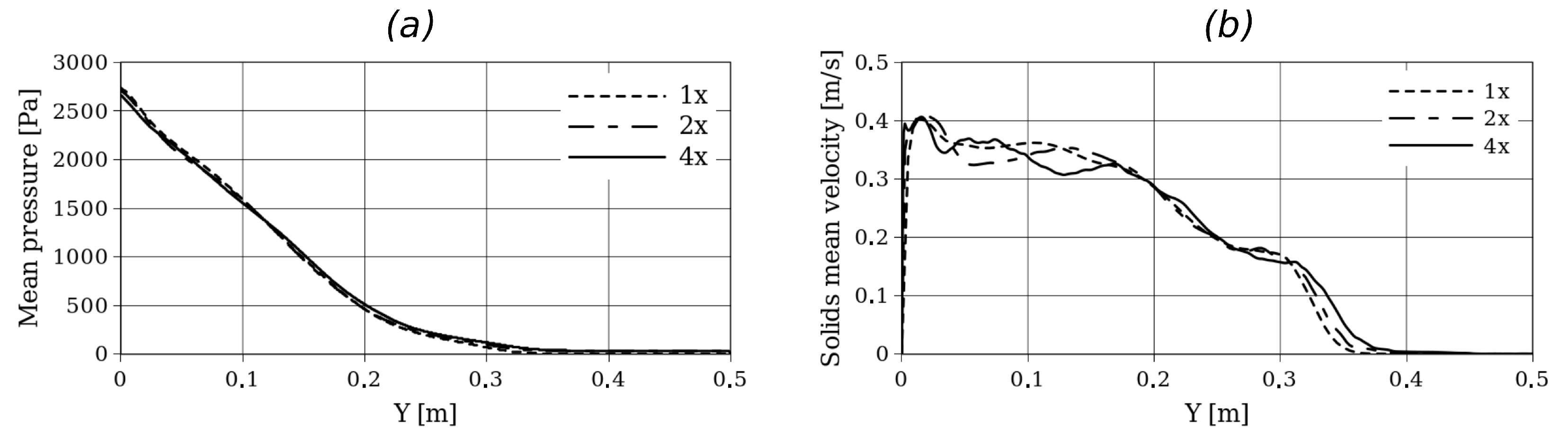
Figure 4.
Time-averaged pressure (a) and solid fraction (b) in a vertical center line for Setup 2 and for different grid refinements.
Here, small differences in the hydrodynamic profiles can be observed, especially near the left wall where the biomass enters the reactor. However, in terms of bed expansion, no significant differences are observed between the different grid refinements.
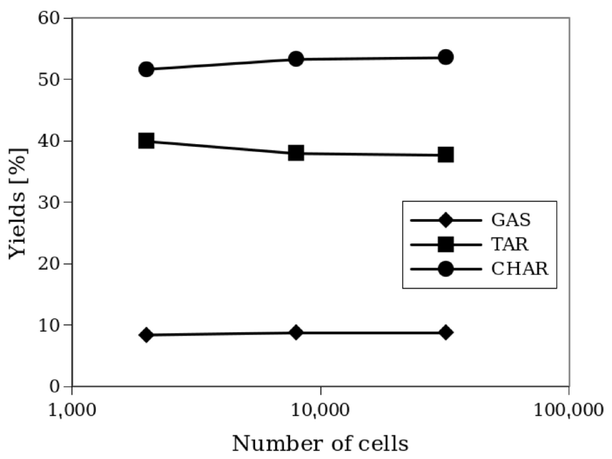
Despite these slight differences, the chemical conversion given by reaction products, as shown in Figure 5, reveals that the grid refinements have no significant impact on the product yields (see Equation (20)):
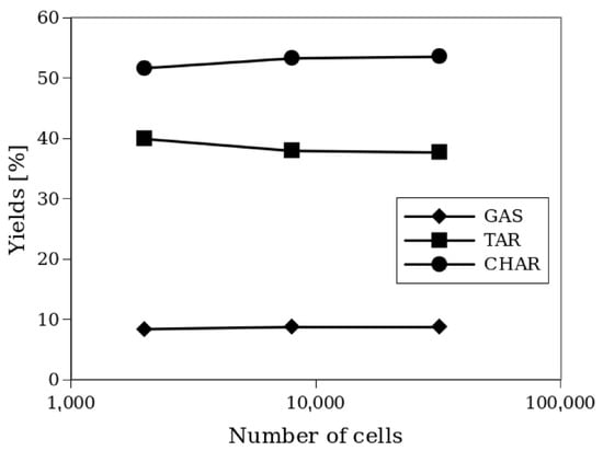
Figure 5.
Yields of the products of the process for different grid refinements.
It is worth noting that the 2x and 4x refinements produce very similar results. For this reason, the 2x refinement, corresponding to hexahedral cells of approximately 2.5 mm, was adopted for subsequent simulations. The same grid size was used for Setup 1. For a medium-sized grid (2x), a comparison with a 3D simulation was performed, giving differences of <2% in the yield values between 2D and 3D simulations. This was also observed by Xue et al. [13] for Setup 1.
3.2. Thermal and Momentum Coupling Models
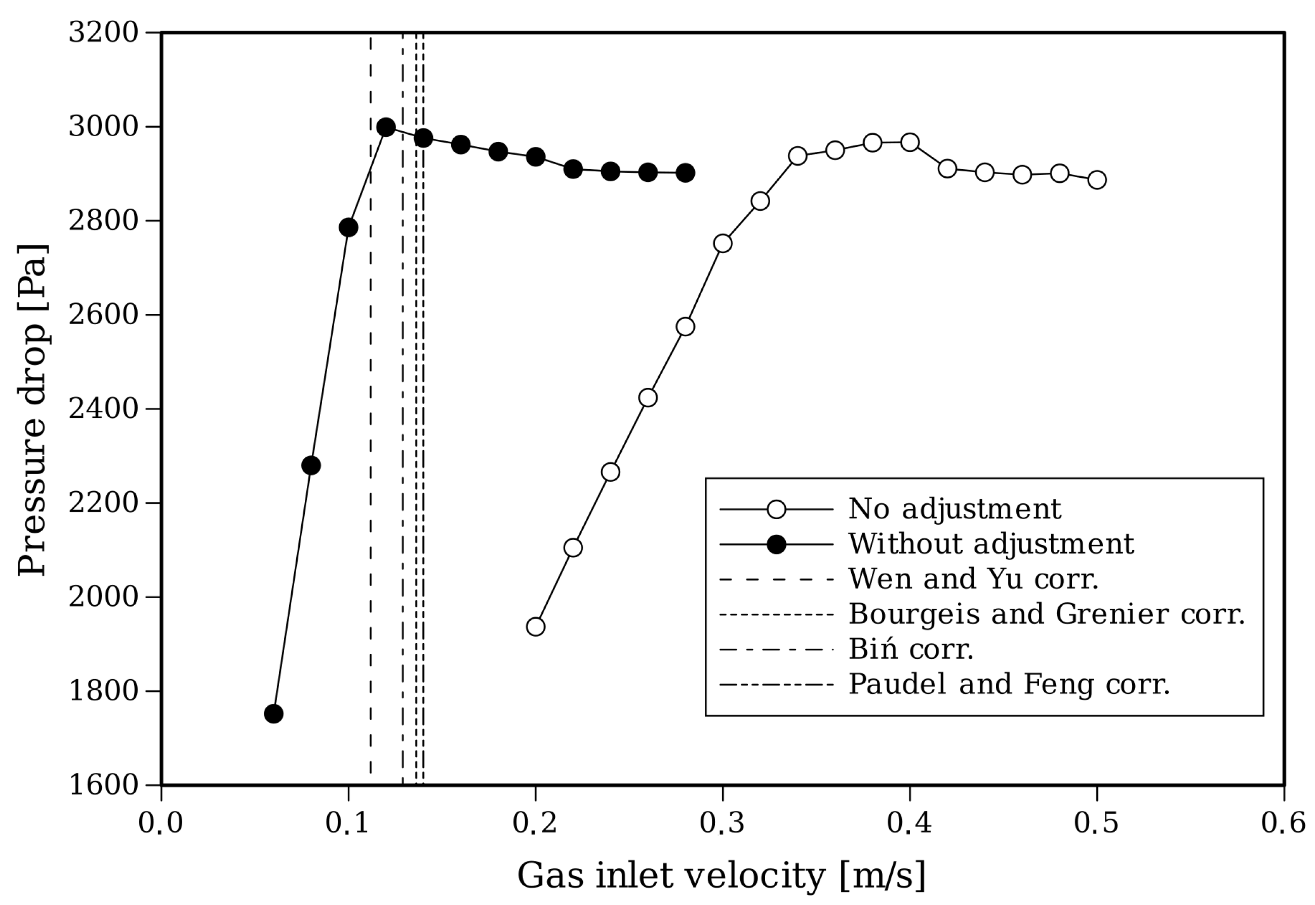
An important aspect to take into account for setting up the simulation is that the start of the fluidization process is affected by the temperature [56,57]. Therefore, the drag law needs to be adjusted for these conditions. Figure 6 shows the fluidization curves of the pressure drop for different gas inlet velocities and for standard values of the Syamlal–O’Brien drag coefficients and modified coefficients (, ).
For this approach, an adjustment of the drag model is performed following the methodology given by [58]. Along with these curves, in Table 4, the values of predicted by different correlations of the Wen–Yu family [33] that are apt for gas-particle flows under the current operating conditions [59] are shown. The adjusted drag law predicts a in accordance with the correlations and was adopted for the following simulations.
Here, , where all the parameters without subscripts refer to continuous phase properties.
Table 4.
Minimum fluidization velocity correlations for gas-particle flows.
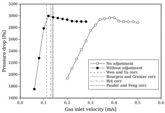
Figure 6.
Fluidization curves with CFD based on a Syamlal–O’Brien drag model with and without the adjustment of the coefficients and curves predicted by correlations [33,60,61,62].
Figure 6.
Fluidization curves with CFD based on a Syamlal–O’Brien drag model with and without the adjustment of the coefficients and curves predicted by correlations [33,60,61,62].
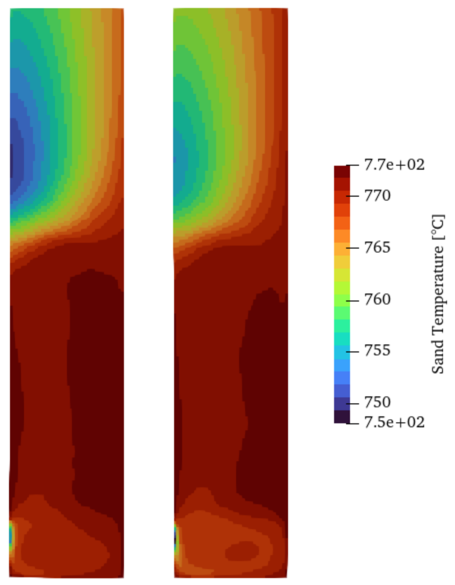
Another aspect to take into account is the heat transfer between phases. There are several correlations to account for this, with the Ranz–Marshall and Gunn model being among the most adopted correlations. Figure 7 shows the time-averaged sand temperature field (over 50 s after the first 5 s when the fluidization process begins). The temperature distribution for both cases shows hot spots close to the heated wall and a cold region in the upper part of the reactor where the gas phase is mostly present and close to the wall where the cold biomass is injected. The temperature of the sand has a direct influence on the reaction rates and, therefore, the product yields of the pyrolysis. However, as shown in Table 5, using both setups, the product yields do not change significantly between heat transfer models, which indicates a lack of sensitivity to this aspect for the overall products of the pyrolysis process.
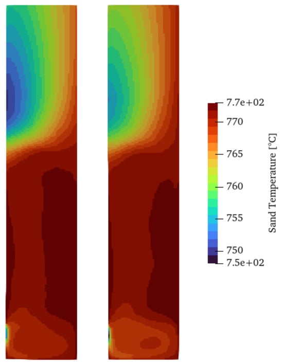
Figure 7.
Time-averaged solid temperature using the Ranz–Marshall (left) and Gunn (right) heat transfer models for Setup 2.
Table 5.
Yields of products for Gunn and Ranz–Marshall heat transfer models.
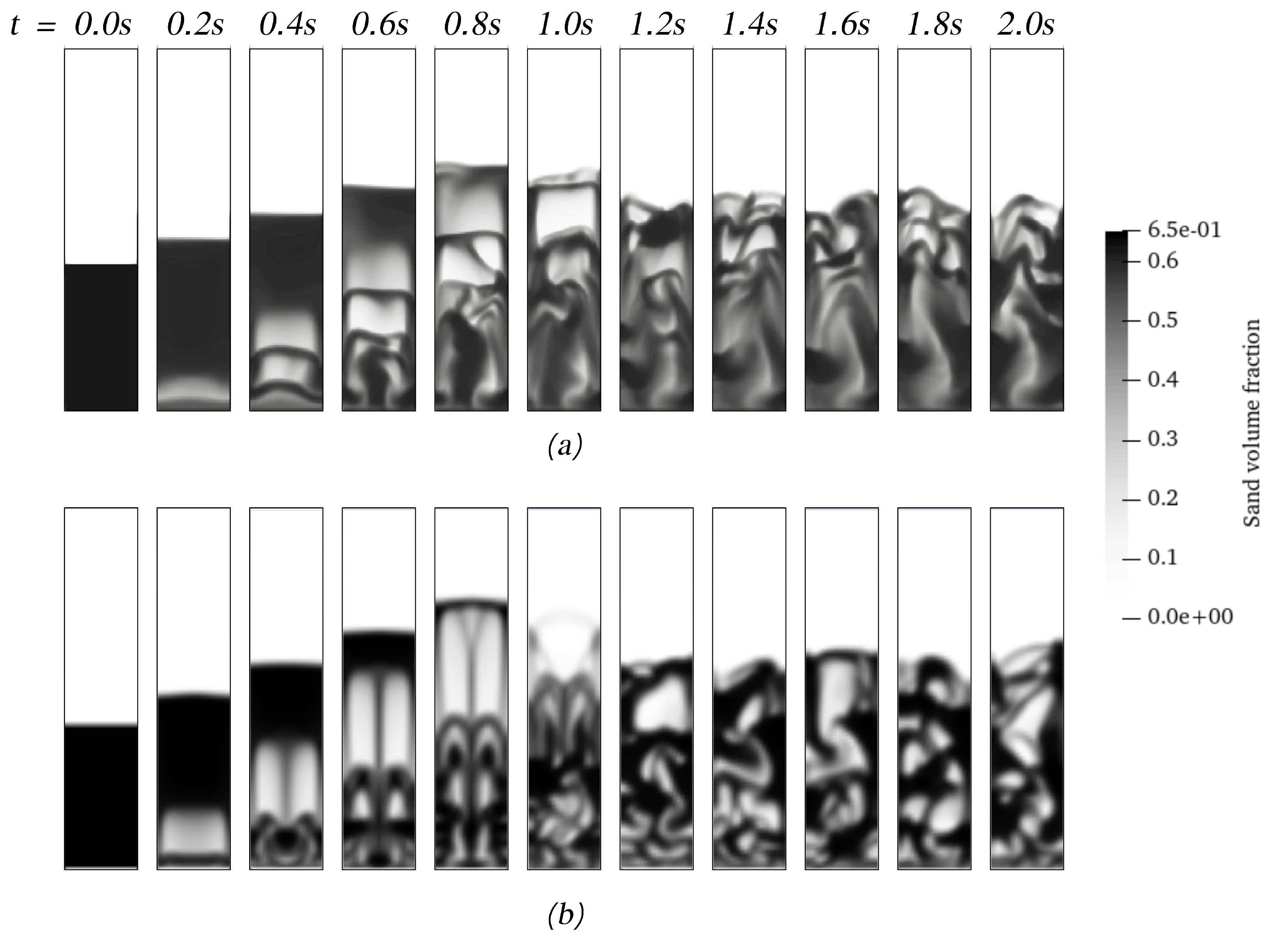
Another aspect to consider for CFD users is the computational program adopted for simulating these types of processes. ANSYS Fluent(R) and OpenFOAM(R) are two of the most well-known computational codes used for chemical reactor simulations. The first one is a proprietary code, but most parts of the general algorithm can be retrieved from the user’s manual [27]. There are many differences between codes in terms of the general algorithm and its implementation. Therefore, it is worth comparing the performance between codes to address the computational simulation of the process. Figure 8 shows the start of the fluidization using both codes, where it can be observed that, despite using the same interphase models, the solid distribution and the general hydrodynamic behavior differ from each other. ANSYS Fluent shows well-defined bubbles with a symmetrical evolution until the first bubbles erupt. On the other hand, OpenFOAM shows more diffusive interphases between pure gas and pure solids. Nonetheless, the yields of the products predicted with both codes, as shown in Table 6, have no significant differences. Moreover, the comparison is extended for both setups, resulting in differences of less than 3%.
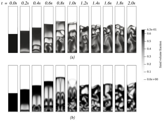
Figure 8.
The start of the fluidization process of sand and biomass using OpenFOAM (a) and ANSYS Fluent (b).
Table 6.
Yield values of the products using different computational codes and experiments.
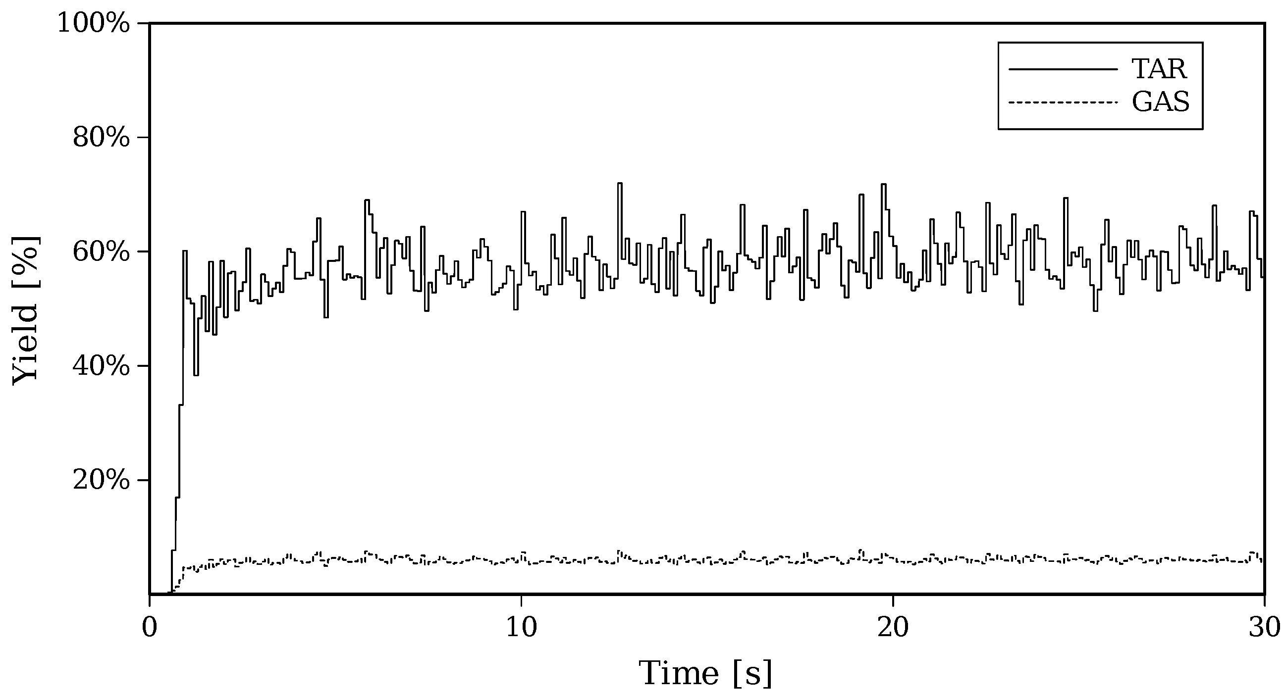
Figure 9 shows the transient evolution of GAS and TAR distributions for Setup 2, where it can be appreciated that after the first 5 s, a statistically steady rate of GAS and TAR production is reached.

Figure 9.
Transient evolution of yields of TAR and GAS for Setup 2.
The results shown up to this point demonstrate the lack of sensitivity of the yield of the products of pyrolysis to the thermal and hydrodynamic models, as well as the computational codes and numerical setups. However, the yield predictions still differ from the experimental results, for example, in the TAR production (as shown in Table 6), which suggests that other modeling aspects, such as the kinetic model and coefficients, should be considered.
3.3. Model for Chemical Kinetics
In Figure 10, the yields obtained for Setup 2 through simulation are presented, considering different values of kinetic parameters for secondary TAR–GAS degradation [51,63,64,65,66,67,68]. Each kinetic model was implemented and tested in both codes (OpenFOAM and ANSYS Fluent), and the results did not significantly change, so the same conclusions can be drawn for both software programs.
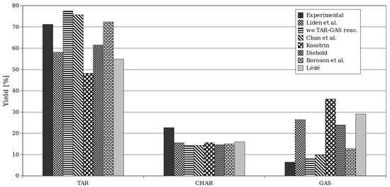
Figure 10.
Yields of products for different chemical kinetics using ANSYS Fluent for Setup 2 [51,55,64,65,66,67,68].
It can be observed that the original kinetic model given by the coefficients of Liden et al. [51], as listed in Table 1, generally underestimates the formation of TAR, the predominant product in the studied case of fast pyrolysis. Consequently, the predicted CHAR and GAS yields are generally higher than the experimental values (as shown in Table 6).
Fagbemi et al. [63] provided a set of kinetic parameters for reaction 4 (TAR to GAS), which are used in this section to study the effects of different kinetic parameters on secondary TAR pyrolysis. It is observed that excluding reaction R4 leads to an overestimation of TAR and GAS production and a corresponding underestimation of CHAR production. The yield results for different kinetic parameters for reaction 4 are shown in Table 7.
Table 7.
Kinetic coefficients for reaction 4 and yields of products for simulations with Setup 2.
Regarding CHAR production, the simulation results are lower than those obtained by Montoya et al. [55] in all cases shown in the table. However, the kinetic parameters from Chan and Krieger [64] and Boroson et al. [67] provide a better prediction of TAR generation. The CHAR yield is consistently underestimated, while the GAS yield is overestimated. Based on this observation, it can be concluded that the proportions suggested for primary pyrolysis to produce GAS and CHAR in reaction 3 might be the cause of the discrepancies between the model predictions and the experimental results. A detailed exploration and adjustment of the kinetic models is still needed to improve the prediction of CHAR production for the process.
Due to the improved predictions given by kinetic modeling (for example, using the coefficients from Chan and Krieger [64]), the same modification was made for Setup 1, as shown in Table 8. The results show a more accurate prediction of the yields of the products, especially for TAR and CHAR production.
Table 8.
Yields of products for simulations with Setup 1.
In any case, the results presented in this section highlight the a priori evident influence of chemical reaction kinetics, contrasting with the (not entirely obvious) lack of impact of thermo-hydraulic models and computational codes on the product yields of the fast pyrolysis process in bubbling fluidized beds.
4. Conclusions
This study focused on modeling the fast pyrolysis of biomass in fluidized-bed reactors using computational fluid dynamics (CFD) based on an Eulerian multifluid approach. Simulations were conducted to analyze the influence of various modeling parameters, including hydrodynamic models, heat transfer correlations, and chemical kinetics, on the yields of bio-oil (TAR), biochar (CHAR), and syngas (GAS). The numerical framework integrated both 2D and 3D geometrical setups and utilized OpenFOAM and ANSYS Fluent for cross-validation.
After performing a grid refinement analysis and adjusting the drag law for the corresponding operational conditions, the results demonstrated that hydrodynamic models and thermal correlations, such as heat transfer models, had a minimal impact on the predicted product yields. Similarly, no significant differences were observed in the product distributions between the computational codes used, emphasizing the robustness of the numerical setup. However, this study highlighted the critical role of chemical reaction kinetics in determining the distribution of pyrolysis products. Simplified kinetic schemes, although computationally efficient, consistently underestimated TAR production and overestimated GAS and CHAR yields when compared to experimental results.
To address these discrepancies, a detailed analysis of secondary TAR-GAS reactions was performed using different kinetic parameters. The findings showed that neglecting certain reactions, such as TAR-to-GAS conversion, led to the overestimation of TAR and GAS yields and the underestimation of CHAR production. Among the tested kinetic parameters, those proposed by Chan and Boroson provided better alignment with experimental TAR yields. Further work is still needed to predict CHAR production with higher accuracy. These results underscore the necessity of an accurate representation of primary and secondary reaction pathways for achieving reliable predictions.
Author Contributions
Conceptualization, C.M.V. and A.R.U.; methodology, C.M.V. and A.R.U.; software, C.M.V. and A.R.U.; validation, C.M.V. and A.R.U.; formal analysis, C.M.V., E.T., R.A.R., G.G.F. and A.R.U.; investigation, C.M.V. and A.R.U.; resources, G.M.; data curation, C.M.V. and A.R.U.; writing—original draft preparation, C.M.V. and A.R.U.; writing—review and editing, C.M.V., E.T., R.A.R., G.G.F., A.R.U. and G.M.; visualization, C.M.V. and A.R.U.; supervision, G.M.; project administration, G.M.; funding acquisition, G.M. All authors have read and agreed to the published version of the manuscript.
Funding
This research was funded by the following Argentine institutions: National University of Comahue (PIN 2022–04/I260); CONICET-National Scientific and Technical Research Council (PIP 2021–2023-11220200100950CO and PUE PROBIEN CO22920150100067); National Agency for the Promotion of Research, Technological Development, and Innovation and YPF Foundation (PICTO 2022-1410).
Data Availability Statement
The original contributions presented in this study are included in the article. Further inquiries can be directed to the corresponding author.
Conflicts of Interest
The authors declare no conflicts of interest.
References
- Ali, S.; Suboyin, A.; Haj, H. Unconventional and conventional oil production impacts on oil price-Lessons learnt with glance to the future. J. Glob. Econ. 2018, 6, 286. [Google Scholar]
- Armah, E.K.; Chetty, M.; Rathilal, S.; Asante-Sackey, D.; Tetteh, E.K. Lignin: Value addition is key to profitable biomass biorefinery. In Handbook of Biofuels; Elsevier: Amsterdam, The Netherlands, 2022; pp. 233–247. [Google Scholar]
- Babu, B. Biomass pyrolysis: A state-of-the-art review. Biofuels Bioprod. Biorefining Innov. Sustain. Econ. 2008, 2, 393–414. [Google Scholar] [CrossRef]
- Bridgwater, A.V. Review of fast pyrolysis of biomass and product upgrading. Biomass Bioenergy 2012, 38, 68–94. [Google Scholar] [CrossRef]
- Scott, D.S.; Piskorz, J. The continuous flash pyrolysis of biomass. Can. J. Chem. Eng. 1984, 62, 404–412. [Google Scholar] [CrossRef]
- Farrell, A.E.; Brandt, A.R. Risks of the oil transition. Environ. Res. Lett. 2006, 1, 014004. [Google Scholar] [CrossRef]
- Di Blasi, C. Modeling chemical and physical processes of wood and biomass pyrolysis. Prog. Energy Combust. Sci. 2008, 34, 47–90. [Google Scholar] [CrossRef]
- Papadikis, K.; Bridgwater, A.; Gu, S. CFD modelling of the fast pyrolysis of biomass in fluidised bed reactors, Part A: Eulerian computation of momentum transport in bubbling fluidised beds. Chem. Eng. Sci. 2008, 63, 4218–4227. [Google Scholar] [CrossRef]
- Bridgwater, A.V. Renewable fuels and chemicals by thermal processing of biomass. Chem. Eng. J. 2003, 91, 87–102. [Google Scholar] [CrossRef]
- Authier, O.; Ferrer, M.; Mauviel, G.; Khalfi, A.E.; Lede, J. Wood fast pyrolysis: Comparison of Lagrangian and Eulerian modeling approaches with experimental measurements. Ind. Eng. Chem. Res. 2009, 48, 4796–4809. [Google Scholar] [CrossRef]
- Lathouwers, D.; Bellan, J. Modeling of dense gas–solid reactive mixtures applied to biomass pyrolysis in a fluidized bed. Int. J. Multiph. Flow 2001, 27, 2155–2187. [Google Scholar] [CrossRef]
- Xue, Q.; Heindel, T.; Fox, R. A CFD model for biomass fast pyrolysis in fluidized-bed reactors. Chem. Eng. Sci. 2011, 66, 2440–2452. [Google Scholar] [CrossRef]
- Xue, Q.; Dalluge, D.; Heindel, T.; Fox, R.; Brown, R. Experimental validation and CFD modeling study of biomass fast pyrolysis in fluidized-bed reactors. Fuel 2012, 97, 757–769. [Google Scholar] [CrossRef]
- Syamlal, M.; Rogers, W.; O’Brien, T.J. MFIX Documentation: Theory Guide; Technical Note DOE/METC-95/1013 and NTIS/DE95000031; National Energy Technology Laboratory, Department of Energy: Morgantown, WV, USA, 1993. [Google Scholar]
- Xiong, Q.; Kong, S.C.; Passalacqua, A. Development of a generalized numerical framework for simulating biomass fast pyrolysis in fluidized-bed reactors. Chem. Eng. Sci. 2013, 99, 305–313. [Google Scholar] [CrossRef]
- Weller, H.G.; Tabor, G.; Jasak, H.; Fureby, C. A tensorial approach to computational continuum mechanics using object-oriented techniques. Comput. Phys. 1998, 12, 620–631. [Google Scholar] [CrossRef]
- Xiong, Q.; Yang, Y.; Xu, F.; Pan, Y.; Zhang, J.; Hong, K.; Lorenzini, G.; Wang, S. Overview of computational fluid dynamics simulation of reactor-scale biomass pyrolysis. ACS Sustain. Chem. Eng. 2017, 5, 2783–2798. [Google Scholar] [CrossRef]
- Zhong, H.; Xiong, Q.; Yin, L.; Zhang, J.; Zhu, Y.; Liang, S.; Niu, B.; Zhang, X. CFD-based reduced-order modeling of fluidized-bed biomass fast pyrolysis using artificial neural network. Renew. Energy 2020, 152, 613–626. [Google Scholar] [CrossRef]
- Houston, R.; Oyedeji, O.; Abdoulmoumine, N. Detailed biomass fast pyrolysis kinetics integrated to computational fluid dynamic (CFD) and discrete element modeling framework: Predicting product yields at the bench-scale. Chem. Eng. J. 2022, 444, 136419. [Google Scholar] [CrossRef]
- Wang, B.; Dai, J.; Li, S.; Lin, Y.; Patrascu, M.; Gao, X. Coupling coarse-grained DEM-CFD and intraparticle model for biomass fast pyrolysis simulation and experiment validation. AIChE J. 2024, 70, e18393. [Google Scholar] [CrossRef]
- Luo, H.; Wang, X.; Liu, X.; Wu, X.; Shi, X.; Xiong, Q. A review on CFD simulation of biomass pyrolysis in fluidized bed reactors with emphasis on particle-scale models. J. Anal. Appl. Pyrolysis 2022, 162, 105433. [Google Scholar] [CrossRef]
- Sia, S.Q.; Wang, W.C. Numerical simulations of fluidized bed fast pyrolysis of biomass through computational fluid dynamics. Renew. Energy 2020, 155, 248–256. [Google Scholar] [CrossRef]
- Makkawi, Y.; Mohamed, B. CFD modeling of date palm (Phoenix dactylifera) waste fast pyrolysis in a fluidized bed-including experimental kinetics, validation, and remarks on the modeling approach. Renew. Energy 2024, 224, 120175. [Google Scholar] [CrossRef]
- Pourhoseinian, M.; Asasian-Kolur, N.; Sharifian, S. Comparative computational fluid dynamics analysis of fast pyrolysis of agricultural feedstocks across different biomass categories. Biomass Bioenergy 2024, 180, 107026. [Google Scholar] [CrossRef]
- Chen, T.; Ku, X.; Lin, J.; Ström, H. CFD-DEM simulation of biomass pyrolysis in fluidized-bed reactor with a multistep kinetic scheme. Energies 2020, 13, 5358. [Google Scholar] [CrossRef]
- Shi, X.; Liu, H.; Zhang, X.; Lan, X.; Gao, J. Numerical simulation on effects of biomass type on its fast pyrolysis in fluidized bed reactor. Ind. Eng. Chem. Res. 2023, 62, 17100–17108. [Google Scholar] [CrossRef]
- Fluent Inc. Fluent Manual; Fluent Inc.: New York, NY, USA, 2003; Volume 6, pp. 14–16. [Google Scholar]
- Ishii, M. Thermo-fluid dynamic theory of two-phase flow. NASA Sti/Recon Tech. Rep. A 1975, 75, 29657. [Google Scholar]
- Enwald, H.; Peirano, E.; Almstedt, A.E. Eulerian two-phase flow theory applied to fluidization. Int. J. Multiph. Flow 1996, 22, 21–66. [Google Scholar] [CrossRef]
- Syamlal, M.; Gidaspow, D. Hydrodynamics of fluidization: Prediction of wall to bed heat transfer coefficients. AIChE J. 1985, 31, 127–135. [Google Scholar] [CrossRef]
- Syamlal, M. The Particle-Particle Drag Term in a Multiparticle Model of Fluidization; Technical Report; EG and G Washington Analytical Services Center, Inc.: Morgantown, WV, USA, 1987. [Google Scholar]
- Yang, N.; Wang, W.; Ge, W.; Li, J. CFD simulation of concurrent-up gas–solid flow in circulating fluidized beds with structure-dependent drag coefficient. Chem. Eng. J. 2003, 96, 71–80. [Google Scholar] [CrossRef]
- Wen, C.; Yu, Y. A generalized method for predicting the minimum fluidization velocity. AIChE J. 1966, 12, 610–612. [Google Scholar] [CrossRef]
- Gibilaro, L.; Di Felice, R.; Waldram, S.; Foscolo, P. Generalized friction factor and drag coefficient correlations for fluid-particle interactions. Chem. Eng. Sci. 1985, 40, 1817–1823. [Google Scholar] [CrossRef]
- Loha, C.; Chattopadhyay, H.; Chatterjee, P.K. Assessment of drag models in simulating bubbling fluidized bed hydrodynamics. Chem. Eng. Sci. 2012, 75, 400–407. [Google Scholar] [CrossRef]
- Lun, C.; Savage, S.; Jeffrey, D.; Chepurniy, N. Kinetic theories for granular flow: Inelastic particles in Couette flow and slightly inelastic particles in a general flowfield. J. Fluid Mech. 1984, 140, 223–256. [Google Scholar] [CrossRef]
- Savage, S. Analyses of slow high-concentration flows of granular materials. J. Fluid Mech. 1998, 377, 1–26. [Google Scholar] [CrossRef]
- Schaeffer, D.G. Instability in the evolution equations describing incompressible granular flow. J. Differ. Equ. 1987, 66, 19–50. [Google Scholar] [CrossRef]
- Johnson, P.C.; Jackson, R. Frictional–collisional constitutive relations for granular materials, with application to plane shearing. J. Fluid Mech. 1987, 176, 67–93. [Google Scholar] [CrossRef]
- Jenkins, J.T.; Savage, S.B. A theory for the rapid flow of identical, smooth, nearly elastic, spherical particles. J. Fluid Mech. 1983, 130, 187–202. [Google Scholar] [CrossRef]
- Gidaspow, D. Multiphase Flow and Fluidization: Continuum and Kinetic Theory Descriptions; Academic Press: Cambridge, MA, USA, 1994. [Google Scholar]
- Sinclair, J.; Jackson, R. Gas-particle flow in a vertical pipe with particle-particle interactions. AIChE J. 1989, 35, 1473–1486. [Google Scholar] [CrossRef]
- Srivastava, A.; Sundaresan, S. Analysis of a frictional–kinetic model for gas–particle flow. Powder Technol. 2003, 129, 72–85. [Google Scholar] [CrossRef]
- Tardos, G.I. A fluid mechanistic approach to slow, frictional flow of powders. Powder Technol. 1997, 92, 61–74. [Google Scholar] [CrossRef]
- Ranz, W.; Marshall, W. Evaporation from drops. Part 1. Chem. Eng. Prog. 1952, 48, 141–143. [Google Scholar]
- Gunn, D. Transfer of heat or mass to particles in fixed and fluidised beds. Int. J. Heat Mass Transf. 1978, 21, 467–476. [Google Scholar] [CrossRef]
- Miller, R.S.; Bellan, J. A generalized biomass pyrolysis model based on superimposed cellulose, hemicelluloseand liqnin kinetics. Combust. Sci. Technol. 1997, 126, 97–137. [Google Scholar] [CrossRef]
- Corbetta, M.; Pierucci, S.; Ranzi, E.; Bennadji, H.; Fisher, E. Multistep kinetic model of biomass pyrolysis. In Proceedings of the XXXVI Meeting of the Italian Section of the Combustion Institute, Procida, Italy, 13–15 June 2013; pp. 13–15. [Google Scholar]
- Ranzi, E.; Corbetta, M.; Manenti, F.; Pierucci, S. Kinetic modeling of the thermal degradation and combustion of biomass. Chem. Eng. Sci. 2014, 110, 2–12. [Google Scholar] [CrossRef]
- Bradbury, A.G.; Sakai, Y.; Shafizadeh, F. A kinetic model for pyrolysis of cellulose. J. Appl. Polym. Sci. 1979, 23, 3271–3280. [Google Scholar] [CrossRef]
- Liden, A.; Berruti, F.; Scott, D. A kinetic model for the production of liquids from the flash pyrolysis of biomass. Chem. Eng. Commun. 1988, 65, 207–221. [Google Scholar] [CrossRef]
- Patankar, S.V.; Spalding, D.B. A calculation procedure for heat, mass and momentum transfer in three-dimensional parabolic flows. Int. J. Heat Mass Transf. 1972, 15, 1787–1806. [Google Scholar] [CrossRef]
- Issa, R.I. Solution of the implicitly discretised fluid flow equations by operator-splitting. J. Comput. Phys. 1986, 62, 40–65. [Google Scholar] [CrossRef]
- Spalding, D. Numerical computation of multi-phase fluid flow and heat transfer. Recent Adv. Numer. Methods Fluids 1980, 1, 139–167. [Google Scholar]
- Montoya, J.; Valdés, C.; Chejne, F.; Gómez, C.; Blanco, A.; Marrugo, G.; Osorio, J.; Castillo, E.; Aristóbulo, J.; Acero, J. Bio-oil production from Colombian bagasse by fast pyrolysis in a fluidized bed: An experimental study. J. Anal. Appl. Pyrolysis 2015, 112, 379–387. [Google Scholar] [CrossRef]
- Subramani, H.J.; Balaiyya, M.M.; Miranda, L.R. Minimum fluidization velocity at elevated temperatures for Geldart’s group-B powders. Exp. Therm. Fluid Sci. 2007, 32, 166–173. [Google Scholar] [CrossRef]
- Reyes-Urrutia, A.; Venier, C.; Mariani, N.J.; Nigro, N.; Rodriguez, R.; Mazza, G. A CFD comparative study of bubbling fluidized bed behavior with thermal effects using the open-source platforms mfix and openfoam. Fluids 2021, 7, 1. [Google Scholar] [CrossRef]
- Syamlal, M.; O’Brien, T. The Derivation of a Drag Coefficient Formula from Velocity-Voidage Correlations; Technical Note; US Department of Energy, Office of Fossil Energy, NETL: Morgantown, WV, USA, 1987. [Google Scholar]
- Anantharaman, A.; Cocco, R.A.; Chew, J.W. Evaluation of correlations for minimum fluidization velocity (Umf) in gas-solid fluidization. Powder Technol. 2018, 323, 454–485. [Google Scholar] [CrossRef]
- Bourgeois, P.; Grenier, P. The ratio of terminal velocity to minimum fluidising velocity for spherical particles. Can. J. Chem. Eng. 1968, 46, 325–328. [Google Scholar] [CrossRef]
- Biń, A.K. Prediction of the minimum fluidization velocity. Powder Technol. 1994, 81, 197–199. [Google Scholar] [CrossRef]
- Paudel, B.; Feng, Z.G. Prediction of minimum fluidization velocity for binary mixtures of biomass and inert particles. Powder Technol. 2013, 237, 134–140. [Google Scholar] [CrossRef]
- Fagbemi, L.; Khezami, L.; Capart, R. Pyrolysis products from different biomasses: Application to the thermal cracking of tar. Appl. Energy 2001, 69, 293–306. [Google Scholar] [CrossRef]
- Chan, R.; Krieger, B. Modeling of Physical and Chemical Processes During Pyrolysis of a Large Biomass Pellet with Experimental Verification. Prepr. Pap. Am. Chem. Soc. Div. Fuel Chem. (United States) 1983, 28, 5. [Google Scholar]
- Kosstrin, H. Direct formation of pyrolysis oil from biomass. In Proceedings of the Specialists Workshop on Fast Pyrolysis of Biomass, Copper Mountain, CO, USA, 19–22 October 1980; pp. 79–104. [Google Scholar]
- Diebold, J. The Cracking Kinetics of Depolymerized Biomass Vapors in a Continuous; Colorado School of Mines: Golden, CO, USA, 1985. [Google Scholar]
- Boroson, M.L.; Howard, J.B.; Longwell, J.P.; Peters, W.A. Product yields and kinetics from the vapor phase cracking of wood pyrolysis tars. AIChE J. 1989, 35, 120–128. [Google Scholar] [CrossRef]
- Lédé, J. The cyclone: A multifunctional reactor for the fast pyrolysis of biomass. Ind. Eng. Chem. Res. 2000, 39, 893–903. [Google Scholar] [CrossRef]


Disclaimer/Publisher’s Note: The statements, opinions and data contained in all publications are solely those of the individual author(s) and contributor(s) and not of MDPI and/or the editor(s). MDPI and/or the editor(s) disclaim responsibility for any injury to people or property resulting from any ideas, methods, instructions or products referred to in the content. |
© 2024 by the authors. Licensee MDPI, Basel, Switzerland. This article is an open access article distributed under the terms and conditions of the Creative Commons Attribution (CC BY) license (https://creativecommons.org/licenses/by/4.0/).