Experimental Study of Wave Processes in Main Gas Pipelines under Normal Operating Conditions

Abstract

The article presents the results of processing non-emergency pressure measurements that are transmitted via the SCADA hardware and software system to the control center of the main gas pipeline. SCADA is widely used for real-time control of the modes of gas transmission systems. However, the data provided by SCADA contain some information that is not fully analyzed. The performed processing of pressure measurements is a passive experiment aimed at a deeper understanding of the flow processes that occur during the flow of gas in industrial pipelines of high power. As a result of the experiment, four types of wave phenomena were found: single waves of (a) compression and (b) decompression that were both damped as they moved along the pipe, (c) oscillations with an amplitude and frequency practically unchanged in a fixed section within a period of about 2 h, and (d) wave phenomena with a sharply changing amplitude and frequency within a period of several minutes. The characteristics of wave processes, such as the speed of movement and the decreasing or attenuating amplitude of oscillations, were evaluated. For evaluation, models were built that take into account the specifics of information transfer procedures, namely, SCADA’s representation of continuous functions in a discrete form. The results obtained can be used as an additional tool for searching for leaks, such as in fistulas and unauthorized tie-ins, allowing us to more accurately separate the useful signal from the noise. The question is raised about the adequacy of the one-dimensional model for describing the flow processes in the zones of large gradients of regime parameters. The reasons for possible inadequacy and ways to overcome it are indicated.

1. Introduction

With the current importance of gas supply systems in the energy sector of industrialized countries, the modeling of flows in pipes attracts great interest. The greatest attention is given to the study of unsteady processes. This is explained by the fact that being close to a stationary mode during the operation of gas transmission systems (GTSs) is rare. The sources of disturbance are many and varied. These include:

• Changing consumption and maneuvering flows to meet changing demand for gas;
• Equipment failures (leaks, pipe breaks, and equipment malfunctions);
• Turning the units on and off;
• Hydrate plugs and deposits of condensate, sand, and sludge in the pipe cavity;
• Carrying out repairs;
• Regulation of the component composition (calorie content) of gas;
• Regulation of the amount of gas accumulated in pipes for operational control in daily and weekly cycles;
• Unauthorized gas extractions, etc.

The processes taking place in these situations differ in the rate and amplitude of changes in the flow parameters. Numerous mathematical models of gas flow have been proposed to take into account the specifics of the processes, scale, and structure of the GTS. The vast majority of publications on the issue under consideration are devoted precisely to the analysis of models from which consequences are derived about the physical effects of flow processes. In this paper, the opposite approach is used. The observed effects of the flow processes are analyzed and, as far as possible, the extent to which they fit into the existing ideas about the processes is revealed. The study is based on measurements of the mode parameters.

One of the discussed problems is the problem of the legitimacy of the one-dimensional model, which is usually used in the study of unsteady gas flows in industrial pipelines. The model was developed by using traditional methods of continuum mechanics and consists of two or three partial differential equations. These equations follow from the laws of the conservation of mass and energy and the law of momentum [1,2]. If temperature is not one of the significant factors affecting the flow, then the energy equation is not considered. In addition to undoubted physical laws, when forming a model, assumptions are made that are based on more shaky foundations. This includes the so-called quasi-stationarity hypothesis, a formula for determining the coefficient of hydraulic resistance.

The hypothesis of quasi-stationarity is that the friction resistance in the gas flow is assumed to be proportional to w², where w(x,t) is the gas flow velocity averaged over the pipe section, x and t are the spatial and temporal coordinates. The validity of the hypothesis has been established for stationary flows, but its extrapolation to unsteady flows has not been sufficiently confirmed through experimentation. Ultimately, the question of the limits of its applicability remains unanswered.

Pipeline hydraulics and hydrodynamics are essentially based on experimental research and on observations of the regimes of industrial pipelines. Empirical data are used to characterize the friction resistance. Friction resistance is represented as a product of several factors, one of which is the coefficient of hydraulic resistance λ, which is an empirical parameter. The large number and variety of formulas for λ indicates that the friction coefficient depends on several factors, the influence of which is difficult to reflect in a formalized model. The inconsistency in observations of industrial gas pipelines has repeatedly made it necessary to make refinements to the model. This again leads to the conclusion that to obtain an adequate model, it is necessary to rely on the current information about the regimes and on the measured values of the flow parameters. It follows from the foregoing that even models of stationary gas flow in pipelines need additional substantiation by binding to the actual flow regimes.

Let us examine the energy equation. When it is derived, a linear law (Newton’s formula) is usually adopted to calculate the heat flux from the pipe to the soil. The adequacy of this law is usually not questioned. There is another problem: the fundamental impossibility of accurately knowing the soil parameters, particularly the soil temperature and the heat transfer coefficient from the pipe to the soil, which should be known throughout the pipeline. The fundamental impossibility of obtaining this exact knowledge is due to the fact that the parameters change depending on the ambient temperature and humidity. The problem is not emphasized in publications, but it indicates the fundamental inexpediency of searching for a mathematically accurate flow model. In addition, it should also be taken into account that the one-dimensional model of flow through the pipe is also approximate, since the flow velocity due to friction changes not only along the length of the pipe, but also along the radius, decreasing from the axis of the pipeline to the pipe wall. Thus, current information about the flow (measurements of regime parameters) is a source for improving models and, more accurately, for reflecting the physical features of the gas flow.

These facts indicate that the problem of refining the hydraulic model needs further consideration. Additional studies are needed to penetrate deeper into the nature of unsteady gas flows. It should be taken into account that the organization of research on large gas pipelines requires careful preparation and installation of special measuring equipment. The question is whether all currently available resources are fully utilized. Trying to answer this question, we want to draw attention to the fact that the data on the regimes that are regularly received by the control centers are not used to the full extent, and it is possible to extract information that supplements the existing ideas about the physics of flow processes in main gas pipelines.

In recent years, new opportunities have appeared due to the qualitative improvement of the metrological equipment of gas pipelines. SCADA systems make it possible to collect and transmit to the control centers of GTSs huge amounts of information about the regime parameters of the gas flow. This information is used to track abrupt changes in regime parameters, indicating violations of the normal operation of technological objects. In the case of sudden changes, emergency automatics come into action, and the dispatching personnel take measures to stabilize the situation. However, the possibilities of the new generation of metrological support are not yet exhausted. In papers [3,4], it was shown that if we consider the entire set of measurements over a certain time interval, then we can obtain a more accurate idea of the processes occurring in pipelines. In [5,6], the results of the study of wave processes obtained by processing SCADA information about regime parameters were presented. In this work, larger amounts of data are used, and improvements are made to the data processing procedures. This makes it possible to clarify previous results, and to discover and analyze the processes that occur during the transportation of natural gas through powerful large-diameter pipelines that, as far as the authors know, have not been previously described in the scientific literature.

Our passive experiment provides an opportunity to make some comparisons between our obtained results and the previous results. It could be expected that the flow model developed decades ago for gas pipelines, built for gas pipelines of that time, would differ from the model that adequately describes the regimes in modern gas pipelines, which have an internal smooth coating and can transport large volumes of gas at a higher pressure. Indeed, there are certain differences. It could be expected that with relatively small changes to the pumping volume, the flow regimes can become close to stationary. However, as the processing of measurements of gas flow parameters has shown, the flow process is accompanied by unexpected phenomena. In the pipeline, single waves of compression and depression arise and move either with the flow or against it. Other wave phenomena were also observed. Moreover, the speed of the waves differed significantly from both the speed of sound and the speed of gas movement. Apparently, there are various causes of wave phenomena. It is possible that some waves can cause metal fatigue, leading to cracks and, eventually, failures such as pipe rupture.

In addition to the potential possibility of refining the mathematical model of the flow, the results of processing the actual regime information can also be used in other applications. It is possible that when pressure waves are used to search for leaks, such as fistulas, unauthorized tie-ins, etc., they will make it possible to more accurately separate the useful signal from the noise.

2. Model of Unsteady Isothermal Gas Flow

To describe flows in extended pipelines, it is customary to use one-dimensional models—systems of equations that relate the parameters of the gas flow as functions of spatial x and temporal t variables. These functions are parameter values averaged over the pipeline cross section. We are interested in flows where the gas flow parameters include pressure p(x,t) and velocity w(x,t). The temperature can be considered constant, T = const, since its change has practically no effect on the processes under consideration.

The model of unsteady isothermal flow is composed of the equations of continuity (conservation of mass) and momentum. Using variables that are traditional in continuum mechanics and have a clear physical meaning, we write the system in the form

$$\left\{\begin{array}{l}\frac{\partial \rho }{\partial t}+\frac{\partial \left(\rho w\right)}{\partial x}=0\\ \frac{\partial \left(\rho w\right)}{\partial t}+\frac{\partial }{\partial x}\left(p+\rho w^2\right)=-\rho g\frac{\mathrm{d}h}{\mathrm{d}x}-\frac{\lambda \rho }{2D}w\left|w\right|\end{array}\right.,$$

(1)

where p, ρ, and w are the pressure, density, and velocity of gas flow, respectively; D is the inner diameter of the pipe; h = h(x) is the altitude of the pipeline route above sea level; and g is the free-fall acceleration. System of Equation (1) is supplemented by the equation of state

$$\rho =p/zRT\prime ,$$

(2)

where R is the gas constant, z is the compressibility factor, and T is the gas temperature. The arguments of the function z are the average values of pressure and temperature over the pipeline section, z = z(p_over, T_over). Using Equation (2), Equation system (1) is reduced to two unknown functions p(x,t) and w(x,t). If f is the inner cross-sectional area, the mass flow $M=\rho fw$ can be introduced into the number of variables and be considered as the desired functions p(x,t) and M(x,t). In practice, they do not use mass, but commercial flow rate.

Note: Further, to obtain numerical results, it was necessary to reasonably choose the value of the coefficient λ, which is important for the study. It is easy to see that the flow regime falls into the zone of quadratic friction, where λ does not depend on Re (λ = const). This value was estimated according to the criterion of the best matching of the entire set of measurements during the computational experiment. In fact, the numerical value of λ was used only when comparing the actual regime with the calculated one.

As noted above, the concepts on which the derivation of Equation (1) is based are generally accepted in continuum mechanics and do not raise doubts. However, a few assumptions are added to these ideas that seem less convincing. Questions arise about the legitimacy of some of the assumptions made in the derivation and further transformations of Equation (1). Thus, we formulated five questions:

• In Equation (1), velocity pressure is often neglected, causing the term $\rho w^2$ to be omitted in the second equation since $\rho w^2\ll p$. This latter relationship is, indeed, fulfilled for gas velocity w, which takes place under normal conditions in industrial gas pipelines, but will the relationship of $\frac{\partial (\rho w^2)}{\partial x}\ll \frac{\partial p}{\partial x}$ be fulfilled?
• The term $\frac{\lambda \rho }{2D}w\left|w\right|$ in the second part of Equation (1) characterizes the friction resistance. It was established empirically, based on observations of stationary flows, and was transferred without experimental confirmation to unsteady flows. How far is this hypothesis of quasi-stationarity from the truth? Should the model be corrected, and if so, how?
• Equation (1) does not include the energy conservation law. The temperature is assumed to be constant. When is the quasi-isothermal hypothesis valid?
• What approximations of the function z(p,T) can be considered acceptable?
• The coefficient of hydraulic resistance λ changes depending on x due to a change in speed and, consequently, the Reynolds number. Assuming it to be constant, we naturally introduce some errors. Can it be considered acceptable?

The answers to the questions posed can be obtained only by using actual data and by examining changes in the flow parameters in real gas pipelines. We must not forget about the changing conditions during the operation of industrial pipelines. The scale of production facilities has increased many times over: the length of pipelines and their diameters, the operating pressures, and the capacities of gas pumping units have increased. In connection with these changes, the models obtained many years ago require verification and, possibly, refinement. The fulfillment of this task is facilitated by the fact that the conditions for carrying out industrial experiments have significantly improved. Information complexes for monitoring the state of hydraulic structures are being continuously enhanced. The widespread introduction of SCADA systems for the automatic control of gas pipelines has made it possible to increase the efficiency of dispatching decisions and the level of safety of gas transport processes. However, the increased opportunities for obtaining more information on gas pipelines are not used to the full extent. To conduct some industrial experiments, in fact, it is not required to install additional devices; rather, it is enough to confine ourselves to regular metrological support.

Let us review publications that have discussed the problems of unsteady gas flow in long gas pipelines. There are many publications which touch upon issues close to the topic of this work, some of which are included in the list of references. Additional information can be found in reviews by [7,8,9], the first of which considered works up to the mid-1980s, and the other two which were written relatively recently.

Wave processes in a pipeline are widely used to detect leaks, as well as emergency situations caused by a pipeline rupture [10,11,12,13,14,15]. In cases of pipeline breaks, the task is to detect the emergency as quickly as possible, close the valves, and stop the flow to cut off the damaged section, thereby minimizing gas losses and the threat to people and the environment. The work of Modisette et al. [10] was one of the first to analyze pressure surges in a pipeline. The cause of the surge, in addition to the cause of emergency gas outflows, can be the sudden closing of the valve or the start/shutdown of the compressor. The modeling of flows in a pipeline makes it possible to distinguish between wave processes depending on the causes that generate them. Pressure surges can create problems for automatic safety shut-off valves. Valves should be calibrated to close automatically when a pipeline breaks, but not to respond to valve movement or compressor starting/stopping. This can be carried out based on the results of simulation of flow processes. Based on model calculations, the authors of [10] found, in particular, that as the pressure wave propagates, its amplitude decays, and the slope of the leading edge decreases due to friction or effects associated with compressibility. Later in this paper (Section 3), we present the results that confirm these facts to some extent and give quantitative characteristics of the process. However, no evidence of a change in the inclination of the leading edge was noted. From the analysis of various difference schemes for integrating the gas flow equations, it can be concluded that the results depend little on the finite difference scheme; instead, the influence of the mathematical model is more significant.

Barabanov and Lesnov [11] posed the problem of optimizing the number of pressure sensors. The installation of sensors requires considerable costs, as this process is associated with the need to upgrade telemetry systems. For a reasonable solution to the issue, effective methods for detecting leaks are needed, which are based on the detection of depression waves. Additionally, this, in turn, requires the development of methods for isolating a useful signal against a background of noise, the properties of which must be known. This paper will help to file signals other than those caused by breaks (or large leaks) in pipelines.

Modisette J.L. and Modisette J.P [12] also considered pressure surges moving through a pipeline. The phenomenon of the so-called digital diffusion (DD) was studied. DD is caused by the fact that when the equations are numerically integrated via difference methods, the jumps in the regime parameters are blurred. This effect is not due to physical causes, but is a consequence of a methodological error in the computational procedure. The task of the researcher is to develop a difference scheme and select the parameters of the procedure that correctly reflect the physics of the process. The practical significance of the work [12] lies in the fact that its results allow setting up automatic emergency shutdown valves.

Hanmer et al. [13], as well as the authors of [11,12], considered the problem of calibration of automatic valves. Adequate hydraulic modeling of fast transient processes requires a mathematical apparatus capable of describing the rarefaction wave in detail. A fast transient, in addition to the false operation of automatic shut-off valves, can also cause adverse effects on pipeline equipment, such as:

• The failure of fixed elements of the technical structure due to metal fatigue;
• The failure of dynamic elements leading to high loads on other elements;
• The failure of the pipeline due to exceeding the maximum allowable pressure.

Finally, bursts in high-pressure gas pipelines can lead, due to the Joule–Thomson effect, to very low temperatures near the hole from which the gas escapes. A low temperature leads to changes in the properties of the metal, making it more brittle. As a result, it becomes necessary to replace pipes not only in the vicinity of the fracture, but also that are a considerable distance from it.

Modisette and Hanmer [14] asked themselves how to distinguish the waves caused by a pipe rupture from those naturally occurring due to regular control actions such as, for example, scheduled compressor shutdowns, changes in stop valve settings during flow maneuvering, etc. The answer to this question is necessary to determine the correct settings for automatic pipe shut-off valves in an emergency. To solve the problem, experiments were carried out, the purpose of which was to estimate the damping rate of pressure waves. The results of the experiments made it possible to build adequate models and propose criteria to optimize the number of pressure sensors in the pipeline. The main problem in validating the model was the choice of an appropriate finite difference scheme. In [14], the results of integrating equations using three difference schemes were presented. The paper gives examples of how numerical solutions characterizing wave processes change depending on the choice of a difference scheme for integrating equations.

The listed publications show the relevance of the experimental study of wave processes in gas pipelines. The materials of such studies, among other things, make it possible to rationally build computational procedures and give an idea of the spectrum of possible wave processes, which is required to determine the optimal choice of metrological equipment for the GTS and calibration of control valves.

Interesting solutions to the equations of one-dimensional isothermal gas flow in pipes (system of Equation (1)) in the form of waves traveling at a constant speed were found by Gugat and Wintergerst [15]. However, such solutions were obtained under an initial condition of only a very specific type, and the answer to the question of whether these conditions can be provided by influencing the gas flow in a technically feasible way was not given in the article.

The substantiation of an adequate and easily implemented model for unsteady gas flows does not lose relevance over time. Moreover, the range of potential applications of the model is expanding. In connection with the expected development of hydrogen energy, the problems around the joint transport of hydrogen and natural gas are being actively studied [16,17]. Gong et al. [17] considered this problem as a special case in the flow of multicomponent mixtures. Its importance is growing due to the increasing use of LNG in conjunction with pipeline gases, nitrogen blending, and other similar technologies.

3. Experimental Study of Wave Processes in a Passive Experiment

3.1. Object of Conduct

As initial data, we used SCADA pressure measurements in normal modes on a linear section of the main gas pipeline (Figure 1). A two-line gas pipeline was considered. As shown in Figure 1, the lines connect the compressor plants (CPs) CP 1 and CP 2, and the distance between them is 176.9 km. Each CP has two compressor shops (CS): CS 1 and CS 2. For each line, the flow is from CS 1 to CS 2, (in Figure 1, the direction of the flow is indicated by a blue bold arrow). L_i gives the length of each section in km, the green valves are open, and the grey valves are closed. Connectors are installed along the route. In the area of the connectors, there are devices for measuring the regime parameters of the flow. We processed pressure measurements on the second line of those valves that are numbered in Figure 1.

Several records of regime parameters transmitted via the telemechanic system, from metering points to the control center of the gas transmission system, were studied. These records are time series of pressure values for 5–10 days with intervals between measurements of 1 min (the measured parameters also included temperature, but since temperature has a much smaller influence on the analysis results than pressure, data on the temperature regime were not processed). Pressure measurements p*(t) were processed using MeasureViewer computer technology (the MeasureViewer program was prepared for the analysis of the considered set of measurements by A.S. Balchenko) and MATLAB (Figure 2). Figure 2 shows the pressure waveform and some features of the pressure information transmitted by SCADA, which will be discussed in more detail in the next section.

3.2. Discreteness of Initial Information

Data on the gas flow regime parameters were collected along the route and transmitted to the dispatch control center by the SCADA system. They are the basis for monitoring the state of the pipeline and commercial settlements between consumers and suppliers. In the process of working with the SCADA system, various problems arose related to information distortions, data binding to calendar time, the consistency of operations, etc. Some of these problems are described in [18], including, in particular, examples of how incorrect data lead to errors in modeling production processes. We also had to face difficulties when working with SCADA information.

The physical quantity—pressure—is a continuous function of time p(t). The equipment—the telemechanic system (TS)—converts both the argument and the value of the function into a digital format by discretizing these variables. Figure 2 shows a fragment of the discretized function recording for a time interval of 100 min. The considered period contains 100 sessions of information transfer. Each period is divided into groups containing 8 + 39 + 1 + 52 = 100 measurements (see Figure 2). The first of these groups, eight measurements, is an interval of stable pressure. The next 39 measurements are the ascending branch of the graph, then the single measurement is the maximum pressure, and the last 52 measurements are the descending branch of the graph. Note that in the initial stable section, the instrument readings do not have to be equal. The TS is configured to work in such a way that the communication session starts when the inequality is met.

$$\left|p\left(t\right)-p\left(t_{i0}\right)\right|\ge h,$$

(3)

Here, p(t) is the current value of the pressure measurement, p(t_i0) is the pressure measurement transmitted via the TS during the last communication session, and h is the threshold value of the TS setting. According to this definition, at those moments of time when the discrete scale falls into the interval [t_i0, t] and when Equation (3) is not satisfied, information is not transmitted over the TS because it is considered that the value p(t) does not change. The “sparing” mode of operation of the TS introduces certain difficulties into the measurement processing procedure. Using the numerical data in Figure 2, we obtain an estimate of the discretization intervals with respect to the variables t and p. In total, 100 sampling steps in t correspond to 100 min of physical time, which means that the sampling step is $\delta t=1$ min. Due to the limited accuracy of the representation of points on the graph, even visually it can be determined that the distances between different pairs of points on the graph are slightly different from each other. Due to the same effect of limited precision in the representation of numbers, it is impossible to require absolutely identical estimates for the discretization step with respect to the variable p for different segments of the time series. Therefore, for the ascending branch of the graph in Figure 2, we obtained $\delta p\approx 0.119$ bar, and for the descending branch, $\delta p\approx 0.108$ bar. The pressure discretization step is closely related to the threshold value h introduced above, namely, $\delta p\approx h$.

The greater the accuracy of the source data, the more reasonable the conclusions that can be drawn from them. Even though the described method of data transmission reduces the accuracy, SCADA measurements provide new information, both of a qualitative nature and indicative of quantitative estimates. These are the questions that are discussed next. From the telemetry information, we managed to identify wave phenomena of four significantly different types: single compression waves, single depression waves, standing waves, and high-frequency fluctuations or chatter. To characterize wave processes, of interest are the speed of movement and the decrease or damping of the oscillation amplitude. These characteristics can be assessed directly from SCADA data. Along with this direct method, we also used another approach, the essence of which is the selection of a suitable analytical approximation of SCADA data and its subsequent analysis. It is not possible to determine a priori which of these approaches is better. The description of the second approach is contained in Appendix A.

3.3. Single Compression Waves

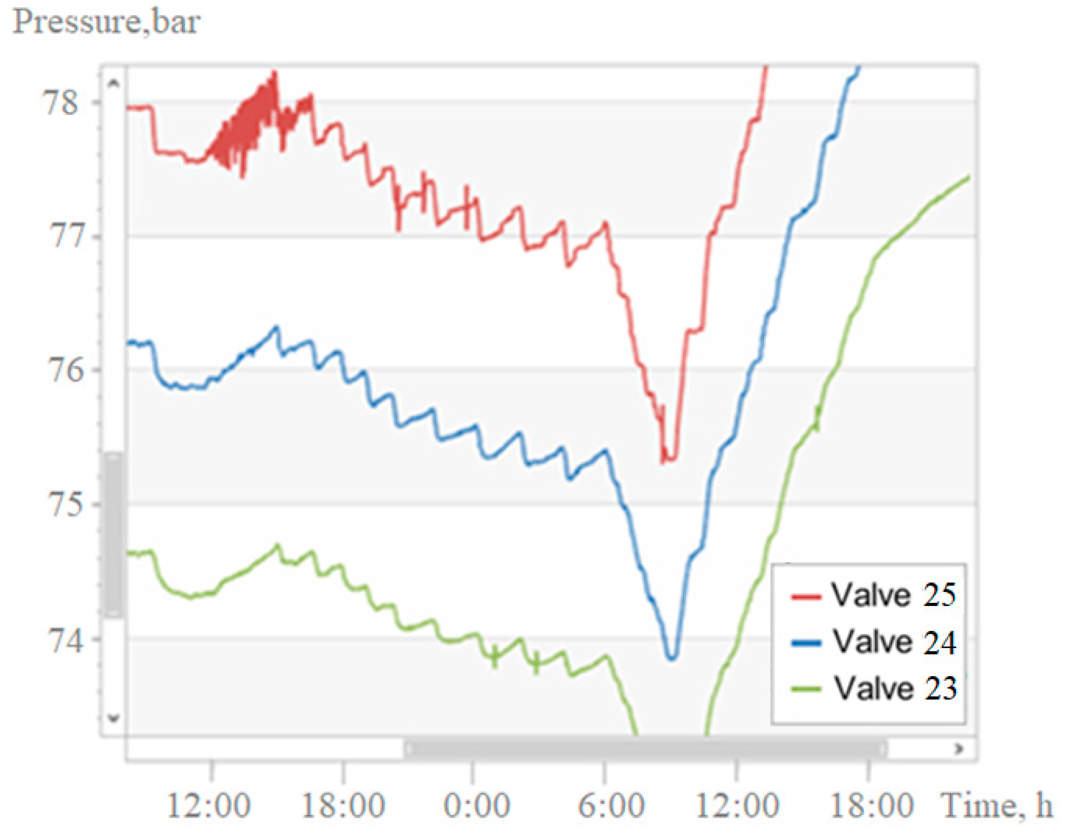
Of the four types of wave processes listed above, the waves of compression (increase in pressure) were encountered more often than others in the time series studied by us. Figure 2 shows a pressure-increasing wave recorded by one pressure gauge. Figure 3 shows the passage of a wave through several sequentially located measuring points. The source of perturbation for compression waves includes operations to control the modes of CP 2. The curves p(t) are built according to the readings of pressure gauges on the route of one of the pipeline lines (Figure 1). Reading curves in Figure 3 from bottom to top corresponds to the sequence of valve units against the gas flow (starting from CP 2): valve 5, valve 4, etc. The diagram shows how the compression wave moves through the pipeline. The amplitude of the pressure jump (about 3 bar on the lower curve) decreases to 1.5 bar with the passage of the wave to valve 1, and the pressure drops after the peak value changes from 1 bar at valve 5 to 0 at valve 1. The wave speed and the rate of decrease in its amplitude can be estimated knowing the distance between the valve nodes and the time it takes for the peak (maximum pressure) to pass from valve 5 to valve 1.

Let us set the goal to estimate the velocity of the compression waves and turn to examples 2 (Figure 4) and 3 (Figure 5). In these figures, pressure measurements transmitted via SCADA are shown as dots of different colors depending on the valve assembly (pressure gauge). The set of manometer i measurements is denoted by J(i). The discrete representation of a curve p_i(t), i.e., an ordered set of points $p_{ij}^{*}, j\in J\left(i\right)$ that represent the measurements, can be thought of as a vector $P_i^{*}=‖p_{ij}^{*}‖, j\in J\left(i\right)$.

The average speed $v_{ij}$ of the peak between the valves i and j can be estimated with the formula

$$v_{ij}=L_{ij}/(t_j-t_i),$$

(4)

where L_ij is the distance from the i to j valves, and t_j and t_i are the moments of passage of the peak of the valves j and i, respectively. In Equation (4), the value L_ij can be considered deterministic, that is, known exactly, and t_j and t_i are random, that is, quantities in the determination of which errors cannot be avoided. The error in determining the speed when other factors are equal will decrease as $\left|t_j-t_i\right|$ increases. In Figure 4, Figure 5, Figure 6 and Figure 7, dots represent the pressure measurements transmitted over the SCADA. Figure 4 clearly shows that when moving from the lower curve to the upper one, the maximum “blurs out”, that is, the error variance increases; moreover, even for the lowest curve (pressure measurements of valve 5) the moment of passage of the peak has significant uncertainty. Therefore, quite often, it is not possible to determine the moments of time t_j and t_i from the SCADA data. This is proposed to be carried out using a continuous approximation function. To represent a discrete sequence $P_i^{*}=‖p_{ij}^{*}‖, j\in J\left(i\right)$ through an analytical dependence, various methods of approximation were used. Some of them are presented in Equations (A2–A4). In Figure 4, Figure 5, Figure 6 and Figure 7, solid lines show the most successful approximations. We believe that such approximations improve the understanding of single waves and refine the parameters for estimating waves, and primarily, their velocity. For depression waves, these expectations were justified; for compression waves, they were not justified. Nevertheless, we considered it appropriate to provide information (in Figure 4 and Figure 5) for this case as well.

The compression wave gradually smooths out as it moves up against the current. Note that the pressure measurement graphs of the valves that are the first along the wave path (valve 5 in Figure 4 and valve 4 in Figure 5) have a pronounced asymmetry, approaching in shape the curve in Figure 2 (left).

It is natural to approximate such a curve on the ascending branch by a convex upward function, and on the descending branch, by a convex downward function. However, we did not use approximations of this type, since there are not enough SCADA data for this. In both cases (examples 2 and 3), the analytical approximations turned out to be unsuccessful. It is obvious that the crest of the wave and the maximum of its analytical approximation do not coincide. This is especially noticeable for valve 5 (Figure 4), valve 4, and valve 3 (Figure 5). For some cases, it is possible to compare the speed estimates from the SCADA information and approximation, as their closeness is evidence of the acceptable quality of the estimates. If the estimates are far from each other, then the estimate should be taken according to time and corresponding to the SCADA maximum pressure measurements, and the approximation should be considered unsatisfactory (the SCADA information for each valve is represented by dots in Figure 4, Figure 5, Figure 6 and Figure 7). In the situation in Figure 4, the curve p_i(t) of valve 1 in the vicinity of the maximum is quite flat: the maximum is not clearly defined. Therefore, in the procedure for determining the velocity of the compression wave, data for this valve in example 2 should not be taken into account. The processing of time series related to the propagation of compression waves (Figure 2, Figure 3 and Figure 4 and other cases) gave different estimates of the wave speed, which, however, do not go beyond 100–300 m/s.

3.4. Depression Waves

It follows from physical considerations that even an initially steep depression wave should become flat with time. This is exactly what took place in all the time series studied by us. For example, a depression wave was observed that propagated upstream from the inlet of CS 2 (CP 2), lasted about 40 h, and led to a decrease in pressure by more than 10 bar. The processing of telemetric information showed that, in contrast to the compression waves, depression waves are satisfactorily described by analytical approximations (A2–A4). This is clearly shown by comparing examples 4 (Figure 6) and 5 (Figure 7) with the examples of compression waves considered earlier.

As the graphs flatten out, the possibility of determining the extremum of a function $P_i^{*}=‖p_{ij}^{*}‖, j\in J\left(i\right)$ via its analytical approximation becomes more and more doubtful. Comparing the minima of discrete representations and their approximations, at the preliminary stage of information processing, we excluded graphs for valves 1 and 2 in example 5. For the remaining valves, the most reasonable estimate of the wave velocity is obtained from the data for the pipeline fragment between valves 5 and 4. The distance between the valves is 12.4 km. The average wave speed is, thus, about 200–250 m/s. Approximately, the same estimate is obtained for example 6.

3.5. “Standing” Waves

Along with mass phenomena—waves of compression and depression—two cases were recorded (Figure 8 and Figure 9) of an unexpected phenomenon: an oscillatory process that resembles standing waves. Standing waves are often associated with string vibrations. In liquid, they are observed in confined spaces and in open reservoirs. However, we do not know of cases of standing vibrations in industrial pipelines that have been described in scientific and technical periodicals.

Figure 8 shows a wave process that lasted about 16 h. During this time, nine cycles took place, of which the duration of each was approximately 108 min. Each cycle began with a sharp drop in pressure, followed by a relatively slower rise. A downward trend of about 1 bar in nine cycles was superimposed on the cyclic change in pressure. It is possible that the waves were initiated by the equipment switching at CP 1. The starting point of the process was a sharp decrease in pressure (by about 0.6 bar) after a stable regime. The oscillatory process ended with a significant (for valve 1, more than 2 bar) pressure drop. The time interval from the start to the moment of passage of the pressure minimum was approximately equal to 1 day.

Figure 9 shows a continuation of the same process as in Figure 8. The readings of three pressure gauges located downstream were recorded. Despite the discrepancy between the scales for both coordinates, the comparison of Figure 8 and Figure 9 allows us to draw some qualitative conclusions. As the group of “standing” waves moves forward, the wave amplitude decreases, and the pressure change becomes more gradual. Therefore, in order not to cause objections among the adherents of mathematical puritanism, we use quotation marks when applying the phrase “standing” to the phenomenon under consideration. At the last manometer in the direction of gas flow (lower curve in Figure 9), pressure fluctuations become almost imperceptible.

3.6. High-Frequency Fluctuations of Regime Parameters/Chatter

In this section, we do not consider fast processes such as, for example, shock waves moving at the speed of sound. It is unacceptable to draw any conclusions about such processes based on SCADA information. We also do not consider turbulent fluctuations. We classify as high-frequency processes those that are distinguished by a higher rate of change in parameters in comparison with the already considered processes of motion of solitary and “standing” waves.

In Figure 9, at the top left, you can see a graph depicting an aperiodic oscillatory process with a frequency much higher than the frequency of the “standing” waves discussed in the previous section. Here, we call processes of this kind high-frequency oscillations (HFOs). Since, due to the small scale, Figure 9 does not give an idea of HFOs, examples 7 and 8 are given for clarification. Figure 10 and Figure 11 present graphs of processes, or more precisely, fragments of processes where HFOs occur. Each figure has two parts. On the left-hand side, the graphs are plotted on a larger scale than in Figure 9, and on the right, they are plotted even larger, which allows you to view the same fragment of the time series on an enlarged scale.

It should be borne in mind that the time interval between communication sessions for SCADA is ≈1 min, and the period of the HFOs is less. Therefore, the pressure gauge readings transmitted via SCADA are, in fact, taken at random times. Examples 7 and 8 (Figure 10 and Figure 11), as well as numerous processed time series not shown in the article, indicate that at the beginning of the HFO process, the amplitude of oscillation increases, and at the end of the process it decreases. It is impossible to estimate the period of the HFOs according to the SCADA information, but there is no doubt that the phenomenon under consideration occurs quite often in the practice of operating gas pipelines. It is observed not in emergencies, but in normal modes. Data from some events with the HFOs that occurred in a relatively short time (an incomplete 3 months) are presented in

Table 1. Indicators of the processes of HFOs/chatter.

№	Calendar Date	Period	Duration, min	Valve	Amplitude, Bar
1	2016_04_08	12:55–13:00	5	1	0.5
2	2016_04_29	22:50–23:59	9	1	1.0
3	2016_05_30	17:28–17:34	6	2	0.3
4	2016_05_31	17:04–17:23	19	2	0.2
5	2016_06_01	18:53–19:17	24	3	0.8
6	2016_06_01	23:00–23:19	19	3	0.8
7	2016_06_02	19:32–20:14	42	3	0.7
8	2016_06_02	22:36–23:11	35	3	0.8
9	2016_06_03	12:38–12:46	8	2	0.25
10	2016_05_13	05:40–06:04	24	1	0.8
11	2016_06_16	05:40–06:04	24	2	0.4

. As can be seen, the events were recorded at different measuring points at different times of the day. Their duration is in the range from 5 to 42 min, with an average value of 19.5 min. The maximum oscillation amplitude lies in the range from 0.2 to 1.0 bar.

For the processes under consideration, we used the duplicate name chatter. The fact is that the true causes of the HFOs are unknown to us. It is possible that the pulsations in the pressure change record are the result of a malfunction or degradation of the instruments. To make the further discussion clearer, we formulate two hypotheses: H1—the considered type of records transmitted by the telemechanic system characterizes the physical process of transporting gas through a powerful gas pipeline; and H2—records appear due to the chatter of the pressure gauge and indicate malfunctions in the operation of the device under the current production conditions. Based on the information available, none of the hypotheses can be discarded. We can only talk about the probability that H1 is true and, consequently, H2 is unfair.

The performed analysis of telemetric information allows us to draw the following conclusions. If HFOs do occur in a gas flow (hypothesis H1 is valid), then:

• They cannot be considered small: this is evidenced by significant amplitudes of oscillations;
• HFOs quickly fade: not a single case of waves moving from one valve to another has been recorded;
• Fixed telemetry signals do not reveal the actual picture of the oscillatory process if the oscillation frequency exceeds the frequency of information transmission sessions by the SCADA system;
• An indirect confirmation of the H1 hypothesis is the fact that the amplitudes of the HFOs tend to increase at the beginning and decrease at the end (see Figure 10 and Figure 11), whereas chatter is usually characterized by an abrupt change in instrument readings from the minimum to maximum.

In any case, the study of the phenomenon under consideration must be taken seriously. If HFOs do occur in the gas flow (hypothesis H1 is valid), then they pose a threat to the integrity of the pipe. Rapid pressure fluctuations can lead to metal fatigue, and thus, it is possible that with large oscillation amplitudes the maximum allowable pressure may be exceeded. The chatter of pressure gauges (hypothesis H2 is true) can also lead to undesirable consequences due to the false operation of automatic shut-off valves.

3.7. Velocities of Single and “Standing” Waves

Wave speed is one of the most informative characteristics of the wave process. When studying wave processes, it is natural, first of all, to recall acoustic oscillations, i.e., the speed of sound. Another guideline is the gas flow rate (the physical speed of movement of gas particles). The mean velocity of gas particles is 10 to 20 m/s in the zone of parameters characteristic of the operating conditions of onshore gas pipelines. Both quantities—the speed of sound and the speed of movement of the transported product—are functions of pressure. Reference points for the characteristic conditions of operation of the gas pipeline under consideration can be considered the sound speed of the order of 400 m/s, and the flow velocity of 15 m/s. According to the above estimates of the velocities of single waves, both compression and depression depend on many factors, which, however, remain to be clarified. The main conclusion is that single waves move at speeds that are significantly greater than the flow velocity and significantly less than the speed of sound.

Single waves can move both along the gas flow and against it. The ordinate (“height”) of the maximum, which characterizes the wave amplitude, noticeably decreases with time, i.e., when moving from one measurement point to another. The scatter of the single wave velocity estimates obtained by us is quite large and is explained, first of all, by the inaccuracy of fixing the moments of time when its crest (for compression waves) or minimum (for rarefaction waves) passes through the measuring point, as well as by the blurring of the extremum due to the discreteness of pressure fixation.

In order to not give the impression that our estimates are too vague, firstly, we need to point out that these estimates were made for one gas transmission facility, and, secondly, we will provide some brief information about how the sound speed estimates differ. In numerous recent publications, the speed of sound is defined as

$$c_{sound}=\sqrt{zRT}$$

(5)

For example, Tijsseling and Vardy, in their work [19] devoted to wave processes in pipelines, connected the processes of wave propagation exclusively with the characteristics of the system of equations, which belongs to the hyperbolic type. More justified is the opposite approach that forms the equations in such a way as to adequately reflect the physical features of real processes. Only then can the consequences arising from the mathematical model be considered justified. The SCADA information is not suitable for describing waves propagating at the speed of sound, but it does allow us to state that other types of waves exist. The adequacy of models can be tested by how well the model describes these phenomena.

Formula (5) can serve as a guideline for determining the speed of sound waves, which are small oscillations when liquid and gases move in pipes. However, if a more accurate model is needed to determine the speed of sound, one should turn to continuum mechanics. With the help of this theory, the following formula is obtained for calculating the propagation velocity of small perturbations, which is applicable, therefore, for the calculation of $c_{sound }$ [2]:

$$c_{sound }=\sqrt{\left(C_p\left(p,T\right)/C_V\left(p,T\right)\right)\left(zRT/\left(1-\left(p/z\right){\left(\partial z/\partial p\right)}_T\right)\right)},$$

(6)

where $C_p\left(p,T\right)$ and $C_v\left(p,T\right)$ are the heat capacities of the gas at constant values of pressure and volume, respectively, and z = z(p,T) is the compressibility factor. Calculations using Formulas (5) and (6) were carried out with different approximations of z: in accordance with the American Gas Association standard $z\left(p,T\right)=1+0.257p/p_{cr}-0.533\left(p/p_{cr}\right)\left(T_{cr}/T\right)$, and with the Gazprom industry standard STO Gazprom 2-3.5-051-2006. Here, p_cr and T_cr are the critical values of pressure and temperature, respectively. The results of both calculations using approximations for z(p,T) turned out to be close. At pressures and temperatures varying in the ranges typical for the operation of most of the onshore gas pipelines, by using Formula (5) for c_sound, the boundaries of 486 and 512 m/s were obtained, and using Formula (6), 434 and 478 m/s.

Thus, the speed of propagation of single waves does not coincide with the speed of sound; instead, it is at least 40–50% less than the speed of sound. Let us note a certain similarity of solitary waves (surges) with solitons, which are waves in open channels that have attracted the attention of researchers for almost 200 years. As is known, solitons are a relatively rare phenomenon, and attempts to reproduce them experimentally have often ended in failure. The phenomena noted by us differ from that of the soliton due to a noticeable decrease in the oscillation amplitude with time.

“Standing” pressure waves propagate along the gas flow and against it. Estimates of the velocity of their propagation, made by the same methods as used for single waves, turned out to be more stable and equal to about 200 m/s. Stability is evidence of a greater reliability of the results and can be explained by the fact that the moments of achieving extreme values (maximum and minimum values) are less blurred here than in the case of single waves, and are determined with greater accuracy.

3.8. Some Methodological Questions

Thus, we have considered four types of wave phenomena observed in the operational modes of gas pipelines, of which two types of phenomena, in our opinion, have not yet been studied. However, wave processes occurring in gas pipelines are not limited to these four types. For example, in the already mentioned article by Modisette and Hanmer G. [14], the authors concluded that a sharp wave front does not dissipate when it moves along a gas pipeline. Among the waves of compression and depression that we analyzed, there were no examples when the wave would have a frontal character. Although this is not proof of the absence of such waves, it does indicate that they are relatively rare in normal gas pipeline regimes. Note that we are talking here about pressure fronts, since we have not considered temperature effects. In addition, the speed of the calculated wave fronts [14] was assumed to be equal to the speed of sound, whereas in all the observations we considered it was much less.

Without aiming to radically resolve the issue of the adequacy of Equation (1), we compared the actual (Figure 12 (left)) and calculated (Figure 12 (right)) flow regimes.

The calculations were performed using the VESTA software package (Gubkin Russian State University of Oil and Gas is the developer). We noted their common features. In both cases, the pressure wave moves against the gas flow with a gradual decrease in amplitude. However, the difference between the families of the actual pressure distribution and the solution of Equation (1) is also easy to notice. The actual blurring of the surge is much faster than in the model. It can be seen on the left of Figure 12 that when approaching the first measuring point along the gas flow (upper curve), the surge practically disappeared, and the pressure rose and stabilized. In the computational model (see Figure 12 on the right), although the magnitude of the surge decreases, the surge remains noticeable; thus, the pressure has not yet stabilized. In addition, the surge has the shape of a peak up to the second measuring point along the gas flow. In the model, an increasingly noticeable smoothing of the peak is observed. These deviations of the model indicate the incomplete adequacy of the model and the expediency of its improvement. The model flatly reflects the features of the process where the gradients of functions $\partial \rho \left(x,t\right)/\partial t, \partial p\left(x,t\right)/\partial x,$ etc are large.

Informatization of technological objects in gas transportation plays a certain role in the control of production processes, but its potential is far from being exhausted. The refinement of gas flow models in main pipelines will open up new opportunities for the automatic recognition of leaks and other emergency situations and will contribute to the improvement of the operational control of the gas transmission system as a whole.

Based on refined models of non-stationary processes, it is possible to develop new procedures for regime diagnostics. In order to track fluctuations arising for various reasons, the current regular information systems are suitable. Control and measuring devices and automation and telemechanics, which are equipped with main gas pipelines, ensure the receipt of huge amounts of information in real time, which, however, is not being fully used. It is not needed to directly solve the priority tasks of operational control, such as, for example, flow maneuvering. Due to the relative speed of the processes, a large amount of recorded data cannot be directly (that is, without appropriate preparation) used by the dispatching personnel. In practice, information technologies are also needed for the preliminary processing and analysis of incoming information to forecast the occurrence of emergency situations.

Relying on unused reserves of information, it is advisable to set new tasks, including, for example, the continuous monitoring of the tightness or dampener of strong disturbances. Recent advances in the field of information technology allow us to hope for the creation of the next generation of information systems that perform new functions.

4. Conclusions

This paper analyzed the graphs of pressure changes recorded by the entire complex of measuring points located on a main gas pipeline. Based on this representative information, the adequacy of mathematical models of non-stationary gas flow in long pipelines was verified in the first approximation. The results of the analysis made it possible to outline the following approaches for the correction (refinement) of the one-dimensional model of gas flow in order to more adequately describe real processes: the preservation of the often discarded term in the equation of momentum, and the rejection of the hypothesis of quasi-stationarity.

It has been established that under the operating conditions of loaded main gas pipelines, the following phenomena occur which were not previously described in the literature: sharp surges and drops in pressure propagating as solitary waves with a damped amplitude, wave ensembles resembling standing waves, and high-frequency oscillations or chatter. The velocities of solitary waves and periodic processes were estimated. The wide range of changes in the estimates was explained by the inaccuracy of the measurements, and by the discreteness of the pressure scale and of time-point fixation.

The observed wave propagation velocities are by an order greater than the speed of gas particles and approximately 40–50% less than the speed of sound. In addition to refining the mathematical model of the flow, the results of the passive experiment can be used to search for leaks due to holes, unauthorized tie-ins, etc. They will allow experts to more accurately separate the useful signal from noise when setting up automatic valves to shut off the gas pipeline in emergency situations.

The conducted passive experiment showed the possibility of the extended use of SCADA by means of an operational analysis of wave processes based on telemetric information received by dispatching control centers from gas transmission systems. In particular, it can be expected that such an approach will be useful when searching for leaks, when setting up automatic control valves for emergency valves, and when solving issues to improve metrological support. The use of SCADA to improve the integrity and safety of gas pipelines is recommended not instead of, but in addition to existing information systems. For the processing of SCADA information, original algorithms were developed that take into account the specifics of the processes of collecting and transmitting data on measurements of regime parameters.

Therefore, the observations made have led to the discovery of wave effects in the flow of gas in long pipelines, which have not been previously described in the scientific and technical literature. However, the problem of the more profound study of these effects, although posed, is not closed. It is necessary to identify the cause of the occurrence of “standing” waves and the factors that cause their sudden attenuation. An in-depth study of such a phenomenon of unknown nature, such as high-frequency oscillations or the chatter of devices, can also lead to constructive conclusions. If it turns out that this is indeed a wave process in the transported medium, then it remains to be investigated whether the vibrations are transmitted to the pipeline and whether they can affect the integrity of the pipe. SCADA information is not sufficient for such studies. Instead, the use of information technologies that provide a higher frequency of regime parameter fixing and are suitable for studying waves propagating at the speed of sound will be required.

The main issue left unanswered from those raised in the paper is the development of a mathematical model capable of adequately describing wave processes with large gradients of change in regime parameters. The established discrepancy between the solutions of the currently widely used model—a system of partial differential equations—and some features of wave processes revealed during observations indicates the presence of a problem which still needs to be investigated.

The results of the passive experiment indicate the expediency of conducting active experiments. When planning such experiments, it will be necessary to study the reaction of the production facility to regular management operations, such as switching compressors on/off, and the complete or partial blocking of the flow via the valves. During the experiments, it should also be possible to change the parameters of the gas flow in order to obtain more reliable information for correcting, if necessary, the flow model. An active experiment will ensure greater accuracy of the initial information in terms of fixing the moments of the beginning and end of the application of control actions. The results of the passive experiment will help to properly plan the active experiment. For this purpose, it is necessary to direct efforts to study the remaining unexplained phenomena that accompany regular transportation processes with a high load in large-diameter gas pipelines.