Numerical and Experimental Investigation of the Effect of Micro Restriction Geometry on Gas Flows through a Micro Orifice

Abstract

This study experimentally and numerically investigates the effects of the nozzle/needle distance (clearance) and supply pressure on single phase compressible gas flow in a micro orifice with needle restriction, which play important roles in many engineering applications such as cryogenic cooling and MEMS (microelectromechanical systems) device cooling. Nitrogen was used as the working fluid at supply pressures ranging from 10 to 50 bars, while the conical needle draft angle was 15°. The nozzle/needle distance (clearance) was changed from 100 µm to 500 µm. From the experimental point of view, the load provided by the working fluid over the needle was measured by a load sensor. For the numerical analysis, six turbulence models and three wall treatments were considered in numerical simulations. The effect of micro restriction on high-pressure micro-gas flows was further assessed by numerical modeling. It is evident from the results that the utilized turbulence model has a considerable effect on the computed results. The k–ε standard and Spalart–Allmaras models were found to be not suitable for modeling micro-scale gas flows with restriction. On the other hand, the k–ε realizable and k–ω SST models exhibit the best performance in predicting the results.

1. Introduction

The discovery of the Joule–Thomson effect (J–T effect) by Prescott Joule and William Thomson via proverbial porous plug experiment, where a piston-driven gas was forced through narrow orifices into a low-pressure environment, offered new lanes for advanced cooling systems [1]. An isenthalpic expansion of pressurized gas into ambient pressure leads to a sudden temperature drop of the working fluid. This phenomenon is known as the integral isenthalpic J–T effect [2]. Cryogenic cooling benefitting from the J–T effect has been widely studied. The integration of such advanced cooling systems into micro heat exchangers has become the center of research attention [3,4,5]. The increasing interest in J–T cooling systems with MEMS (microelectromechanical systems) devices arises from the advantageous characteristics of miniature J–T cryocoolers such as design simplicity, absence of moving parts, advanced durability, lower maintenance requirements, and cost effectiveness [6]. The rapid cooling ability combined with the compactness makes the use of miniature cryocooler devices favorable for integration into complex systems such as thermal cameras, infrared sensors, and missile homing heads with guidance systems and probes of cryosurgery. As the designs of miniature J–T cooling systems are taken into consideration, a variety of configurations can be found in the literature. However, the basic implementation can be summarized as the adjustment of the gas flow area exiting from a nozzle with the help of a flow restrictor, thereby realizing the isenthalpic expansion of high-pressure fluid through the throttling process [7].

The most crucial element determining the performance of this type of cryocooler is the heat exchanger. Hampson-type recuperative heat exchangers were widely used in such systems and were both numerically and experimentally examined in the literature [8]. The steady-state numerical analysis conducted by Chua et al. [9,10] and the transient analysis by Damle et al. [9] shed light on the optimization of innovative J–T cryocooler designs. Damle et al. [3] further improved the numerical analysis with the employment of finite reservoir capacity and the effect of the reservoir pressure. They observed that a large pressure variation in high-pressure region resulted in a significant temperature drop. Considering the development of primordial Joule–Thomson cryocooler devices, air was one of the most broadly used gases [11,12,13]. The experimentation of J–T cryocoolers with a singular type of gas such as nitrogen [14,15,16], helium [17], argon [18], hydrogen [19], or neon [20] was implemented in the following years and then followed by the inquisition of the expansion characteristics of the binary mixtures such as nitrogen–hydrogen [21,22], nitrogen–neon [23], or argon–helium [24]. Moreover, new emerging opportunities in microfabrication offered the ability of size reduction and microsystem integration for J–T cryocoolers, where microchannels and multi-stage chips were developed for such cooling systems [25,26]. Nowadays, innovative J–T cryocooler designs with unorthodox microfabrication techniques continue to emerge. For example, a ceramic miniature J–T cryocooler design fabricated via 3D printing was recently presented [26,27].

Recently, in order to reduce the cost of research efforts, numerical simulations have become more desirable. From the fluid dynamics perspective, new models have been developed for modeling single phase and phase change-based heat and fluid flow [28,29], including fluid solid interaction (FSI) [30,31] and aerodynamics [32]. In this regard, Dong et al. [33] provided a numerical model for presenting the choked mass flow characteristics of the helium fluid during the Joule–Thomson process. In another study, Baki et al. [34] proposed a one-dimensional model for the optimization of J–T heat exchangers.

Even though the performance evaluations of various J–T cryocooler designs were examined with different types of gases, there is still a lack of a parametric study on gas flows with a microflow restriction, where the effects of needle distance and supply pressure are assessed. In this regard, a fundamental understanding of the effect of gas flows with needle restriction exiting from micro-scale flow elements is necessary for providing a better design and performance. To fill this gap in the literature, an experimental analysis of the effect of the distance between the nozzle and needle (clearance) in micro-scale gas flows was performed. The supply pressure used in this study ranged from 10 to 50 bars. The force generated by nitrogen (N2) gas flows over the needle was measured by a load sensor. The needle restrictor was incrementally moved towards the micro orifice, and the output resistance (kΩ) recorded by the load sensor was converted into force (mN) for the flow restriction force analysis. Moreover, the literature lacks a comprehensive study on the effect of different turbulence models and their effect on the predicted results. Therefore, a numerical study was performed to examine the validity of different turbulence models and wall treatments on the predicted results. The purpose of the numerical and experimental analysis presented in this work is to enhance understanding about restricted gas flows and force exerted over the restrictor by the flow and to provide a reference study for miniature J–T cryocooler designs.

2. Experimental Studies

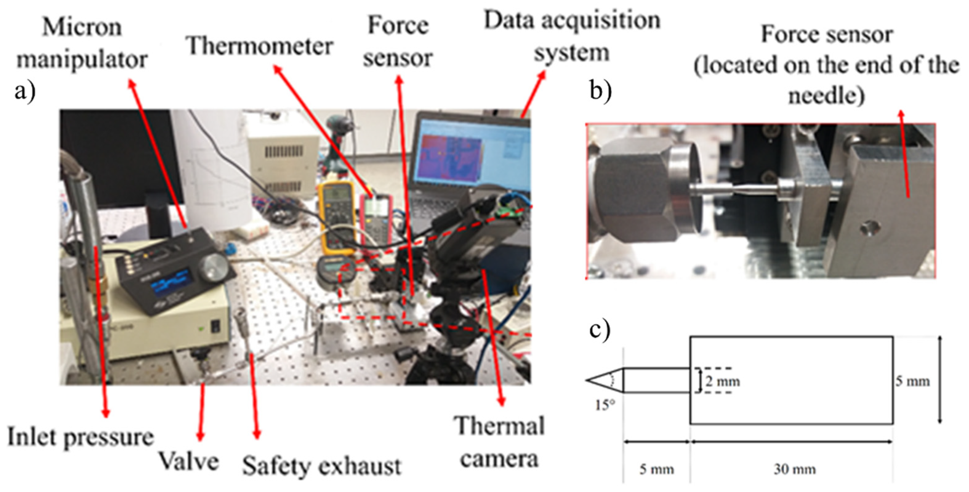
2.1. Experimental Setup and Components

The experimental setup, test section, and needle shape are presented in Figure 1. The experimental setup consists of a needle with 15° of draft angle, fine control valves (Swagelok, Solon, OH, USA), pressure sensors (Omega, Norwalk, CT, USA), a microfilter (Swagelok) safety valve, highly pressurized nitrogen gas (Linde Gas, Gebze, Kocaeli), a micro-manipulator (MP-225 Motorized Micromanipulator, Sutter Instrument), fittings (Swagelok), a micro-channel (Small Parts, Logansport, IN, USA), and a force-sensing resistor (Interlink Electronics, Camarillo, CA, USA). Moreover, a filter is included in the experimental setup. The aim of this filter is to avoid particles larger than a specific size (in this experimental setup 15 µm) in the flow. A pressure sensor is placed on the test section inlet in order to obtain the upstream pressure. Two start/stop valves for the control of the flow are employed in the experimental setup. The valve orifices are fully opened during the experimentation. The experiments are conducted on a tubular channel acting as an orifice. The inner diameter of the channel is 2 mm. The needle with specified geometrical properties shown in Figure 1c is used as the flow restrictive element. A force sensor is located at the end of the needle to obtain the force acting on the needle at different upstream pressures and clearances.

2.2. Data Reduction

The experimentally controlled parameters are the upstream pressure, restricting needle draft angle, and its distance from the orifice. During the experiments, the sole measured parameter is the force exerted on the restricting needle. The measurements are taken by a force-sensing resistor (FSR), which works as a load sensor. This sensor is located at the end side of the needle and is confined with an aluminum holder. The resistance values obtained from the FSR are pre-characterized by known external loads, (x-y) N with the incremental change of force in steps of 5 × 10⁻² N for high precision. The collected data are curve-fitted, and the resulting resistance vs. force profile is used for the force measurement and validation of the numerical results. The experimental uncertainties are presented in

Table 1. Experimental uncertainties.

Parameter	Uncertainties
Orifice diameter	±10 µm
Conical needle diameter	±10 µm
Resistance resolution	±0.5%
Resistance accuracy	±5–10%
Force measurement accuracy	±8–12%
Pressure drop	±1–3%
Micromanipulator motion resolution	±1 µm

.

3. Computational Studies

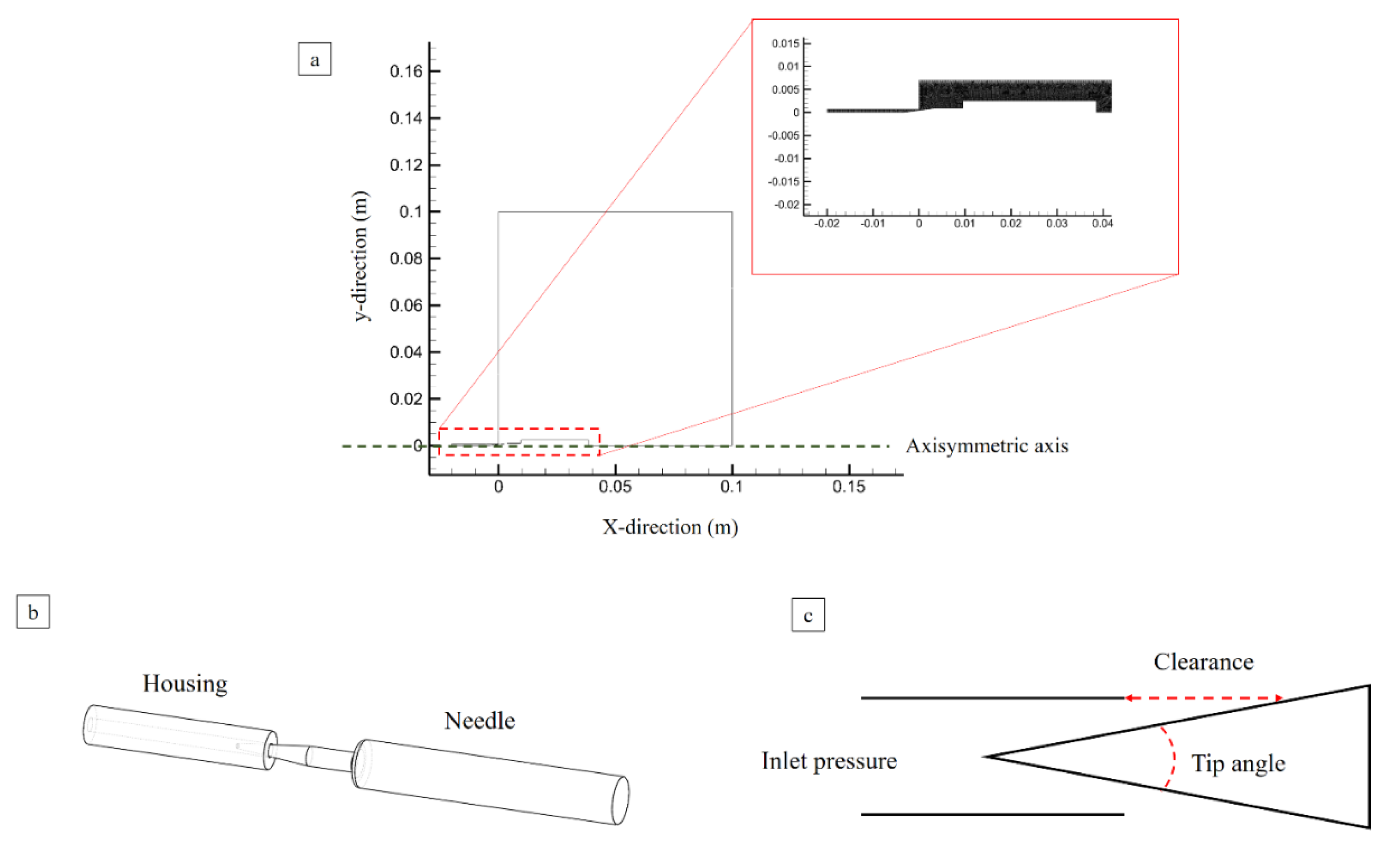
3.1. Computational

The governing equations, consisting of mass, momentum, and energy conservation, are solved using the finite volume approach with the software ANSYS Fluent 21.0. In order to model the steady-state turbulent compressible flow, a 2D axisymmetric domain is considered, and the Reynolds-averaged Navier–Stokes (RANS) equations are solved in the related domain. First order numerical schemes are implemented for the spatial discretization. Moreover, to evaluate the gradients, the least-squares method is used.

Since the governing equations are strongly interconnected, a density-based coupled solver, which solves them simultaneously and results in a faster convergence, is considered. The use of this algorithm requires setting up a Courant–Friedrichs–Lewy (CFL) condition, which is necessary for convergence while solving the governing equations. Considering a safety factor, CFL is considered as 0.1 to have a stable solution. Regarding the complex nature of the flow (high speed and compressible flow), in order to enjoy a relatively quicker convergence, a full multi-grid (FMG) initialization scheme is applied to the solving domain. The computational domain is shown in Figure 2a.

3.2. Numerical Analysis and Conservation Equations

Nitrogen is selected as the working fluid, and the thermophysical properties are obtained using the NIST (National Institute of Standards and Technology) real gas model [35,36]. Compressible nitrogen gas having inlet pressures ranging from 10 bar to 50 bar and a constant inlet temperature of 293 K are considered. Spatial and temporal resolutions are kept high in order to be able to solve the unsteady nature of the flow without the employment of turbulence modeling. The Favre-averaged form of the compressible Navier–Stokes equations are conducted due to the high variations in density of the flows. The governing equations are mass, momentum, and energy conservation. Their mathematical formulations are as follows, respectively:

$$\mathbf{\nabla }.\left(\mathit{\rho }\overrightarrow{\mathit{u}}\right)=\mathbf{0}$$

(1)

$$\mathit{\rho }\mathbf{\left(}\overrightarrow{\mathit{u}}.\mathbf{\nabla }\right)\overrightarrow{\mathit{u}}=-\mathbf{\nabla }\mathit{p}+\mathit{\rho }\overrightarrow{\mathit{g}}+\mathbf{\nabla }.\stackrel{\mathbf{=}}{\mathbf{\tau }}$$

(2)

$$\mathbf{\nabla }.\left(\left(\mathit{\rho }\mathit{e}+\mathit{p}\right)\overrightarrow{\mathit{u}}\right)=\mathbf{\nabla }.(\mathbf{\kappa }\mathbf{\nabla }\mathit{T}-{\displaystyle \sum }_{\mathit{j}}{\mathit{h}}_{\mathit{j}}{\mathit{J}}_{\mathit{j}}+\mathbf{\nabla }.\stackrel{\mathbf{=}}{\mathbf{\tau }})$$

(3)

Here, $\stackrel{=}{\tau }=\mu \left[\left(\nabla \overrightarrow{\mathit{u}}+\nabla \overrightarrow{\mathit{u}}\right)-\raisebox{1ex}{$2$}\!\left/ \!\raisebox{-1ex}{$3$}\right.\nabla .{\overrightarrow{\mathit{u}}}^{T}I\right]$ is the stress tensor, $e=h+\raisebox{1ex}{$p$}\!\left/ \!\raisebox{-1ex}{$\rho $}\right.+\raisebox{1ex}{${\left|\overrightarrow{\mathit{u}}\right|}^2$}\!\left/ \!\raisebox{-1ex}{$2$}\right.$, is the total energy, and I is the unity tensor matrix. Moreover, µ and ρ are the viscosity and the density of the working fluid, respectively. Moreover, $\overrightarrow{\mathit{u}}$ is the velocity vector, which can be decomposed into $u_r$ and $u_z$ components standing for the radial and axial velocities, respectively. In addition, g is the gravitational constant, and p is the pressure field.

It should be noted that at the inlet, a pressure inlet with zero velocity is considered, while the pressure outlet is considered at the outlet. Moreover, on the walls, the no-slip boundary condition is imposed.

3.3. Turbulence Models and Near Wall Treatments

Six RANS turbulence models are considered, namely: (i) Spalart–Allmaras, (ii) k–ε standard, (iii) k–ε realizable, (iv) k–ε RNG, (v) k–ω standard, and (vi) k–ω SST (see

Table 2. Summarization of the turbulence models.

Model	Expression
Spalart–Allmaras	$\frac{\partial }{\partial x_i}\left(\rho \tilde{v}{u}_i\right)=G_v+\frac{1}{{(P{r}_t)}_{\tilde{v}}}\left[\frac{1}{\partial x_j}\left\{\mu +\rho \tilde{v}\right\}\frac{\partial \tilde{v}}{\partial x_i}+C_{b2}{\left(\frac{\partial \tilde{v}}{\partial x_j}\right)}^2\right]-Y_v+S_{\tilde{v}}$
k–ε standard	$\frac{\partial }{\partial x_i}\left(\rho k{u}_i\right)=\frac{\partial }{\partial x_i}\left[\left(\mu +\frac{{\mu }_t}{{(P{r}_t)}_k}\right)\frac{\partial k}{\partial x_i}\right]+G_k+G_b-\rho \epsilon -Y_M+S_k$ $\frac{\partial }{\partial x_i}\left(\rho \epsilon u_i\right)=\frac{\partial }{\partial x_i}\left[\left(\mu +\frac{{\mu }_t}{{\left(P{r}_t\right)}_{\epsilon }}\right)\frac{\partial \epsilon }{\partial x_i}\right]+C_{1\epsilon }\frac{\epsilon }{k}\left(G_k+C_{3\epsilon }{G}_b\right)-C_{2\epsilon }\rho \frac{{\epsilon }^2}{k}+S_{\epsilon }$
RNG k–ε	$\frac{\partial }{\partial x_i}\left(\rho k{u}_i\right)=\frac{\partial }{\partial x_j}\left({\alpha }_k{\mu }_{eff}\frac{\partial k}{\partial x_j}\right)+G_k+G_b-\rho \epsilon -Y_M+S_k$ $\frac{\partial }{\partial x_i}\left(\rho \epsilon u_i\right)=\frac{\partial }{\partial x_j}\left({\alpha }_{\epsilon }{\mu }_{eff}\frac{\partial \epsilon }{\partial x_j}\right)+C_{1\epsilon }\frac{\epsilon }{k}\left(G_k+C_{3\epsilon }{G}_b\right)-C_{2\epsilon }\rho \frac{{\epsilon }^2}{k}-R_{\epsilon }+S_{\epsilon }$
Realizable k–ε	$\frac{\partial }{\partial x_j}\left(\rho k{u}_j\right)=\frac{\partial }{\partial x_j}\left[\left(\mu +\frac{{\mu }_t}{{\left(P{r}_t\right)}_k}\right)\frac{\partial k}{\partial x_j}\right]+G_k+G_b-\rho \epsilon -Y_M+S_k$ $\frac{\partial }{\partial x_j}\left(\rho \epsilon u_j\right)=\frac{\partial }{\partial x_j}\left[\left(\mu +\frac{{\mu }_t}{{\left(Pr\right)}_{\epsilon }}\right)\frac{\partial \epsilon }{\partial x_j}\right]+\rho C_1{S}_{\epsilon }-\rho C_2\frac{{\epsilon }^2}{k+\sqrt{\nu \epsilon }}+C_{1\epsilon }\frac{\epsilon }{k}{C}_{3\epsilon }{G}_b+S_{\epsilon }$$C_1=\max \left\{0.43,\frac{\eta }{\eta +5}\right\} \eta =S\frac{k}{\epsilon } S=\sqrt{2S_{ij}{S}_{ij}}$
Standard k–ω	$\frac{\partial }{\partial x_i}\left(\rho k{u}_i\right)=\frac{\partial }{\partial x_i}\left({\Gamma }_k\frac{\partial k}{\partial x_j}\right)+G_k-Y_k+S_k$ $\frac{\partial }{\partial x_i}\left(\rho \omega u_i\right)=\frac{\partial }{\partial x_j}\left({\Gamma }_k\frac{\partial \omega }{\partial x_j}\right)+G_{\omega }-Y_{\omega }+S_{\omega }$
SST k–ω	$\frac{\partial }{\partial x_i}\left(\rho k{u}_i\right)=\frac{\partial }{\partial x_i}\left({\Gamma }_k\frac{\partial k}{\partial x_j}\right)+{\tilde{G}}_k-Y_k+S_k$ $\frac{\partial }{\partial x_i}\left(\rho \omega u_i\right)=\frac{\partial }{\partial x_j}\left({\Gamma }_k\frac{\partial \omega }{\partial x_j}\right)+G_{\omega }-Y_{\omega }+D_{\omega }+S_{\omega }$

). These specified models have been comprehensively utilized in the literature. More information about these models can be found in the ANSYS Fluent theory guide [37].

3.4. Mesh Independency Analysis

In order to investigate the effect of grid number on the obtained results (on applied force, different grid numbers ranging from 6 × 10³ to 2.4 × 10⁶) is investigated. The realizable k–ε model and highest pressure are considered. As seen in

Table 3. Effect of grid numbers on predicted force.

Number of Grids	F (N)
6 × 103	22.9
2.5 × 104	23.4
1 × 105	23.9
2.3 × 105	24.7
6.8 × 105	24.6
2.4 × 106	24.6

, increasing the number of meshes to 2.3 × 10⁵ does not have any considerable effect on the predicted force. Therefore, all the studies are performed for the case with the grid number of 2.3 × 10⁵.

4. Results and Discussion

In this study, the effects of the inlet pressure effect and opening clearance (distance between needle and orifice for gas flow) are investigated using numerical and experimental approaches.

Table 4. Values of Operating Parameters.

Operating Parameters
Inlet pressures	10 bar, 20 bar, 30 bar, 40 bar, 50 bar
Nozzle\needle distance (clearances)	100 µm, 200 µm, 300 µm, 400 µm, 500 µm

summarizes the considered parameters. Five inlet pressures (10 bar, 20 bar, 30 bar, 40 bar, and 50 bar), six turbulence models, five opening clearances (100 µm, 200 µm, 300 µm, 400 µm, and 500 µm) are considered.

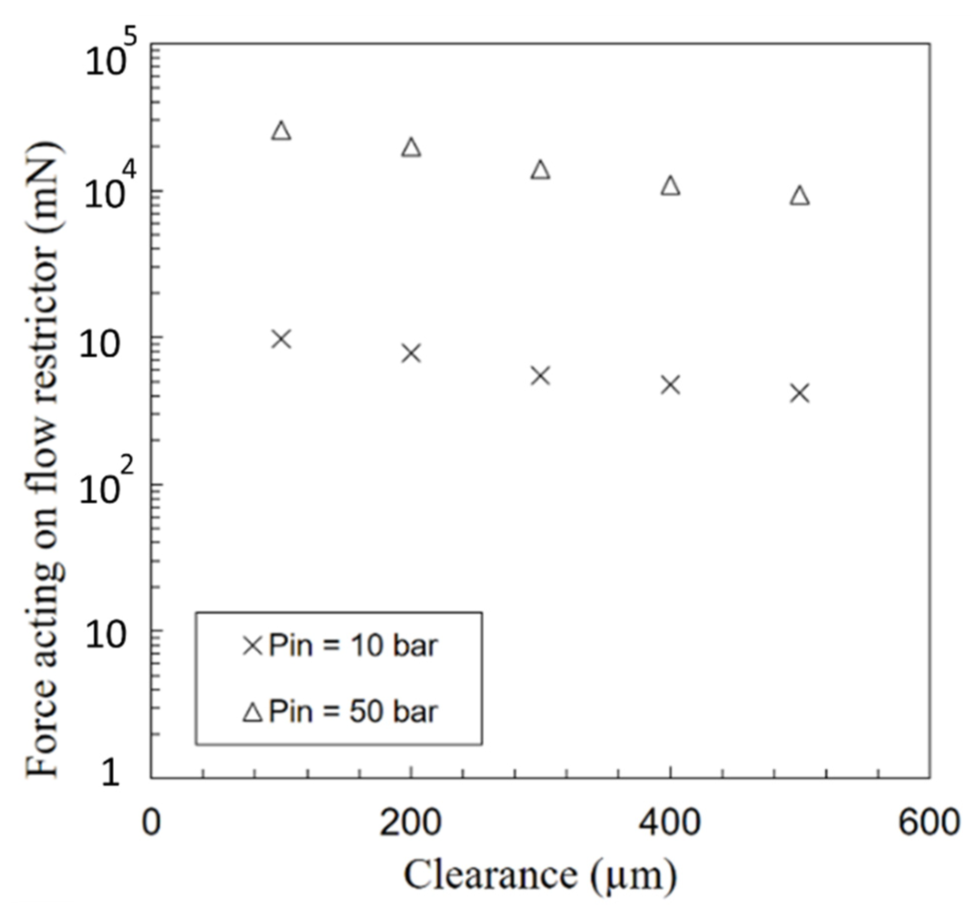
4.1. Experimental Force Analysis

Figure 3 shows the effect of clearance on the applied force on the flow restrictor. It can be seen that the force exerted on the needle shrinks with the clearance between the orifice and conical needle restrictor. However, the force exerted on the needle does not have any drastic change. Thus, it can be deduced that the conical draft angle of 15º preserves the effect of flow for high clearances and provides a stable force over the restrictor as well. A weak dependence of the force on the orifice–needle clearance exists for pressures 10 to 50 bar. This is not far from expectations, since as the clearance increases, a flow with lower velocity is blown over the needle. On the other hand, the supplied pressure has a significant effect on the exerted force. As seen in Figure 3, a five-fold increase in the supplied pressure results in an about 2500% increase in the applied force. This increase is mainly due to the sudden drop in the pressure along the needle, especially at the initial portions of the needle. Based on the numerical results, when the supplied pressure is 10 bar, approximately 60% of the pressure drop occurs at the half over the needle, while more than 80% of the pressure drop occurs at the same length for the supplied pressure of 50 bar.

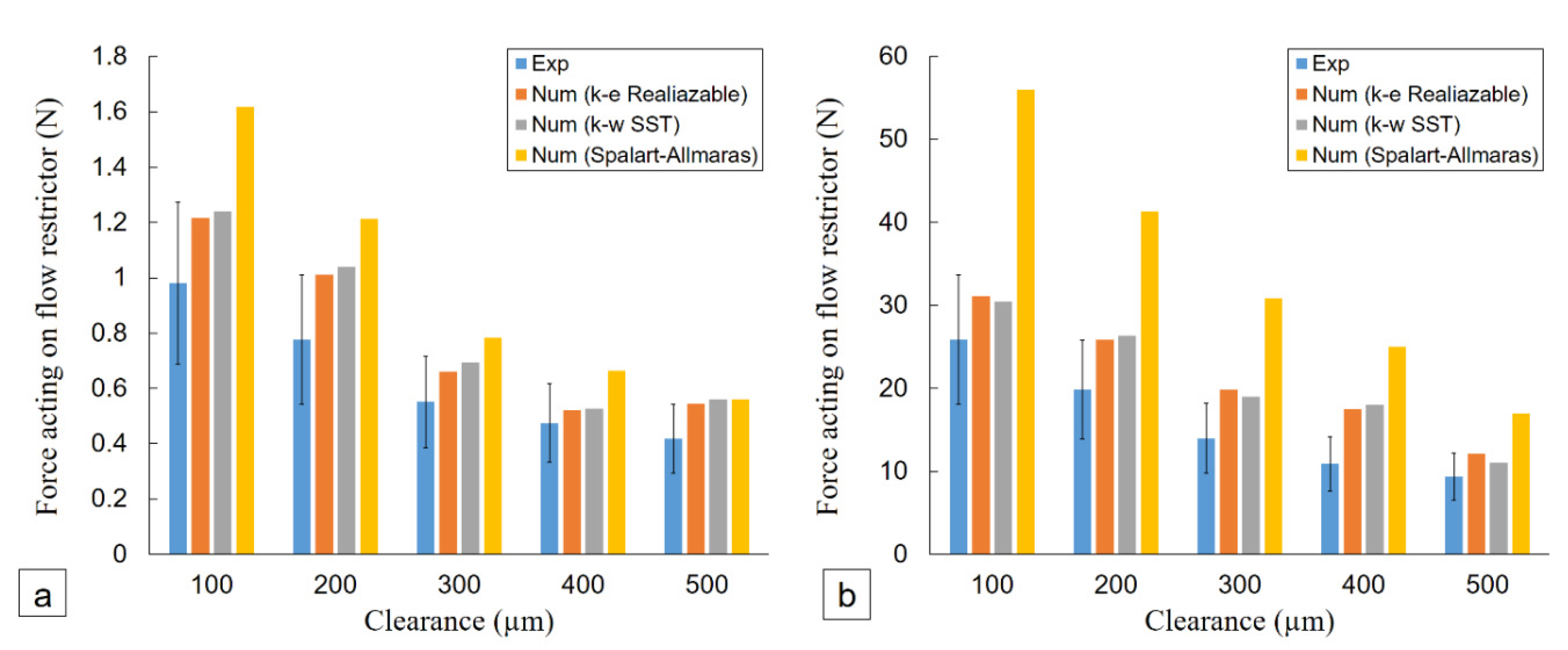
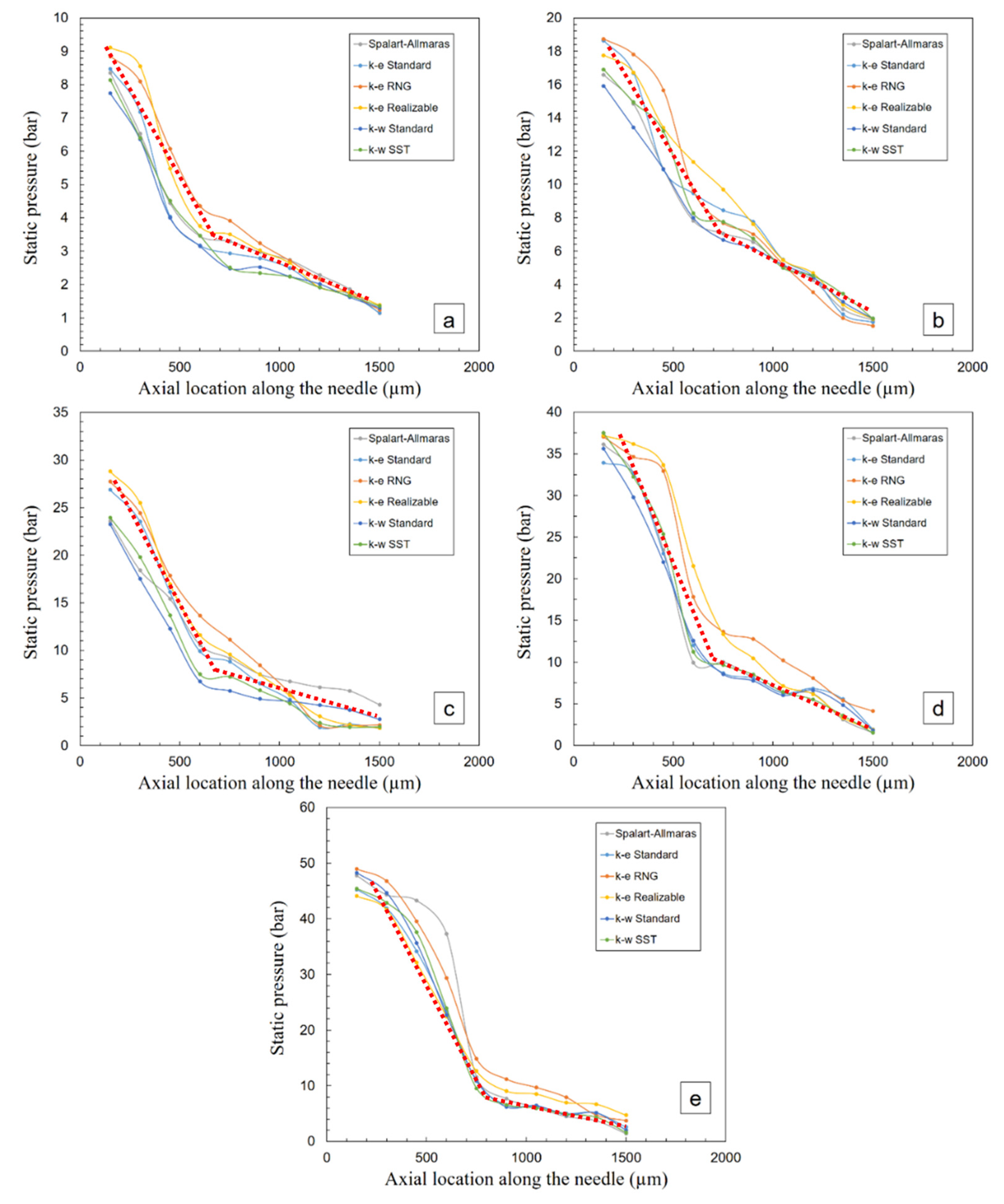
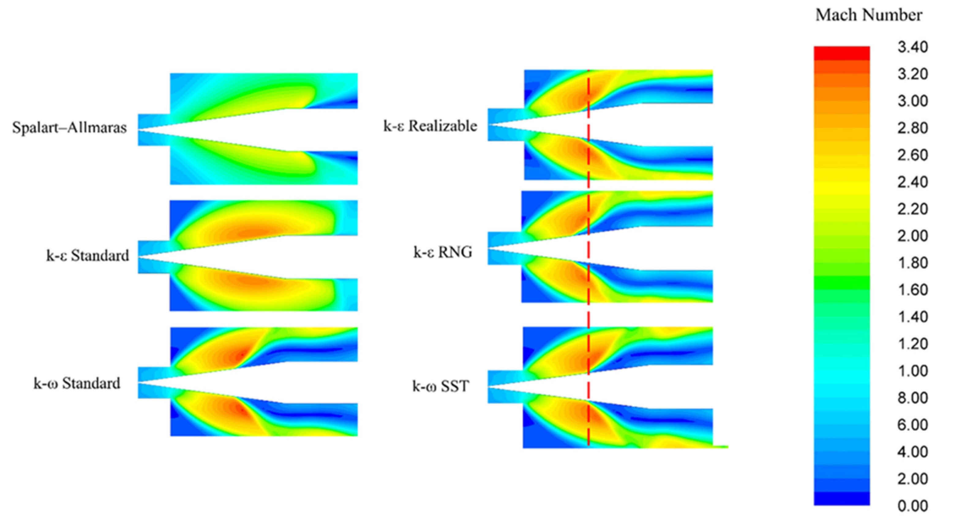
4.2. Turbulence Model Analysis

The RANS equations include Reynolds stress terms. These equations can be considered as closed equations because of the existence of more unknowns than equations. The required extra equations are provided by a turbulence closure model [38]. It should be noted that the turbulence models are sensitive at locations near stationary walls so the use of different approaches has a significant effect near these boundaries.

However, these approaches are only accurate for a certain density of meshes, where the y-plus falls within certain values. Y-plus, ($y^{+}=\frac{y{u}_r}{\upsilon }$), is a dimensionless wall distance, which depends on the distance from the nearest wall (y), friction velocity at the nearest wall (ur), and local kinematic viscosity in the turbulent flow (v). It is reasonable to apply a near-wall treatment, which does not depend on the y-plus value.

A near-wall treatment is implemented in the k–ω SST model, which lies between a viscous sublayer model (where the value of y+ is relatively small) and wall functions at y+ values (where the viscose sublayer model is not valid) [39]. Considering enhanced wall treatment for k–ε turbulence models, it can be seen that such models include a variation in near-wall treatment. Moreover, when using these k–ε turbulence models, an enhanced wall treatment model becomes available. The lack of any restriction on refining of the meshes near the wall and permission to use the same turbulence model in scaling up digesters, where obtaining small values of y-plus becomes difficult, make the mentioned model even more attractive.

Figure 4 shows the comparison in calculated forces on the bottom of the needle using the numerical model and the experimental force values for the needle with the attack angle of 15°. Comparing our numerical and experimental results, it can be seen that all the used turbulent models can be used for the prediction of the applied force on the needle, while the range of the errors lies within an acceptable span. When the externally applied pressure at the inlet is 50 bar, the Spalart–Allmaras model has the maximum relative error (equal to 60%). Generally, the k–ε realizable and k–ω SST models exhibit better performances with respect to the other applied models in this study. The maximum error of the standard form of the k–ω model is 25%.

It is worthwhile to note that although the CFD models are able to correctly determine the force induced by high-pressure gas flow, it does not necessarily predict the local phenomena in the flow. Considering the fact that each of the RANS models has been developed for specific tests, particular cases and flow phenomena, the prediction of the features of the flow should be verified at different locations for each case [40]. Therefore, a comparison regarding the locally measured values is presented for each turbulence model (static pressure of the flow along the needle). According to the obtained results shown in Figure 5, all the applied turbulence models can predict the trends in the variations of the static pressure applied on the walls of the needle. Considerable differences in obtained wall static pressures (for higher inlet pressures and specially at locations near the inlet) with the use of different turbulence models highlights the critical role of operating conditions such as flow conditions in the prediction of a different model (convergence problems as well).

The Spalart–Allmaras model with rather lower costs of computations ends up with a gratifying achievement of the results, particularly when the inlet pressures are low. It can be observed in this study that the mentioned model overpredicts the pressure prior to the shockwave relative to the experimental values. At high inlet pressures, the use of the standard form of the k–ε model results in the prediction of a normal shockwave near the end of the housing (Figure 2b). Furthermore, the use of this model ends up with the prediction of static pressure increase at the inlet of the clearance area. The results obtained from the k–ω standard model are similar to the k–ω SST model. The k–ε realizable and k–ε RNG models have similar performances. Compared with the experimental results, these models usually predict the shockwave at a more upstream position.

As mentioned before, regardless of the turbulence model, which is applied in numerical simulations, all the models predict a sudden decrease in pressure at the first half of the needle. It should be noted that at supplied pressures of 10 bar, 40 bar, and 50 bar, the pressure drop over the mentioned length is approximately 60%, 75%, and 80%, respectively. Moreover, as displayed in Figure 5, at each pressure, the pressure drop can be predicted by two different linear approximations.

Figure 6 shows the Mach number contours obtained from different turbulence models. It can be seen that the patterns of the flow have a supersonic jet entering the space between the needle tip and orifice outlet, and the flow after the shock wave is subsonic for all cases. As can be seen, compared with the other applied models, the Spalart–Allmaras model cannot be used for prediction of the shockwave location. Furthermore, the standard form of the k–ε model is unable to calculate the flow break-up, which has a considerable effect on the force analysis. Moreover, it can be inferred from comparison in the flow patterns that the most obvious difference in the applied turbulent models is the prediction of the shockwave position. Comparing the k–ε RNG and k–ε realizable models with other models, it can be observed that prediction of the shockwave obtained from these two models is at a more upstream position. The red line shows the location of the break-up point on the surface of the needle. As seen, the k–ω SST model prediction of the breakup point is more downstream on the needle surface.

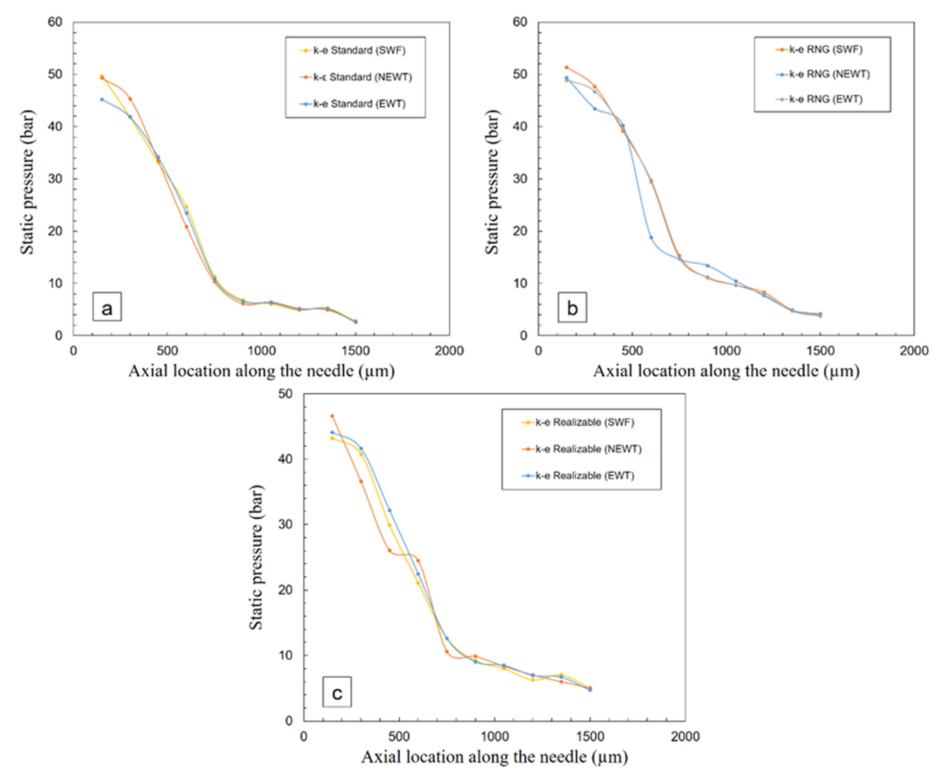
4.3. Effect of Wall Treatment

To have a better understanding of how the near-wall treatment affects the numerical results, a sensitivity analysis is conducted. Before discussing the calculated results, it is worthwhile to note the following remarks: (a) the Standard model of k–ε, k–ε RNG, and realizable configuration of k–ε models need a wall-function approach (SWF, NEWF, EWF); (b) the Standard k–ω, k–ω SST, and Spalart–Allmaras models do not require the wall function approach; (c) low-Reynolds correction is used for the standard k–ω and k–ω SST models; and (d) since the Spalart–Allmaras is used for low Reynolds numbers, it does not require any wall treatment approach.

Figure 7 shows the results corresponding to the sensitivity of the near-wall treatment where the exerted pressure at the inlet is 50 bar. Obviously, the use of different methods for the wall treatment results in differences in numerical predictions. Accordingly, it can be seen that implementation of the NEWF method instead of SWF has considerable effects, especially near the middle of the needle. The results obtained from the standard model of applying the k–ε with NEWF have less error compared with the use of the SWF for the case of calculating the applied force on the needle. The predictions of the k–ε realizable model with NEWF for the applied force are similar to those obtained with SWF. It should be noted that the use of NEWF in the k–ε RNG model leads to the residuals of more than 10⁻³. Therefore, it is not considered for further analysis. Although the obtained results from the SWF and EWT approaches do not differ considerably in most of the studied cases, the EWT approach generally achieves better results (especially for k–ε models).

As stated before, due to the low Reynold formulation of the Spalart–Allmaras model, this model does not need any wall treatment. Therefore, it provides benefits in terms of refinement of near-wall meshes. Furthermore, while using the k–ω SST model, Low-Reynolds correction does not lead to the improvement in the results for different mesh sizes used in the domain. Besides, since the k–ω SST model is independent from the wall treatment for a wider range of y-plus (y-plus < 40), this model has an advantage among the other used models in this study.

5. Conclusions

This study investigates the effect of nozzle\needle distance (clearance) and supplied pressure on micro-scale compressible flows and includes both numerical and experimental approaches. The major conclusions drawn from this study are as follows:

(i).

The exerted force on the needle shows a dramatic increase with the supplied pressure, while the exerted force decreases with the distance. Moreover, the cone angle of 15° provides a stable force for supplied pressures between 10 bar to 50 bar.

(ii).

According to the numerical results, the use of different turbulence models significantly affects the predicted results. While standard k–ε and Spalart-Allmaras models are not promising for predicting gas flow characteristics, the k–ε realizable model exhibits the best performance in predicting the results.

(iii).

Wall treatment studies reveal that the near-wall-treatment model has a considerable effect on the numerical predictions. Furthermore, the NEWF approach exhibits the worst performance among the other wall treatment approaches.

References

1. Joule, J.P.; Thomson, W. LXXVI. On the thermal effects experienced by air in rushing through small apertures. Lond. Edinb. Dublin Philos. Mag. J. Sci. 1852, 4, 481–492. [Google Scholar] [CrossRef]
2. Maytal, B.-Z.; Pfotenhauer, J.M. Miniature Joule-Thomson Cryocooling: Principles and Practice; Springer: Berlin/Heidelberg, Germany, 2012. [Google Scholar]
3. Damle, R.; Atrey, M. The cool-down behaviour of a miniature Joule–Thomson (J–T) cryocooler with distributed J–T effect and finite reservoir capacity. Cryogenics 2015, 71, 47–54. [Google Scholar] [CrossRef]
4. Ng, K.; Xue, H.; Wang, J. Experimental and numerical study on a miniature Joule–Thomson cooler for steady-state characteristics. Int. J. Heat Mass Transf. 2002, 45, 609–618. [Google Scholar] [CrossRef]
5. Liu, Y.; Liu, L.; Liang, L.; Liu, X.; Li, J. Thermodynamic optimization of the recuperative heat exchanger for Joule–Thomson cryocoolers using response surface methodology. Int. J. Refrig. 2015, 60, 155–165. [Google Scholar] [CrossRef]
6. Chen, H.; Liu, Q.-S.; Liu, Y.-W.; Gao, B. Optimal design of a novel non-isometric helically coiled recuperator for Joule–Thomson cryocoolers. Appl. Therm. Eng. 2020, 167, 114763. [Google Scholar] [CrossRef]
7. Hong, Y.-J.; Park, S.-J.; Kim, H.-B.; Choi, Y.-D. The cool-down characteristics of a miniature Joule–Thomson refrigerator. Cryogenics 2006, 46, 391–395. [Google Scholar] [CrossRef]
8. Ardhapurkar, P.; Atrey, M. Performance optimization of a miniature Joule–Thomson cryocooler using numerical model. Cryogenics 2014, 63, 94–101. [Google Scholar] [CrossRef]
9. Chua, H.T.; Wang, X.; Teo, H.Y. A numerical study of the Hampson-type miniature Joule–Thomson cryocooler. Int. J. Heat Mass Transf. 2006, 49, 582–593. [Google Scholar] [CrossRef]
10. Damle, R.; Atrey, M. Transient simulation of a miniature Joule–Thomson (J–T) cryocooler with and without the distributed J–T effect. Cryogenics 2015, 65, 49–58. [Google Scholar] [CrossRef]
11. Hoxton, L.G. The Joule-Thompson effect for air at moderate temperatures and pressures. Phys. Rev. 1919, 13, 438. [Google Scholar] [CrossRef]
12. Roebuck, J. The Joule-Thomson effect in air. Proc. Am. Acad. Arts Sci. 1925, 60, 537–596. [Google Scholar] [CrossRef]
13. Roebuck, J. The Joule-Thomson effect in air. Second paper. Proc. Am. Acad. Arts Sci. 1930, 64, 287–334. [Google Scholar] [CrossRef]
14. Roebuck, J.; Osterberg, H. The Joule-Thomson effect in nitrogen. Phys. Rev. 1935, 48, 450. [Google Scholar] [CrossRef]
15. King, R.; Potter, J. An Axial-Flow Porous Plug Apparatus1. ASME Pap. 1962, 61, 1–226. [Google Scholar]
16. Pocock, G.; Wormald, C.J. Isothermal Joule–Thomson coefficient of nitrogen. J. Chem. Soc. Faraday Trans. 1 1975, 71, 705–725. [Google Scholar] [CrossRef]
17. Zelmanov, J. Joule-Thomson effect in helium at low temperatures. J. Phys. USS FI 1940, 3, 43. [Google Scholar]
18. Roebuck, J.; Osterberg, H. The Joule-Thomson effect in argon. Phys. Rev. 1934, 46, 785. [Google Scholar] [CrossRef]
19. Johnston, H.L.; Bezman, I.I.; Hood, C.B. Joule-Thomson Effects in Hydrogen at Liquid Air and at Room Temperatures1. J. Am. Chem. Soc. 1946, 68, 2367–2373. [Google Scholar] [CrossRef]
20. Gladun, A. The Joule-Thomson effect in neon. Cryogenics 1966, 6, 31–33. [Google Scholar] [CrossRef]
21. Koeppe, W. On the Joule−Thomson Effect of Gases and Mixtures. Kaltetechnik 1959, 11, 363–369. [Google Scholar]
22. Hartmann, H.; Mann, R.; Neumann, A. Ein Beitrag zum Joule–Thomson–Effekt von Stickstoff-Wasserstoff-Gemischen. Ber. Bunsenges. Phys. Chem. 1969, 73, 492–497. [Google Scholar]
23. Sreedhar, R.; Sreedhar, A. Joule–Thomson cooling with binary mixtures. Infrared Phys. Technol. 1998, 39, 451–455. [Google Scholar] [CrossRef]
24. Roebuck, J.; Osterberg, H. The Joule-Thomson Effect in Mixtures of Helium and Argon. J. Chem. Phys. 1940, 8, 627–635. [Google Scholar] [CrossRef]
25. Little, W. Microminiature refrigeration. AIP Conf. Proc. 2008, 985, 597–605. [Google Scholar]
26. Little, W.A. Fast Cooldown Miniature Refrigerators. U.S. Patent No. 4,489,570, 25 December 1984. [Google Scholar]
27. Shapiro, A.; Fraiman, L.; Parahovnik, A. Ceramic 3D printed Joule Thomson mini cryocooler intended for HOT IR detectors. In Tri-Technology Device Refrigeration (TTDR) II; SPIE: Bellingham, WA, USA, 2017; Volume 10180, pp. 48–60. [Google Scholar]
28. Sadaghiani, A.K.; Koşar, A. Numerical and experimental investigation on the effects of diameter and length on high mass flux subcooled flow boiling in horizontal microtubes. Int. J. Heat Mass Transf. 2016, 92, 824–837. [Google Scholar] [CrossRef]
29. Aboubakri, A.; Akkus, Y.; Sadaghiani, A.K.; Sefiane, K.; Koşar, A. Computational and experimental investigations on the evaporation of single and multiple elongated droplets. Chem. Eng. J. Adv. 2022, 10, 100255. [Google Scholar] [CrossRef]
30. Xie, Z.; Wang, X.; Zhu, W. Theoretical and experimental exploration into the fluid structure coupling dynamic behaviors towards water-lubricated bearing with axial asymmetric grooves. Mech. Syst. Signal Process. 2022, 168, 108624. [Google Scholar] [CrossRef]
31. Lin, Q.; Wei, Z.; Wang, N.; Chen, W. Analysis on the lubrication performances of journal bearing system using computational fluid dynamics and fluid–structure interaction considering thermal influence and cavitation. Tribol. Int. 2013, 64, 8–15. [Google Scholar] [CrossRef]
32. Liang, Y.; Yang, Y.; Shan, X.; Wang, Z. Effect of Airfoil Dimple on Low-Reynolds-Number Differing Laminar Separation Behavior via Multi-Objective Optimization. J. Aircr. 2022, 9, 1–14. [Google Scholar] [CrossRef]
33. Dong, C.; Cui, X.; Liu, S.; Jiang, Z.; Wu, Y. Investigation on the choked mass-flow characteristics of the helium fluid during the Joule-Thomson process in micro-orifice under different high pressures. Cryogenics 2022, 122, 103416. [Google Scholar] [CrossRef]
34. Baki, M.; Okutucu-Özyurt, T.; Sert, C. Optimization of Joule-Thomson cryocooler heat exchanger using one-dimensional numerical modeling. Cryogenics 2019, 104, 102981. [Google Scholar] [CrossRef]
35. Lemmon, E.W.; Huber, M.L.; McLinden, M.O. NIST reference fluid thermodynamic and transport properties–REFPROP. NIST Stand. Ref. Database 2002, 23, v7. [Google Scholar]
36. Poling, B.E.; Prausnitz, J.M.; O’Connell, J.P. The Properties of Gases and Liquids; Mcgraw-Hill: New York, NY, USA, 2001; Volume 5. [Google Scholar]
37. Fluent, A. Ansys Fluent Theory Guide; ANSYS Inc., USA: Canonsburg, PA, USA, 2011. [Google Scholar]
38. Menter, F.R. Turbulence Modeling for Engineering Flows; Technical Paper; ANSYS Inc., USA: Cannonsburg, PA, USA, 2011; pp. 1–25. [Google Scholar]
39. Menter, F.; Kuntz, M.; Langtry, R. Ten years of industrial experience with the SST turbulence model. Turbul. Heat Mass Transf. 2003, 4, 625–632. [Google Scholar]
40. Wilcox, D.C. Turbulence Modeling for CFD; DCW Industries: La Canada, CA, USA, 1998; Volume 2. [Google Scholar]
Figure 1. (a) Experimental setup and components: (b) test section; and (c) needle geometrical characteristics.
Fluids 07 00151 g001
Figure 2. (a) Computational domain; (b) needle and housing configuration; and (c) needle draft angle.
Fluids 07 00151 g002
Figure 3. Obtained experimental results of exerted forces for the needle draft angle of 15° at upstream pressures of 10 and 50 bar.
Fluids 07 00151 g003
Figure 4. Numerical and experimental results of force analysis for needle draft angle of 15° at (a) inlet pressure of 10 bar and (b) inlet pressure of 50 bar.
Fluids 07 00151 g004
Figure 5. Calculated wall static pressures along the needle inside the orifice with a clearance of 300 µm at different upstream pressures of: (a) 10 bar; (b) 20 bar; (c) 30 bar; (d) 40 bar; and (e) 50 bar.
Fluids 07 00151 g005
Figure 6. Mach number contours for ejected flows from the micro nozzle for different turbulence models.
Fluids 07 00151 g006
Figure 7. The effect of wall treatment on wall static pressure at the inlet pressure of 50 bar for tip clearance of 200 µm for (a) Standard k–ε model, (b) k–ε RNG model, and (c) k–ε Realizable model.
Fluids 07 00151 g007