Article

Coexistence of Inverse and Direct Energy Cascades in Faraday Waves

1
Institute of Multiphase Flows, Hamburg University of Technology, 21073 Hamburg, Germany
2
Department of Mechanical Engineering and Production, Hamburg University of Applied Sciences, 20099 Hamburg, Germany
*
Author to whom correspondence should be addressed.
Fluids 2022, 7(5), 148; https://doi.org/10.3390/fluids7050148
Submission received: 14 February 2022 / Revised: 10 April 2022 / Accepted: 19 April 2022 / Published: 24 April 2022
(This article belongs to the Section Turbulence)

Abstract

:
In nature, turbulent flows exist that are neither simply 2D nor 3D but are forced towards one state or the other by boundary conditions such as varying stratification. Here, we report the first evidence of the co-existence of an inverse and a direct energy cascade in an experimental flow driven by Faraday waves in water. We find that an inverse energy cascade at the fluid surface and a direct energy cascade in the 3D bulk flow underneath co-exist. We base our analysis on temporally and spatially well-resolved velocity fields obtained by particle image velocimetry measurements at planes parallel and perpendicular to the water surface. The findings also provide strong evidence that the intense turbulent 2D surface flow drives the 3D bulk flow through sporadic vertical jets as a source of momentum to the bulk liquid.
PACS:
47.27.-i; 47.80.Cb; 47.80.Jk

1. Introduction

The study of two-dimensional three-component (2D3C) flows has placed particular emphasis on the occurrence of an inverse energy cascade in thick layers and the transition from 2D to 3D turbulence and vice versa [1,2]. Examples of experimental flows exhibiting an inverse cascade, as expected for 2D turbulence, are electromagnetically driven (EMD) flows [3] and flows occurring on the surface of parametrically excited waves [4,5,6]. These Faraday waves [7] have become a test-bed for the study of 2D-turbulence since the discovery of a horizontal surface flow, termed Faraday flow [4,8,9]. However, early experiments were conducted in thin-layer systems, where the fluid depth is negligible compared to the characteristic length of the flow structures which are of approximately the size of the Faraday wavelength λ F . Recently, experiments at the fluid surface and at submerged planes in a non-shallow Faraday system characterized the sub-surface velocity fields [10]. The study unveiled the previously unknown existence of 3D bulk flows with a rich variety of complex flow structures. An exponential decay in the mean velocity magnitude and in mean vorticity with depth was observed, proving the confinement of the strong 2D turbulence to the fluid surface, as suggested by other theoretical and experimental work on wave-induced flows [5,11,12,13]. The study [10] identified three regimes, namely the 2D Faraday flow at the surface, a transition regime of decay in velocity and vorticity right below the surface, and a bulk flow regime where large and slow three-dimensional structures are dominant. However, the mechanism of energy injection and energy transport through scales remained unclear: how are the surface and the bulk flow related in terms of energy and momentum transfer? What is the mechanism that fuels the fluid motion beneath the surface? Is an inverse energy cascade or at least a remnant of it also observed in the fluid bulk as was observed for a thick-layer EMD-driven flow [14]?
This study answers the above questions and reports the co-existence of an inverse energy cascade, localized at the fluid surface, and a direct energy cascade in the 3D bulk flow underneath in an experimental flow. Furthermore, sporadic vertical jets, which drive the vertical transport of energy and momentum from the surface to the bulk flow are found in experimentally derived velocity fields.

2. Materials and Methods

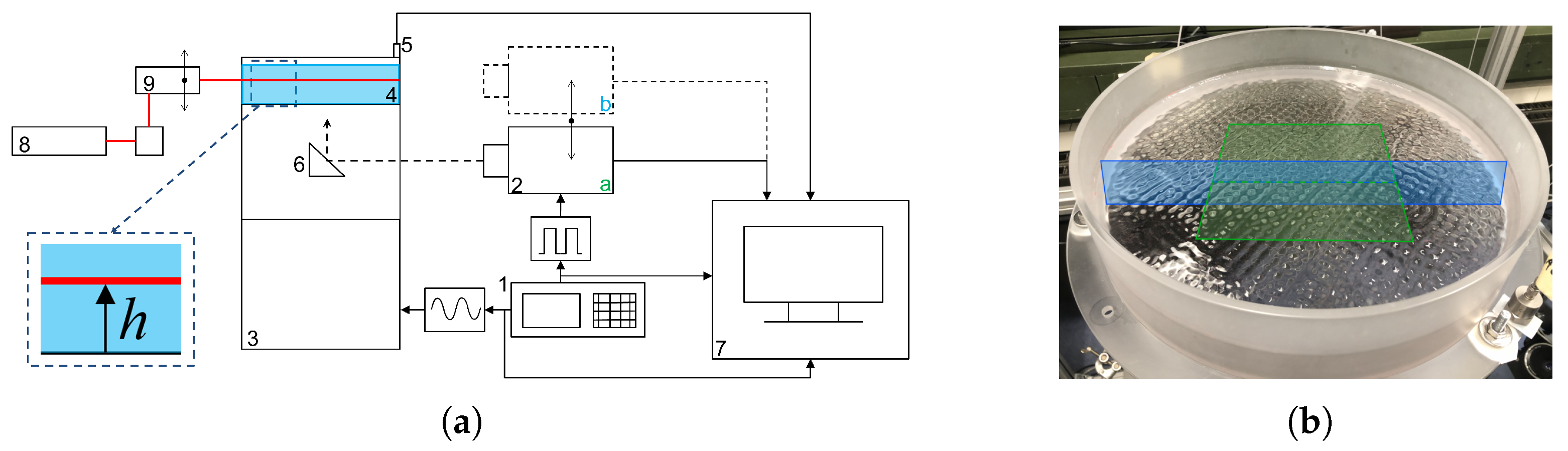
2.1. Experimental Setup

The Faraday experiment was recreated with the experimental setup previously described in [10], and is presented in Figure 1 for both the horizontal (parallel to the surface) and vertical (perpendicular to the surface) PIV measurements. A function generator (1, RIGOL) and an electromagnetic shaker (3, TIRA TV5220) were used to vertically oscillate a cylindrical container of 290 mm diameter (4) with a monochromatic sinusoidal signal at the forcing frequency f f = 50 Hz. The container was filled with a 30 mm-thick layer of distilled water. The Faraday waves, which appeared as quasi-standing waves on the fluid surface (see Figure 1b), showed a subharmonic response to the external forcing at f F = 25 Hz. At this frequency, the characteristic wavelength of the Faraday waves is ( λ F = 9.5 ± 1.0 ) mm. The amplitude of the forcing acceleration a f was measured by two accelerometers attached on the container (Kistler, ± 5 g, sensitivity 1 g/V ± 10 % ) and set to a f = 0.47 g and a f = 0.70 g, respectively, consistent with the values in [10]. At lower forcings than a f = 0.47 g, the Faraday flow on the liquid surface appeared still very ordered and not fully turbulent. Furthermore, from about this forcing intensity upwards, vertical jets were observed below the surface. The upper bound of the forcing amplitude, a f = 0.70 g, was set due to increasingly disturbing reflections on the liquid surface which impaired the quality of the PIV analysis. The changes in the observed flow behavior in between these two forcing frequencies were only gradual. PIV measurements were performed using red fluorescent polyethylene microspheres of diameter 10–45 µm (Cospheric) as flow tracer. The particles have a density of 0.995 g/cm3 and uniformly disperse in the water volume. For that, 0.3 g of particles are wetted in a 10%-solids solution with a surfactant (1% Tween 80 solution, Polysorbate 80, non-ionic). No effects of buoyancy were observed; inertial effects are negligible and particles can be considered as perfect fluid tracers with Stokes numbers S t 10 4 [15]. Imaging was performed with a high-speed camera (2, Phantom VEO 640L, resolution: 2560 × 1600 px), which was triggered at f rec = 400 Hz by a second signal from the function generator (standard 5V TTL signal). This allowed us to carefully synchronize the phase delay between the Faraday wave forcing and the imaging and thus to capture the flat surface of the waves two times (every eighth frame) per full wave period T F (corresponds to 16 frames). Furthermore, it helps to synchronize the imaging such that frame i and frames i + n · 8 , n N are taken at the same container height. For the horizontal plane measurements, the camera is positioned below the container (2a) and an optical mirror is used to deflect the camera’s line of sight in the vertical direction. The tracer particles are illuminated by a continuous wave argon-ion laser (8, wavelength of 488 nm, Ion Technologies), which is expanded to a planar laser sheet (2 mm thick, 80–100 mm wide) with a set of laser optics (9). From the forcing acceleration, the computed maximum container displacement of ( 7.10 ± 0.71 ) · 10 3 mm was found to be sufficiently small in comparison to the laser sheet thickness such that it has a negligible effect onto the velocity fields and no correction for this external movement needs to be considered. PIV measurements were carried out at four horizontal planes at a distance h from the container bottom, h = 30, 27, 21 and 4 mm. These heights were chosen due to previously published results [10], wherein three distinct flow regimes at different heights were observed. The measurement height h = 21 mm was additionally selected because by observing the flow, we determined that this was the approximate height where vertical jets that rushed down from the surface would often disperse. The horizontal PIV measurements at the fluid surface were performed with LED light to prevent reflections of the laser sheet at the wave–air interface. For the vertical PIV measurements, the laser sheet was tilted by 90° in order to vertically cut through the flow domain to obtain temporally and spatially well-resolved velocity information in the vertical cross-section of the container.
The high-speed camera is placed in this case at the container level (2b), looking directly through the container side. For each forcing acceleration, six statistically independent measurement runs were carried out on the horizontal surface plane and four statistically independent measurement runs on all other vertical and perpendicular planes each.

2.2. PIV Processing

For an optimal PIV, processing a careful calibration is indispensable, especially in the case of vertical recordings since particle image distortions due to the bent acrylic container walls are massive. To determine the local conversion between spatial distance (in mm) and pixel distance (in px) and correct for the distortion in each recorded image, calibration images were captured on the same plane for each measurement. For this purpose, a two-level double-sided calibration plate with a white precision dot-pattern on black ground was used (type 058-5, dot-spacing 5 mm, LaVision GmbH). The resulting calibration coefficients allowed to correct the distortion (dewarping) of all particle images using the perspective correction function of the DAVIS 10.1.2 Software (LaVision GmbH) prior to PIV processing. As the distance between the camera objective and focus plane differed in each measurement, the conversion was not constant as summarized in the Appendix A. Subsequently, the velocity fields were obtained from the corrected particle images with the PIV analysis software PIVview 3.8.0 (PIVTEC GmbH). The PIV parameters and the used algorithm are summarized in the Appendix A and Appendix B. A particle displacement of 4–10 pixels per image pair is desirable. However, the flow velocities decrease rapidly away from the fluid surface towards the container bottom and there is a large dynamic range of particle displacements between consecutive images. Using the PIV analysis with a single inter frame time Δ t would yield either an underestimation of the slow velocities at the container bottom or a complete loss of correlation close to the liquid surface. Therefore, each recorded image is subdivided into three slightly overlapping vertical domains (one velocity grid element overlap). For each vertical domain, a different inter-frame time Δ t is chosen in order to optimize the PIV analysis. Δ t is thereby always a multiple of the recording inter-frame time Δ t = n · t rec , t rec = 1 / f rec such that an optimal analysis of the resulting velocity fields on each height can be assured. The values of the inter-frame times used for PIV-analysis are summarized in the Appendix A and Appendix B together with a sketch of the subdivision of the image domains (see also Supplementary Figure S2). The full velocity field is reconstructed by merging the three domains with interpolation at the interfaces. The start and end values of the vertical domains in the vertical direction are h [ 1.68 , 14.34 ] mm for the lower one, h [ 14.34 , 21.37 ] mm for the middle section and h [ 21.37 , 28.06 ] mm for the upper domain. Due to the container acting as a converging lens and reflections at the surface, some information of the vertical recorded images is lost, such that only heights between h = 1.68 mm and h = 28.06 mm can be analyzed. The evaluation of the horizontal measurements is conducted as previously explained [10]. Here, we present measurements planes at h = 30, 27, 21 and 4 mm.

2.3. Spectral Analysis of Velocity Fields

To analyze the turbulence at the surface and various submerged planes below it, we calculated the energy and the enstrophy spectra in the frequency domain. Beforehand, to reduce the spurious residual from the rectangular camera image, we used a Tukey windowing function to smoothen the spatial velocity and vorticity fields at the edges and zero-padding. The 2D energy and enstrophy spectra were subsequently averaged over all discrete time steps to the improve statistical significance. Instantaneous and time-averaged spectra were found to yield similar results which suggests statistical convergence. The direction-independent energy spectra E ( | k | ) were obtained by the ring binning of the 2D energy spectral fields [16]. To determine the inter-scale spectral flux through particular wavelengths λ n , n N , a spatial filter of varying width [17,18] originally used for large-eddy-simulations (LES) [19,20,21] was applied on the velocity fields. Low-pass filtering was obtained by a smooth fourth-order Butterworth filter acting on each dimension separately in the frequency domain. The energy flux Π E λ n = τ i j ˜ s i j ˜ , i , j [ 1 , 2 ] was calculated from the 2D data as described in [22], with s i j ˜ = 1 2 u ˜ i x j + u ˜ j x j being the strain rate of the filtered velocity fields and τ i j ˜ = u i u j ˜ u ˜ i u ˜ j the turbulent stress tensor. Analogously, an expression for the enstrophy flux based on the vorticity ω can be found [18]:
Π E λ n = u i u j ˜ u ˜ i u ˜ j u ˜ i x j
Π Z λ n = u i ω ˜ u ˜ i ω ˜ ω ˜ x i
A negative spectral flux Π λ n < 0 implies net energy transport towards smaller scales while a positive spectral flux Π λ n > 0 implies net energy transport towards larger scales.

3. Results and Discussion

In this study, velocity measurements in the vertical plane enhance the understanding on the mechanisms of energy transport between the two-dimensional Faraday flows confined to the fluid surface, and the intrinsically 3D flow that is observed underneath. For the following figures and diagrams, the velocity components in the three spatial directions are denoted as u = u , v , w . Figure 2 depicts examples of instantaneous velocity fields in the vertical planes for a f = 0.47 g (a) and a f = 0.70 g (b), highlighting the presence of strong vertical jets (see red arrows) that cause a locally intense downward transport of fluid from the surface to the bulk. For both forcing accelerations, the jets typically dissolve at approximately one Faraday wavelength below the surface (9–10 mm). These jets are also observed in the horizontal velocity fields at the corresponding plane ( h = 21 mm) as fluid and momentum sources, i.e., positive divergence, with velocity arrows pointing outwards from a central point, as can be seen in Figure 3c and Supplementary Figure S4c. The jets occur sporadically and the estimated occurrence frequency is in the range of 0.5 up to a few Hz. Therefore, it is not always possible to find two jets in one instantaneous velocity field. From the divergence fields of the surface flow, a rough estimate of the jet-to-jet distance is d j e t , approximately 5 to 10 λ F while the average life-time of a jet (the time while a direct downward flow from the surface occurs) is in the range of τ j e t 40 T F , where T F is the Faraday wave period. Because of the localized high velocity and strong vertical fluid transport, it is very reasonable to assume that these jets drive the flow structures below the surface and act as an energy-injecting mechanism for the 3D bulk flow. Concurrently, their formation causes the generation of vortices on both sides of the jets with the vorticity pointing parallel to the liquid surface. In Figure 4, the sub-surface profiles of the mean absolute velocities in dependence of the measurement height for both forcing accelerations, a f = 0.47 g and a f = 0.70 g, are depicted. The mean absolute velocities | u | , | v | , | w | were calculated by averaging the absolute velocity over time and all measurement runs for each fluid height. For the horizontal measurements, the components | u | and | v | can be calculated and for the vertical measurements | u | and | w | .The values of | u | and | v | from the horizontal measurements should thereby coincide with the vertical measurements of | u | at the same height. The data from the vertical and the horizontal measurements agree well. Both diagrams combine the vertical and horizontal PIV measurements for one forcing amplitude. The data are also compared with the data published in [10] in Supplementary Figure S3.
In order to further study the energy content in the bulk flow, the average ratio of flow kinetic energy in the vertical direction to the total flow kinetic energy is computed from the vertical PIV measurements: E kin , z / E kin , tot = w 2 / u 2 + v 2 + w 2 w 2 / u 2 + u 2 + w 2 . Thereby we assume that u 2 v 2 is valid on a statistical average over time and space, as also verified by the very similar profiles of | u | and | v | in Figure 4. The average ratio of the flow kinetic energy profile along the height h is depicted in Figure 5. The vertical component of the kinetic energy gradually increases to peak in a layer of approximately one Faraday wavelength below the surface. In this layer, the energy content in the z-direction becomes dominant (larger than 1/3). This can be explained by the presence of the confined and strong downwards jets seen in the velocity fields (Figure 2). At lower depths, for h < 20 mm, the influence of w 2 gradually decreases and becomes negligibly small close to the container bottom (around 5%). In summary, the energy content below Faraday waves is dominated by horizontal flow components but a local peak emerges where the vertical motion caused by intense jets becomes dominant.
From the analysis of velocity structures and kinetic energy profiles, four horizontal x-y planes were selected for the measurements of horizontal velocity fields and flow structures, located at depths of h = 4 , 21, 27 and 30 mm. The results for a f = 0.47 g are presented in Figure 3 while the results of a F = 0.70 g can be found in Supplementary Figure S4. To visualize the movement of the tracer particles, the raw images were averaged over a given time span Δ t , which varies depending on the local flow velocity and particle displacement. The images depict a sub-region of the whole measurement window with the dimensions 80 × 80 mm2, which is approximately one third of the entire field of view. An enlargement section of 25 × 25 mm2 additionally shows the corresponding instantaneous velocity fields. For comparison, the Faraday wavelength λ F = ( 9.5 ± 1.0 ) mm (approximately corresponding to twice the energy injection length scale) is depicted. The observations and conclusions apply for both accelerations a f as the same characteristic structures appear in the velocity field for both cases. Three distinct flow regimes at different heights can be identified from the horizontal planar measurements. On the fluid surface, the main features of the significantly turbulent Faraday flow can be identified by the presence of multiple vortices, with a typical size varying between 1/2 and 2 Faraday wavelengths, and rapid bursts of horizontal jet-like flow accelerated between them. The Reynolds number (based on half the Faraday wavelength and average absolute velocity of one component | u | varies in this regime between 21 for the lower forcing and 41 for a f = 0.70 g. This highly turbulent flow, with short time scales, is exclusively confined in a thin layer of the fluid surface (approximately 2 mm thick), with vorticity vectors pointing perpendicular to the fluid surface and velocity components in the horizontal plane. A second “transition" regime was identified for h between 20 and 28 mm. In this regime, the velocity magnitude exponentially decreases before reaching the plateau presented in Figure 4. The Reynolds numbers, based on characteristic length determined from spatial correlations as shown in [10], range here between 3 and 17. Here, the flow structures become slower and less turbulent, but still carry the imprint of vortical structures of the surface flow, as well as the effects of the vertical jets. This can be seen particularly well in Figure 3c and Supplementary Figure S4c, which show the presence of positive divergence, identified by velocity vectors pointing outwards from the source point, which indicates the presence of a jet as it dissolves by impinging on the slower flow at lower depths. The third regime starts at h 20 mm right below the depth at which vertical jets typically dissolve, and extends down to the container bottom. Here, no more vortical structures are observed in the horizontal velocity fields, but instead, only slowly varying large scale motions with very long temporal scales and Reynolds numbers varying in this domain between 3 and 9. The vorticity and divergence of the horizontal velocity fields at these heights were analyzed in [10]. These large-scale motions are, however, different from the previously reported streaming effects caused by standing waves as theoretically described [23] and experimentally observed for longitudinal Faraday waves [24]. The measured structures are several Faraday wavelengths in size and excessively large to be explained by classical streaming patterns that are of the order of half the wavelength of the standing wave [23]. It is thus likely that they are also largely driven by the downward jets. In addition to the description of flow structures and kinetic energy profiles, the spectral analysis of energy transport and net energy and enstrophy fluxes through the scales was performed at the aforementioned planes. The results are depicted in Figure 6 for h = 30 , 27 and 21 mm and both forcing accelerations (note the different scales among the panels). The results for h = 4 mm are not shown.
The results in Figure 6a clearly validate the double-cascade feature of 2D turbulence in the Faraday flow on the fluid surface [4,8,9], even for the large fluid thickness of 3 cm. For both forcing accelerations, it is possible to recognize a sharp bend in the energy spectrum occurring at approximately the energy injection wavenumber k inj 2 π / ( λ F / 2 ) = 1.3 mm−1 (computed with half the Faraday wavelength as the dominant forcing scale for energy injection). At wavenumbers k < k inj , the slope of k 5 / 3 is captured fairly well, and the negative net energy flux Π E ( k ) validates the presence of an inverse energy cascade, although the transition from negative to positive is not localized at one wavenumber as in theory or simulated flows [1,25] but occurs more gradually. Our data also resolve the direct enstrophy cascade with a positive net enstrophy flux Π Z ( k ) for k > k inj . The slope of E ( k ) is, however, slightly steeper than the k 3 scaling predicted by Kraichnan [26]. This phenomenon is not uncommon in experimental 2D turbulence, where friction and damping effects can cause deviations at larger wavenumbers in contrast to theory or simulated data [9,25]. The situation is substantially different in the plane immediately below the fluid surface—at h = 27 mm—shown in Figure 6b. The slope of the energy spectra is more homogeneous throughout the entire wavenumber range and no distinct bend can be seen at the energy injection wavenumber. Here, in sharp contrast to the surface flow, the net energy flux remains positive for all wavenumbers, proving that the flow exhibits a direct energy cascade and that there is a transition from the 2D turbulent Faraday flow on the surface to a direct energy cascade right below the surface. This observation is validated by the zero net enstrophy flux, indicating the vanishing influence of the direct enstrophy cascade. The results for the energy fluxes and spectra are similar at further submerged planes below the surface (e.g., h = 21 mm, Figure 6c and h = 4 mm, not shown), where both trends of positive net energy flux and zero net enstrophy cascade are confirmed, although with much smaller magnitudes than at h = 27 mm. This is also observed in the velocity fields, as the flow becomes less turbulent, and the velocity structures become larger, less chaotic and with longer temporal scales [10]. In Figure 6c, at h = 21 mm, there is a valley in the energy flux at intermediate scales ( k 7 mm−1 corresponding to 9 mm λ F ) that we cannot definitely explain. A possible interpretation is that the positive divergence (sources are of sizes λ F , see Figure 3c) caused by the impinging vertical jets caused some upscale energy transport by stretching out on that plane, diminishing the positive mean value of Π E ( k ) . This would also explain why the effect is not seen at h = 27 mm.
The results add to the findings on 2D3C flows as described in [1,2,3,5,13] by proving for the first time the co-existence of an inverse and a direct energy cascade in an experimental flow. Interestingly, early experiments on electromagnetically driven flows in thick layers rather observed the opposite, a sustained inverse cascade at submerged planes despite substantial 3D motion [14]. However, due to the different forcing principle and a maximal horizontal velocity within the EMD bulk flow, it is reasonable that the resulting flows are very different, even if they appear similar at the surface. Both fundamentally different transport mechanisms for energy and momentum clearly coexist naturally here, while in previously reported experimental flows a forward or an inverse energy cascade was achieved by switching between the different boundary conditions or modifying the physical system through stratification or applied rotation, as summarized in [1]. Furthermore, the two different cascades directly interact in close proximity to the fluid surface.
A possible pathway of the energy could therefore be described as follows: In a thin surface layer at the air/water interface, the chaotic and disordered behavior of the flow at small scales leads to the formation of larger, more ordered structures such as the vertical surface jets which are likely to correspond to the coherent bundles studied in detail in [27,28]. Energy is transferred upscale by the inverse cascade until the surface energy spectra tend to level out at wavenumbers k ≲ 0.2 mm−1 (Figure 6a,b). There, energy might be lost due to the clashing of the vertical surface jets which then cause the sporadic downward jets, thereby fueling the direct cascade found in the bulk flow below. The interpretation that energy is transferred from the surface flow to the bulk and not vice versa is also supported by the estimates of the mean energy injection rates ϵ i n that are calculated as ϵ i n = | Π E i n | = | k 1 k 2 Π E ( k ) / k 2 k 1 | , where [ k 1 , k 2 ] denotes the interval of a potential inertial range in the corresponding cascade, even though the energy flux is not constant (see Supplementary Figures S5 and S6). The approximate values for the energy injection rates ϵ i n of the direct cascades at h = 27 mm are only approximately 14 % of the energy injection rates at the fluid surface h = 30 mm, for both forcing accelerations.
In addition to the surface velocity structures, the Faraday waves might also have an impact onto the occurrence of vertical downward jets. A possible mechanism for a vertical jet to form could be the coincidence of clashing jets and downward motion due to a particularly intense wave. The disordered motion of the individual waves, called oscillons, was recently studied and its correlation to the surface flow was confirmed [5,29]. In the current study, it was not feasible to simultaneously monitor the velocity field and the surface height due to the dense seeding necessary to obtain high quality velocity fields suitable for spectral analysis. In other studies of Faraday waves, the Lagrangian trajectories of particles were recorded together with the wave field using a diffusing light imaging technique [27,28].However, seeding in these cases was much less dense and largely contained to the surface due to buoyant tracer particles. Therefore, the technique could not be used here. A possible path to obtain both the wave height and the flow simultaneously would be three-dimensional particle tracking. The trajectories of the particles would then naturally carry the information of the height and thus the wave pattern. This measurement, however, implies three-to-four high-speed cameras and is intensive in equipment. Furthermore, the difficulty of surface reflections even when fluorescent particles are used also persists herein and is especially strong for large waves and finally, the surface causes the increased occurrence of so-called ghost particles in PTV analysis.A future study should also consider the possible effect of varying surface contamination on the formation of vertical jets since it is known that this might have a considerable effect on the surface forces that induce the horizontal surface movement of the liquid [24,30,31].

4. Conclusions

In this study, we performed the analysis of energy spectra and mean spectral energy fluxes in non-shallow Faraday waves obtained from planar PIV measurements at different submerged planes and the surface. For the first time, an inverse energy cascade on the fluid surface and a co-existing direct energy cascade in the 3D bulk flow underneath were observed in an experimental flow. The double cascade regime of the Faraday flow was well captured by our experiments, clearly showing a change in the energy spectral slope at approximately the energy injection wavenumber k inj = 1.3 mm−1 and an inverse energy cascade with negative net energy flux towards larger scales. At further depths, the transition to a direct cascade becomes evident due to the exclusively positive net energy flux and zero enstrophy flux throughout the entire wavenumber range. Additionally, measurements of velocities ( u , w ) in the container’s vertical cross-section unveiled the presence of strong and confined vertical jets. These originate from the surface and dissolve at approximately one Faraday wavelength ( 9 mm) below it. The jets, together with the simultaneous formation of vortices by shear effects, appeared to be the main fuel for the three-dimensional bulk flow beneath Faraday waves. Our results further reveal that the vertical component of velocity decreases at a smaller rate than the horizontal components in the aforementioned transition layer, directly beneath the fluid surface. Conversely, we found that the average ratio of the flow kinetic energy in the z-direction to the total kinetic energy increases in this layer, indicating a shift from the 2D Faraday flow confined to the fluid surface towards a 3D bulk flow.

Supplementary Materials

The supplementary figures are available online at https://cloud.haw-hamburg.de/index.php/s/38iHUTkVzkx0VJo, password: 2022. Accessed on 15 March 2022.

Author Contributions

Conceptualization, A.v.K. and M.S.; methodology, A.v.K. and R.C.; software, A.v.K., R.C. and N.R.; validation, A.v.K., R.C. and N.R.; formal analysis, A.v.K., R.C. and N.R.; investigation, R.C. and N.R.; resources, A.v.K. and M.S.; writing—original draft preparation, A.v.K. and R.C.; writing—review and editing, A.v.K. and R.C.; visualization, N.R. and R.C.; supervision, A.v.K. and M.S.; project administration, A.v.K.; funding acquisition, A.v.K. All authors have read and agreed to the published version of the manuscript.

Funding

The authors gratefully acknowledge the financial support provided by the Deutsche Forschungsgemeinschaft (DFG) within the project 395843083 (KA 4854/1-1).

Data Availability Statement

Please refer to the corresponding author for access to the data.

Acknowledgments

We acknowledge support for the article processing charge by the Open Access Publication Fund of Hamburg University of Applied Sciences.

Conflicts of Interest

The authors declare no conflict of interest.

Abbreviations

The following abbreviations are used in this manuscript:
2D3CTwo-dimensional three-component
PIVParticle image velocimetry
EMDElectromagnetically driven
PTVParticle Tracking Velocimetry

Appendix A. PIV Processing Parameters

Table A1 and Table A2 summarize the parameters of the PIV measurements and post-processing for the horizontal measurements (Table A1) and vertical measurements (Table A2), arranged according to the forcing acceleration and measurement height h. For each case, the information is provided on the interrogation window size Δ x , Δ y , Δ z , the size of the total field of view L x , L y , the PIV-evaluation inter-frame time Δ t , the total measurement time τ , the conversion factor px/mm and the total number of measurement runs N. The recording inter-frame time was equal for all runs t rec = 1 / f rec = 1 / 400 s.
Table A1. PIV discretization parameters—horizontal measurements.
h a f Δ x Δ y L x × L y Δ t τ Conv.N
mmm s−2px|mmmmmsmspx/mm
300.70 g14   1.13169 × 12740768012.426
300.47 g14   1.13169 × 12740768012.424
270.70 g14   1.21175 × 998012,80011.534
270.47 g14   1.21175 × 9912012,80011.534
210.70 g14   1.20173 × 9816012,80011.654
210.47 g14   1.20173 × 9824012,80011.654
40.70 g14   1.18170 × 9648012,80011.904
40.47 g14   1.18170 × 9648012,80011.904
Table A2. PIV discretization parameters—vertical measurements.
Vertical a f Δ x Δ z L x Δ t τ Conv.N
Sectionm s−2px|mmmmmsmspx/mm
Upper0.70 g16   1.061024015,36015.164
Middle0.70 g16   1.0610216015,36015.164
Bottom0.70 g16   1.0610232015,36015.164
Upper0.47 g16   1.061024015,36015.164
Middle0.47 g16   1.0610220015,36015.164
Bottom0.47 g16   1.0610240015,36015.164

Appendix B. PIV Algorithms

For the PIV evaluation with PIVview 3.8.0, the following algorithms were used. The Standard FFT correlation method was used, coupled with a multiple correlation approach to increasing the detection of correlation planes if these are not displaced excessively far. The peak detection method used is the Whittaker reconstruction approach, which projects the particle movement more precisely than other tested methods (including the most frequently used three-point Gauss fit scheme). As for the interrogation method, the multiple-pass interrogation as well as the multigrid interrogation were found to be eligible for surface measurements, where the most turbulent structures occur. Below the surface, the multiple-pass interrogation was found to be more precise, such that only this method was applied using five interrogation passes. More than five passes appeared to not improve the results any further.

References

  1. Biferale, L.; Buzzicotti, M.; Linkmann, M. From two-dimensional to three-dimensional turbulence through two-dimensional three-component flows. Phys. Fluids 2017, 29, 111101. [Google Scholar] [CrossRef] [Green Version]
  2. Kokot, G.; Das, S.; Winkler, R.G.; Gompper, G.; Aranson, I.S.; Snezhko, A. Active turbulence in a gas of self-assembled spinners. Proc. Natl. Acad. Sci. USA 2017, 114, 12870–12875. [Google Scholar] [CrossRef] [PubMed] [Green Version]
  3. Kelley, D.H.; Ouellette, N.T. Onset of three-dimensionality in electromagnetically driven thin-layer flows. Phys. Fluids 2011, 23, 045103. [Google Scholar] [CrossRef] [Green Version]
  4. Von Kameke, A.; Huhn, F.; Fernández-García, G.; Munuzuri, A.; Pérez-Muñuzuri, V. Double cascade turbulence and Richardson dispersion in a horizontal fluid flow induced by Faraday waves. Phys. Rev. Lett. 2011, 107, 074502. [Google Scholar] [CrossRef]
  5. Francois, N.; Xia, H.; Punzmann, H.; Ramsden, S.; Shats, M. Three-dimensional fluid motion in Faraday waves: Creation of vorticity and generation of two-dimensional turbulence. Phys. Rev. X 2014, 4, 021021. [Google Scholar] [CrossRef] [Green Version]
  6. Xia, H.; Francois, N. Two-dimensional turbulence in three-dimensional flows. Phys. Fluids 2017, 29, 111107. [Google Scholar] [CrossRef] [Green Version]
  7. Faraday, M. XVII. On a peculiar class of acoustical figures; and on certain forms assumed by groups of particles upon vibrating elastic surfaces. Philos. Trans. R. Soc. Lond. 1831, 121, 299–340. [Google Scholar]
  8. Von Kameke, A.; Huhn, F.; Munuzuri, A.; Pérez-Muñuzuri, V. Measurement of large spiral and target waves in chemical reaction-diffusion-advection systems: Turbulent diffusion enhances pattern formation. Phys. Rev. Lett. 2013, 110, 088302. [Google Scholar] [CrossRef]
  9. Francois, N.; Xia, H.; Punzmann, H.; Shats, M. Inverse energy cascade and emergence of large coherent vortices in turbulence driven by Faraday waves. Phys. Rev. Lett. 2013, 110, 194501. [Google Scholar]
  10. Colombi, R.; Schlüter, M.; von Kameke, A. Three dimensional flows beneath a thin layer of 2D turbulence induced by Faraday waves. Exp. Fluids 2021, 62, 865. [Google Scholar]
  11. Filatov, S.V.; Parfenyev, V.M.; Vergeles, S.S.; Brazhnikov, M.Y.; Levchenko, A.A.; Lebedev, V.V. Nonlinear generation of vorticity by surface waves. Phys. Rev. Lett. 2016, 116, 054501. [Google Scholar] [CrossRef] [PubMed]
  12. Levchenko, A.A.; Mezhov-Deglin, L.P.; Pel’menev, A.A. Faraday waves and vortices on the surface of superfluid He II. JETP Lett. 2017, 106, 252–257. [Google Scholar] [CrossRef]
  13. Francois, N.; Xia, H.; Punzmann, H.; Fontana, P.W.; Shats, M. Wave-based liquid-interface metamaterials. Nat. Commun. 2017, 8, 6261. [Google Scholar] [CrossRef] [PubMed] [Green Version]
  14. Byrne, D.; Xia, H.; Shats, M. Robust inverse energy cascade and turbulence structure in three-dimensional layers of fluid. Phys. Fluids 2011, 23, 095109. [Google Scholar] [CrossRef] [Green Version]
  15. Ouellette, N.T.; O’Malley, P.J.J.; Gollub, J.P. Transport of finite-sized particles in chaotic flow. Phys. Rev. Lett. 2008, 101, 174504. [Google Scholar] [CrossRef] [Green Version]
  16. Singh, S.P.; Mittal, S. Energy spectra of flow past a circular cylinder. Int. J. Comput. Fluid Dyn. 2004, 18, 671–679. [Google Scholar] [CrossRef]
  17. Feldmann, D.; Umair, M.; Avila, M.; von Kameke, A. How does filtering change the perspective on the scale-energetics of the near-wall cycle? arXiv 2020, arXiv:2008.03535. [Google Scholar]
  18. Kelley, D.H.; Ouellette, N.T. Spatiotemporal persistence of spectral fluxes in two-dimensional weak turbulence. Phys. Fluids 2011, 23, 115101. [Google Scholar] [CrossRef] [Green Version]
  19. Alexakis, A.; Chibbaro, S. Local energy flux of turbulent flows. Phys. Rev. Fluids 2020, 5, 094604. [Google Scholar] [CrossRef]
  20. Natrajan, V.K.; Christensen, K.T. The role of coherent structures in subgrid-scale energy transfer within the log layer of wall turbulence. Phys. Fluids 2006, 18, 065104. [Google Scholar] [CrossRef] [Green Version]
  21. Vreman, B.; Geurts, B.; Kuerten, H. Realizability conditions for the turbulent stress tensor in large-eddy simulation. J. Fluid Mech. 1994, 278, 351–362. [Google Scholar] [CrossRef] [Green Version]
  22. Liao, Y.; Ouellette, N.T. Spatial structure of spectral transport in two-dimensional flow. J. Fluid Mech. 2013, 725, 281–298. [Google Scholar] [CrossRef]
  23. Schlichting, H. Berechnung ebener periodischer Grenzschichtstromungen. Z. Phys. 1932, 33, 327–335. [Google Scholar]
  24. Périnet, N.; Gutiérrez, P.; Urra, H.; Mujica, N.; Gordillo, L. Streaming patterns in Faraday waves. J. Fluid Mech. 2017, 819, 285–310. [Google Scholar] [CrossRef] [Green Version]
  25. Chen, S.; Ecke, R.E.; Eyink, G.L.; Rivera, M.; Wan, M.; Xiao, Z. Physical mechanism of the two-dimensional inverse energy cascade. Phys. Rev. Lett. 2006, 96, 084502. [Google Scholar] [CrossRef] [PubMed]
  26. Kraichnan, R.H. Inertial ranges in two-dimensional turbulence. Phys. Fluids 1967, 10, 1417–1423. [Google Scholar] [CrossRef] [Green Version]
  27. Xia, H.; Francois, N.; Punzmann, H.; Shats, M. Tunable diffusion in wave-driven two-dimensional turbulence. J. Fluid Mech. 2019, 865, 811–830. [Google Scholar] [CrossRef] [Green Version]
  28. Francois, N.; Xia, H.; Punzmann, H.; Shats, M. Rectification of chaotic fluid motion in two-dimensional turbulence. Phys. Rev. Fluids 2018, 3, 124602. [Google Scholar] [CrossRef]
  29. Francois, N.; Xia, H.; Punzmann, H.; Shats, M. Wave-particle interaction in the Faraday waves. Eur. Phys. J. E 2015, 38, 106. [Google Scholar] [CrossRef]
  30. Martín, E.; Vega, J.M. The effect of surface contamination on the drift instability of standing Faraday waves. J. Fluid Mech. 2006, 546, 203–225. [Google Scholar] [CrossRef] [Green Version]
  31. Strickland, S.L.; Shearer, M.; Daniels, K.E. Spatiotemporal measurement of surfactant distribution on gravity–capillary waves. J. Fluid Mech. 2015, 777, 523–543. [Google Scholar] [CrossRef] [Green Version]
Figure 1. (a) Schematics of the experimental setup for the horizontal- and vertical-plane PIV measurements, respectively. The zoom-in region shows the location of the horizontal planes measured as distance from container bottom, height h. (b) Pattern of Faraday waves on the fluid at forcing frequency f f = 50 Hz. The green and blue planes qualitatively indicate the position of the laser sheet for the horizontal and vertical PIV measurements, respectively.
Fluids 07 00148 g001
Figure 2. Instantaneous velocity field in the vertical plane on top of the corresponding particle images averaged over 16 successive images (640 ms) for a f = 0.47 g (a) and a f = 0.70 g (b). Every second arrow shown. Air–water surface at h = 30 mm. Color online.
Fluids 07 00148 g002
Figure 3. Visualization of tracer particles at different horizontal planes at a forcing acceleration of a f = 0.47 g. The particle streaks are obtained by averaging subsequent raw particle images over time span Δ t . The enlargement panels further show the overlaid corresponding instantaneous velocity fields from the central frame. Note the presence of positive divergence in panel (c) as velocity vectors point outwards from the source point, indicating the presence of a downward pushing jet. Corresponding presentation for a f = 0.70 g is in Supplementary Figure S4. Color online.
Fluids 07 00148 g003
Figure 4. Profiles of absolute values of velocity components | u | , | v | , and | w | against the distance from the container bottom h for vertical and horizontal PIV measurements (empty and filled markers, respectively). Forcing accelerations a f = 0.47 g (a) and a f = 0.70 g (b). Values are averaged across available time-steps, measurement runs (4 or 6, see Appendix A) and PIV grid points. Color online.
Fluids 07 00148 g004aFluids 07 00148 g004b
Figure 5. Average ratio of flow kinetic energy in the vertical direction to the total flow kinetic energy along the height from the container bottom h for forcing accelerations a f = 0.47 g and 0.70 g (blue squares and red circles). The horizontal dashed black line shows the 3D isotropic turbulence case at a value of 1/3. Color online.
Fluids 07 00148 g005
Figure 6. Wavenumber spectrum of flow kinetic energy, net energy fluxes and net enstrophy fluxes at different horizontal planes for forcing accelerations a f = 0.47 g and 0.70 g (blue and red). Results are averaged for all available time steps and measurement runs (4 or 6, Appendix A). Color online.
Fluids 07 00148 g006
Publisher’s Note: MDPI stays neutral with regard to jurisdictional claims in published maps and institutional affiliations.

