A Swing of Beauty: Pendulums, Fluids, Forces, and Computers


Abstract
:1. Introduction
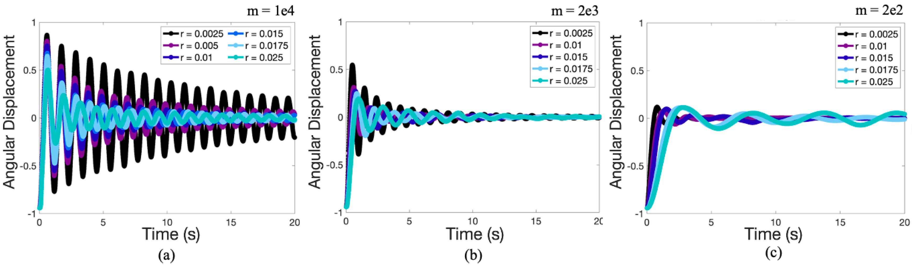
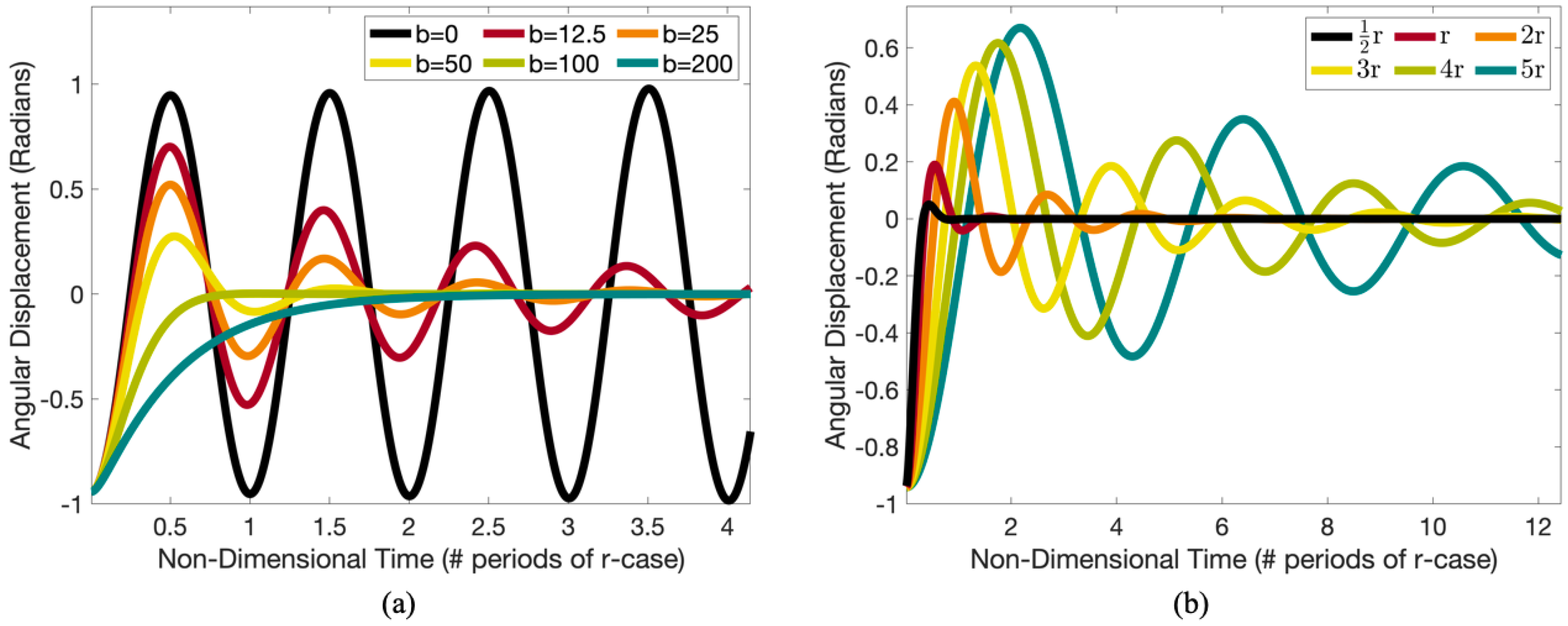
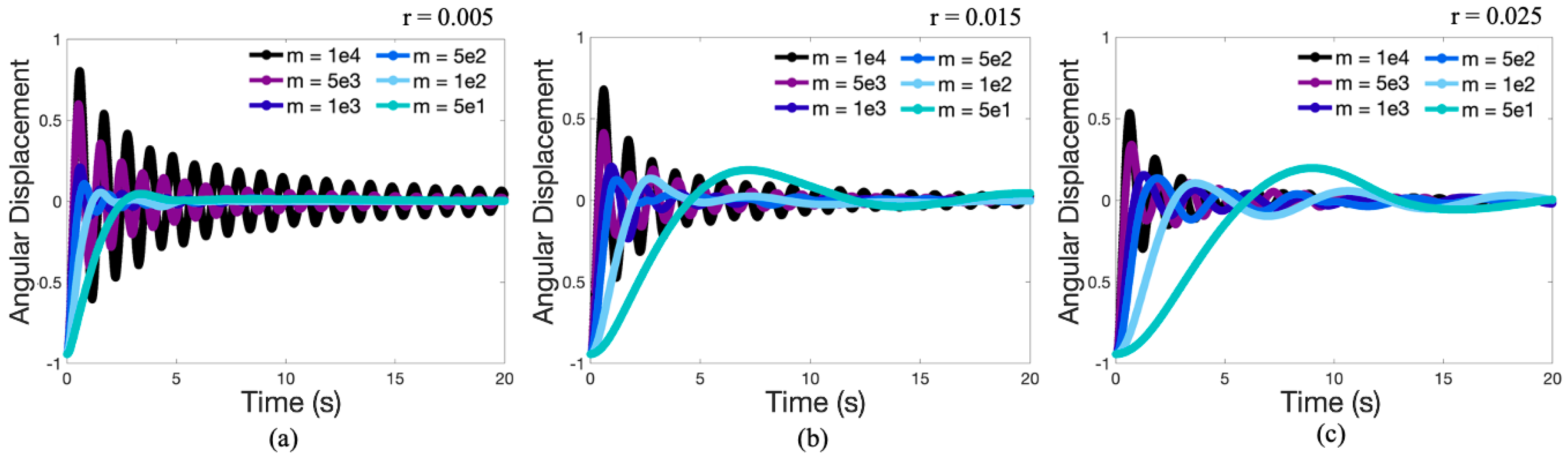
- Under-damped: The pendulum will swing back and forth, although its amplitude of oscillation will steadily decline, until it asymptotically approaches its equilibrium.
- Critically-damped: the pendulum returns to equilibrium as quickly as it can. If the damping parameter were made slightly more or slightly less, it would result in the pendulum returning slower to its equilibrium position.
- Over-damped: the pendulum moves towards its equilibrium position slower than the critically-damped case. There is no oscillation.
2. Methods
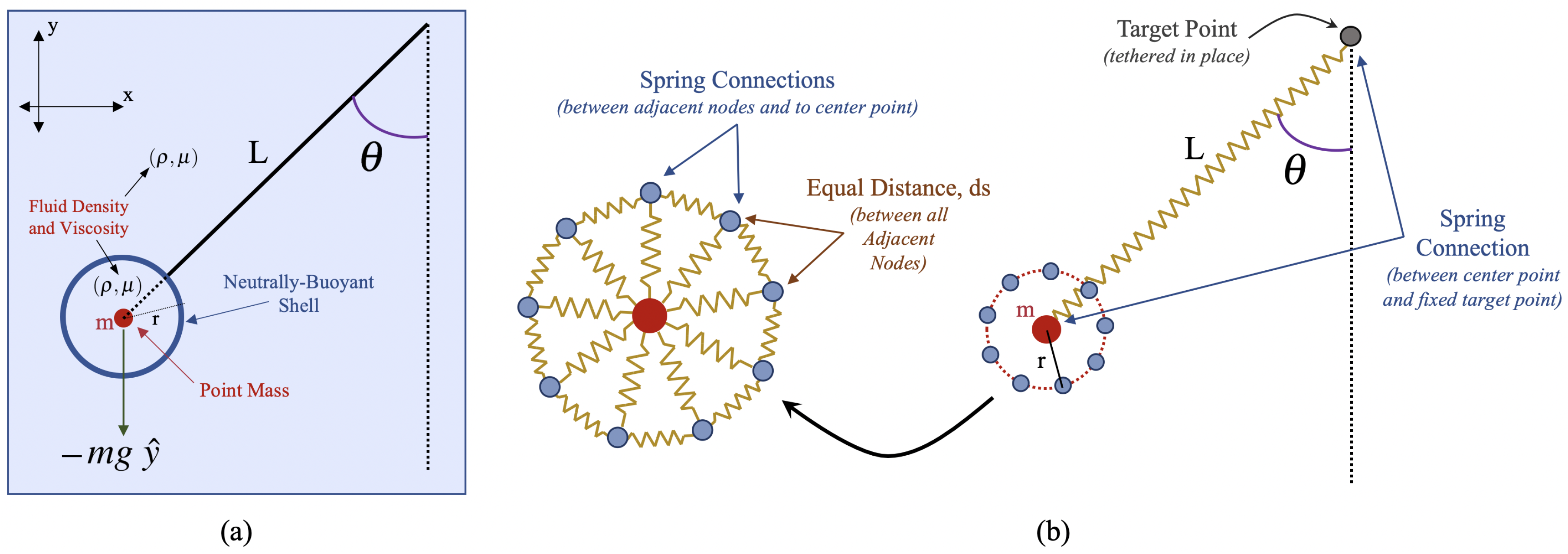
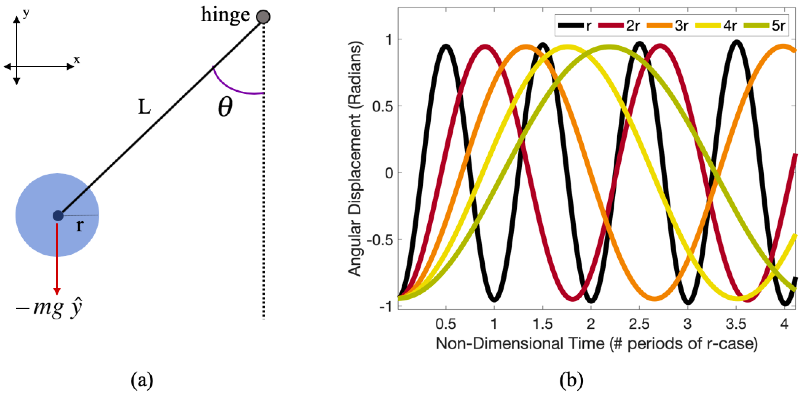
2.1. Model Geometry
2.2. Model Construction
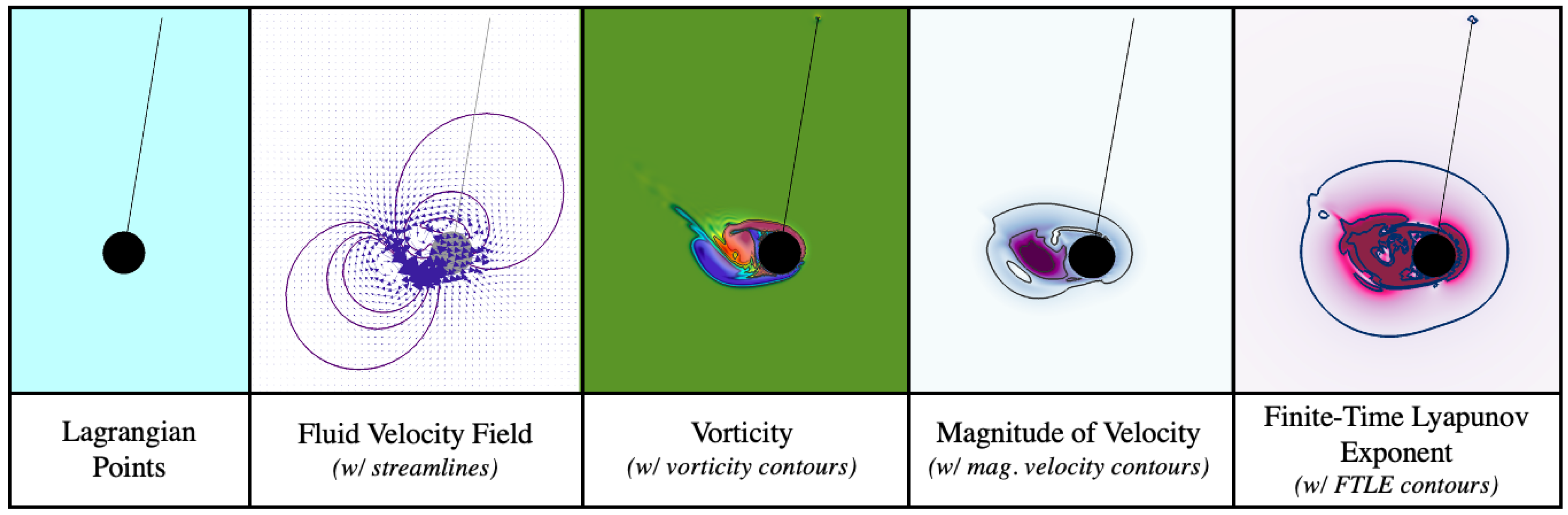
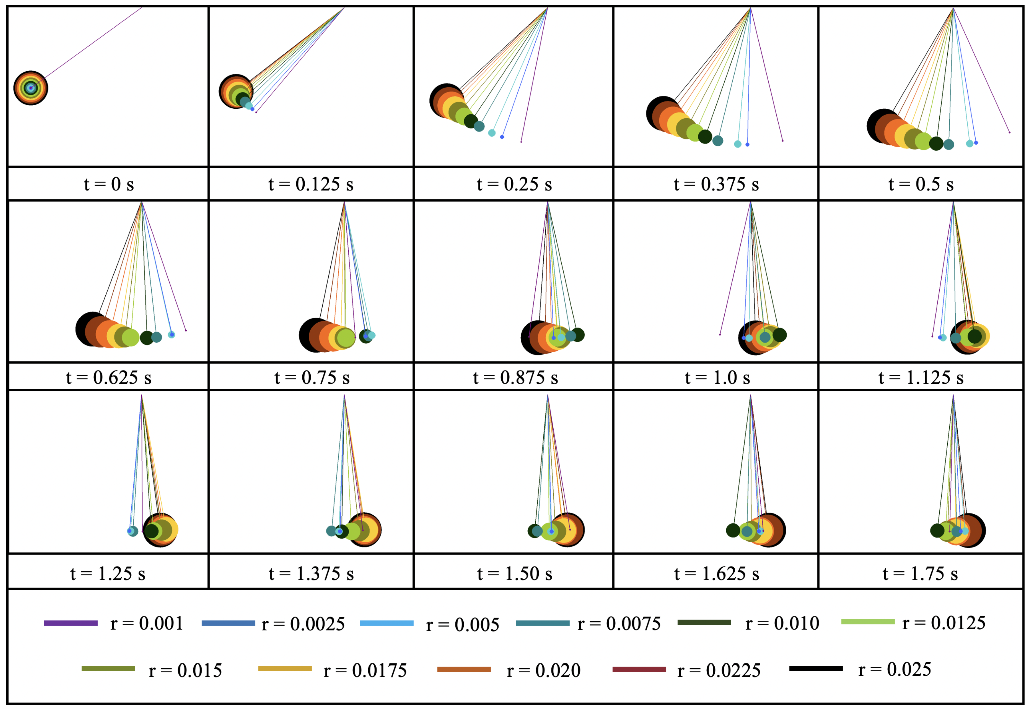
- Position of Lagrangian Points
- Forces on Each Lagrangian Point (Horizontal/Vertical and Normal/Tangential Forces)
- Fluid Velocity
- Fluid Vorticity
- Forces spread from the Lagrangian mesh onto the Eulerian grid
3. Results
- Angular Displacement of the pendulum bob
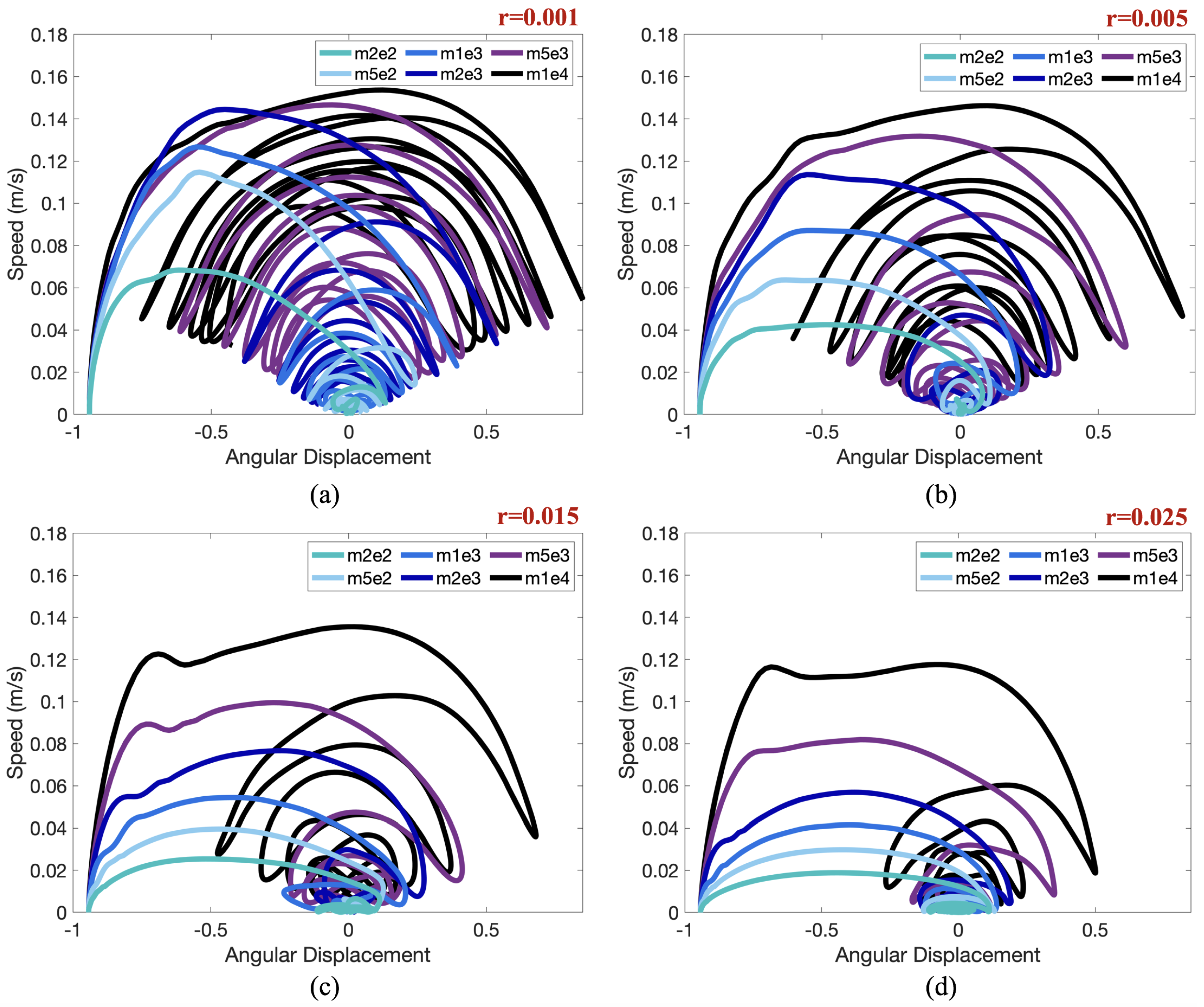
- Speed of the pendulum bob
- Forces acting on the pendulum bob
- Effect the pendulum bob has onto the fluid
- Comparison between reduced ODE model and FSI model
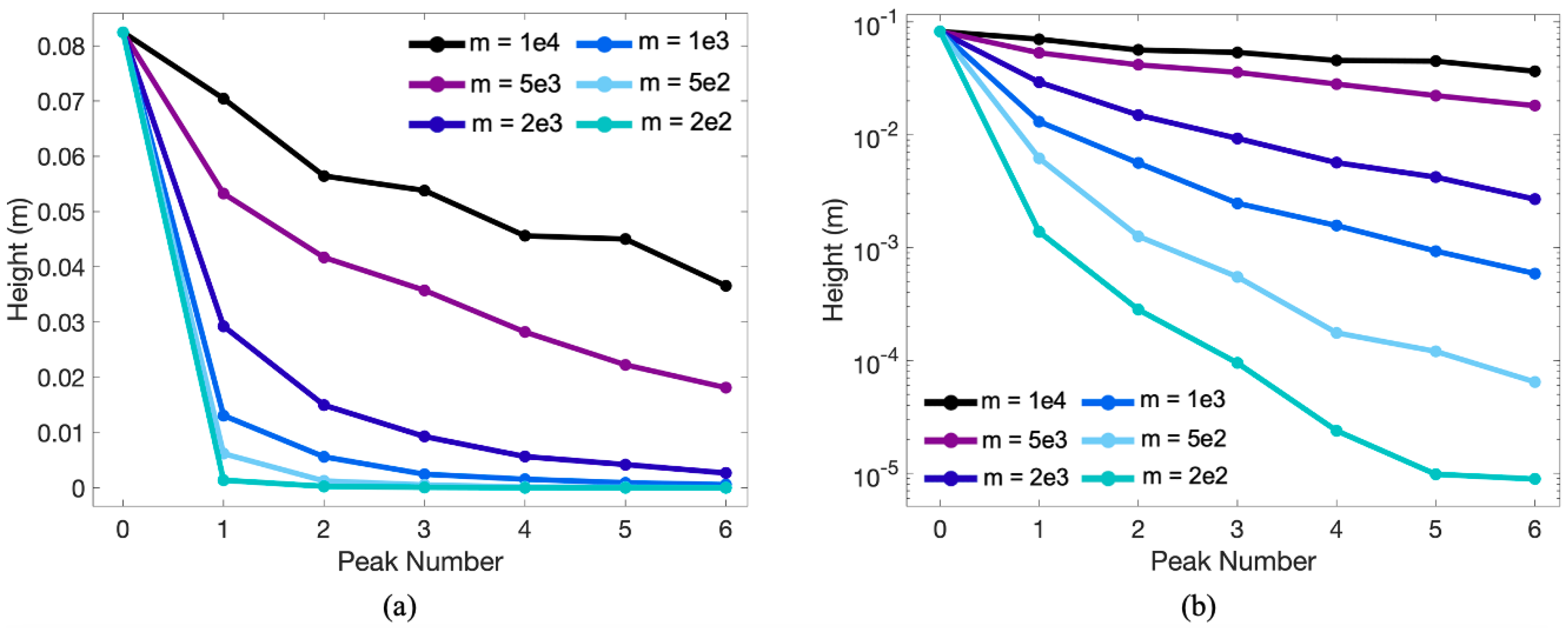
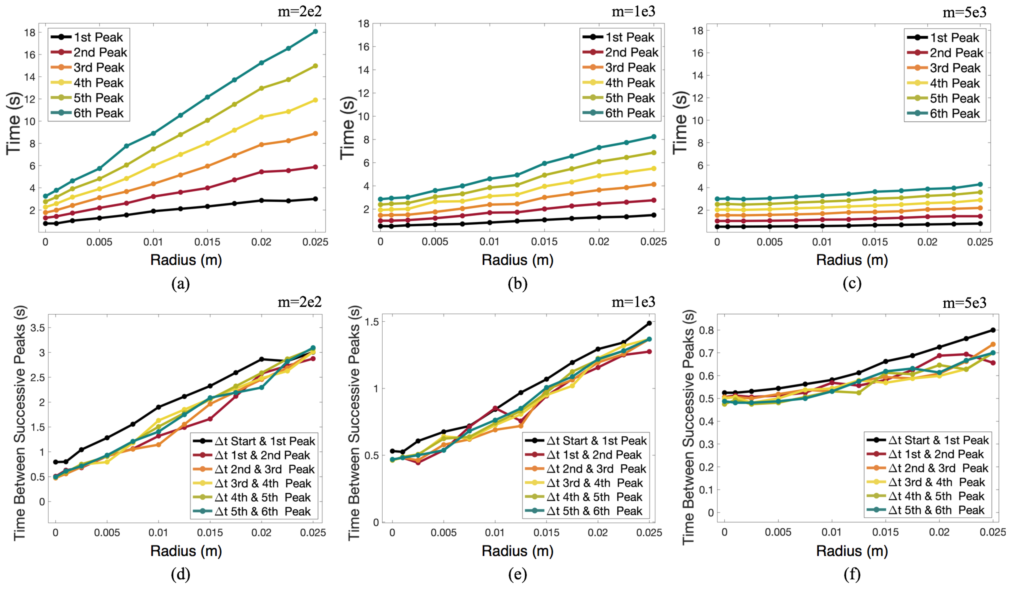
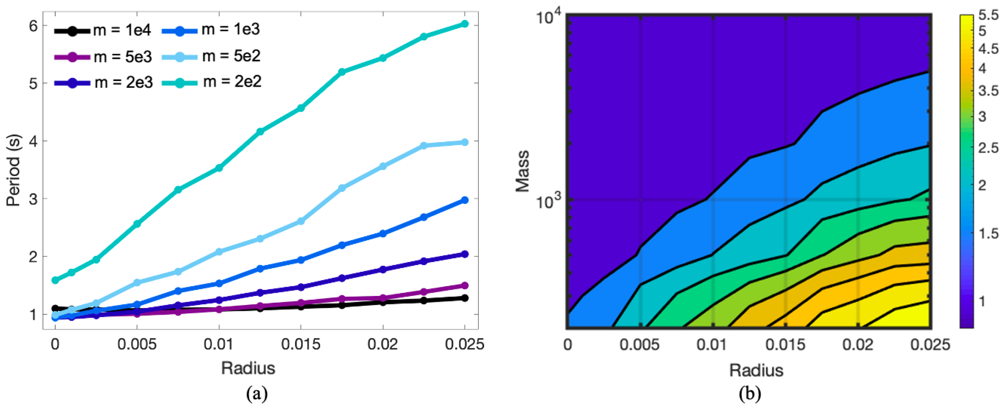
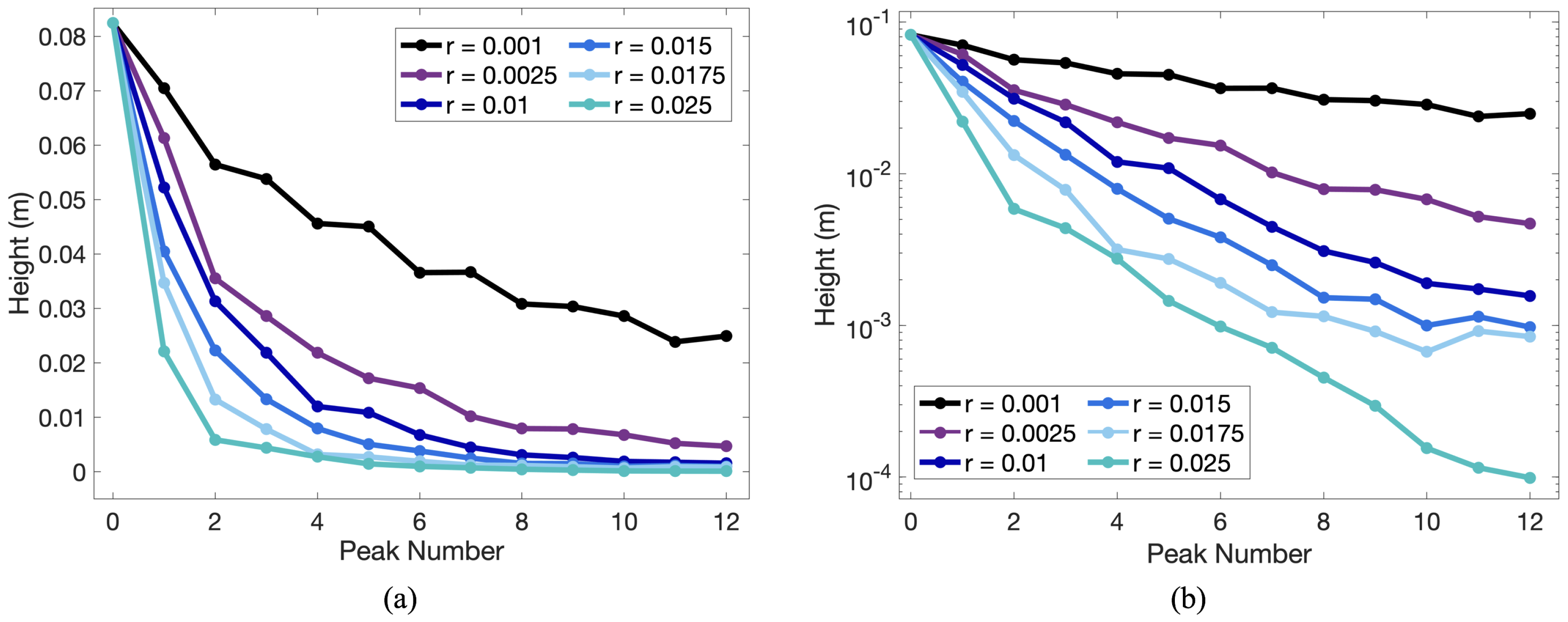
3.1. Angular Displacement of the Pendulum Bob
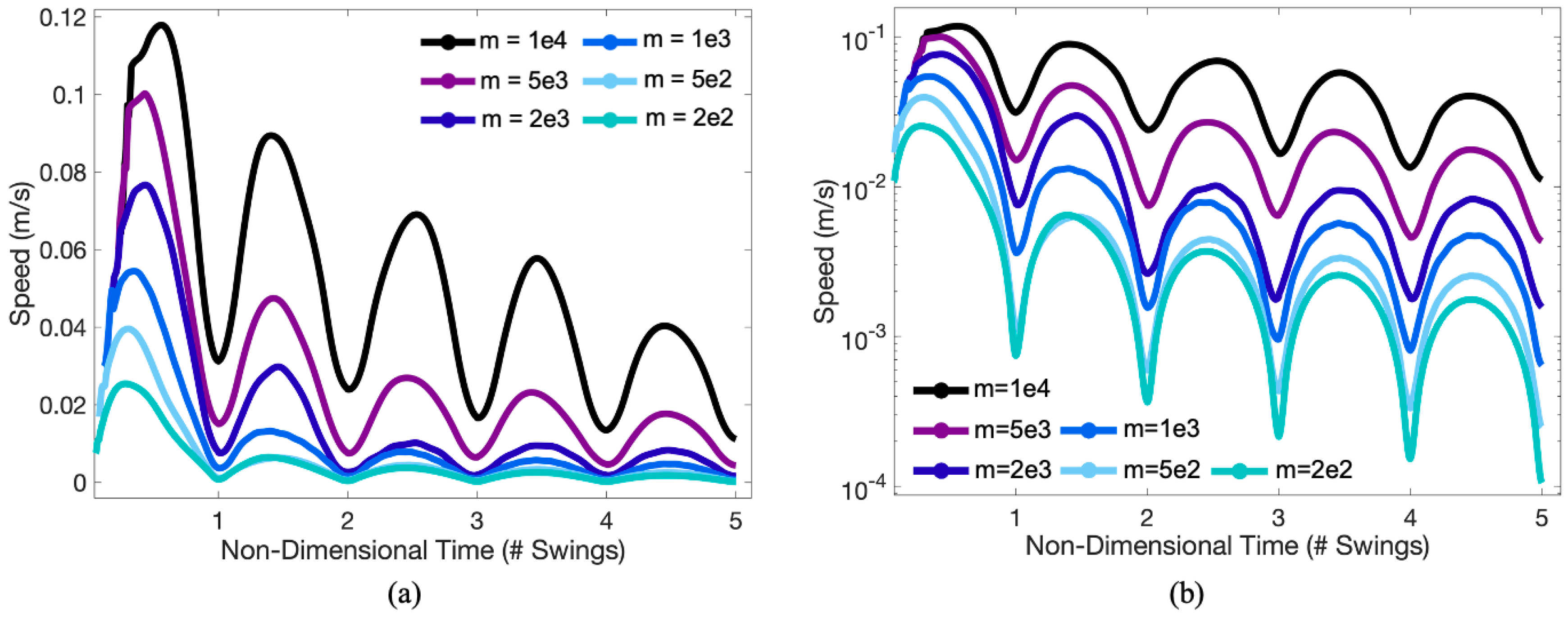
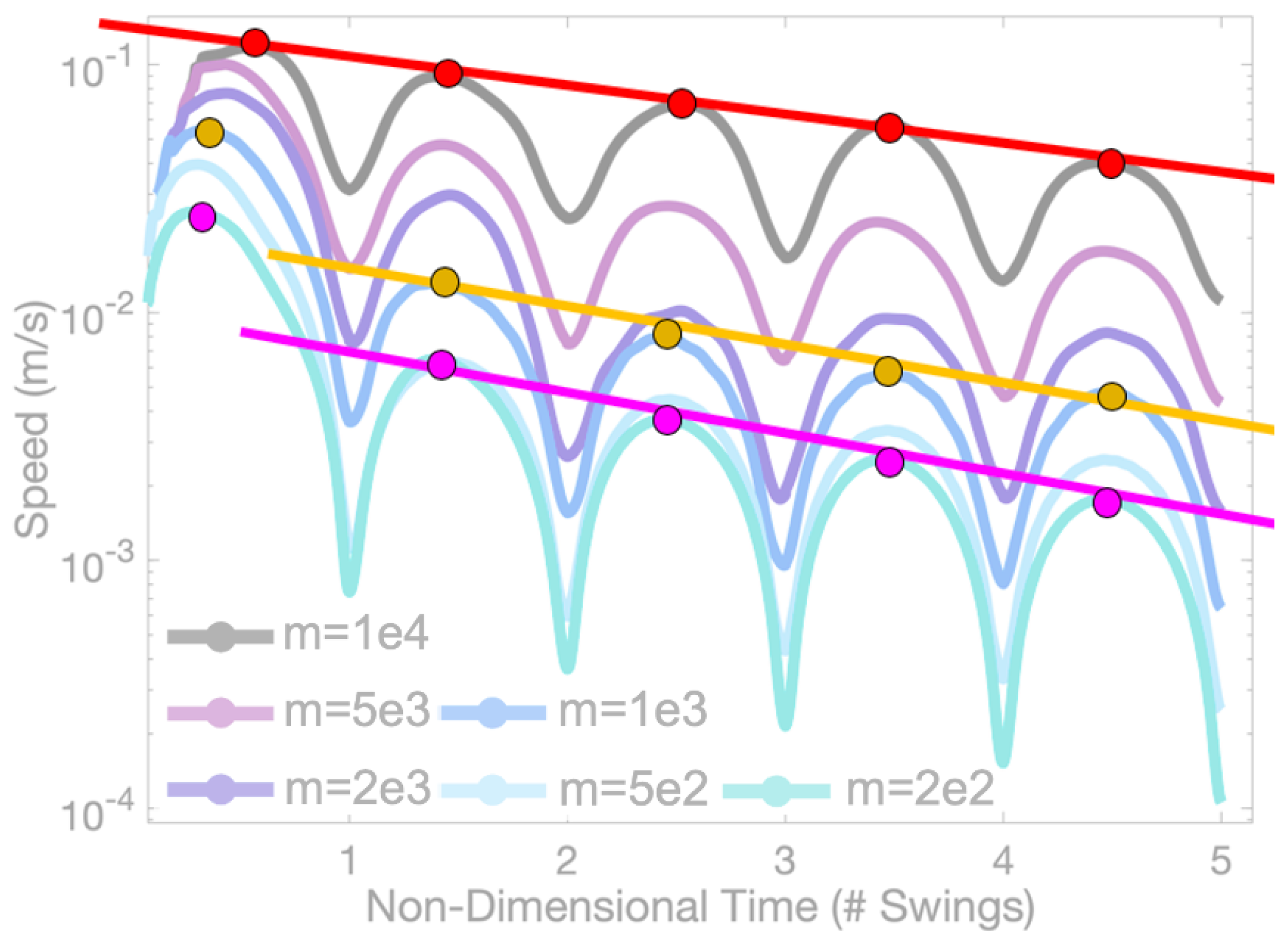
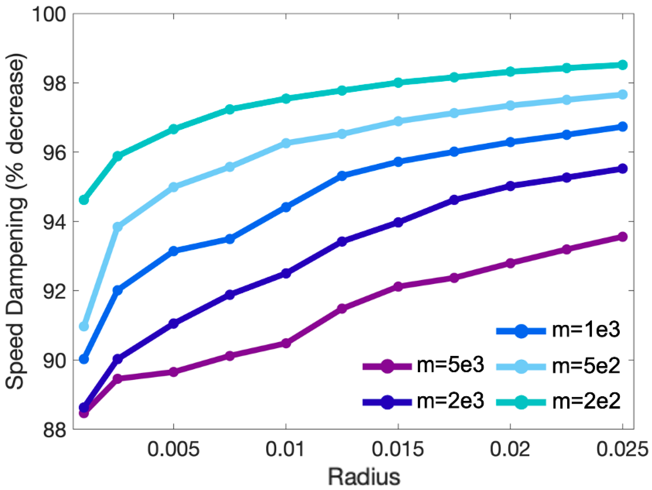
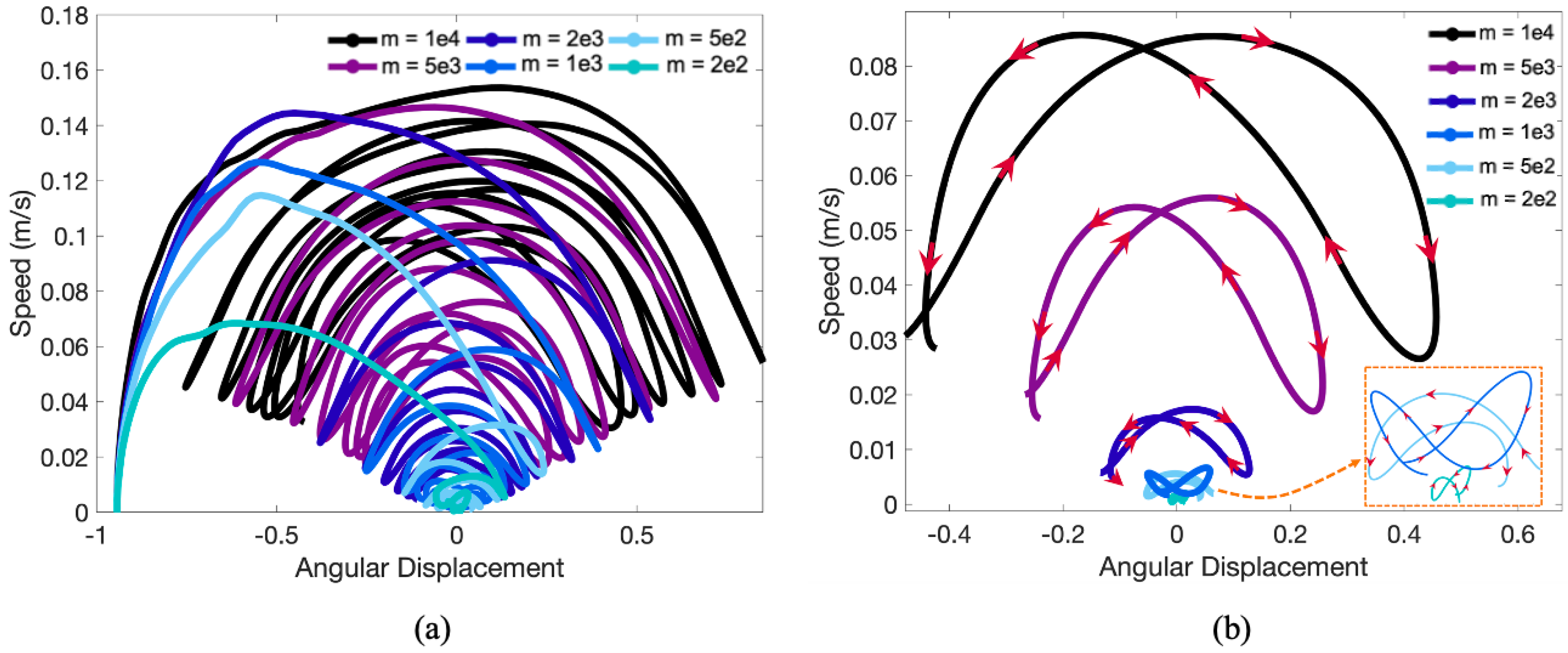
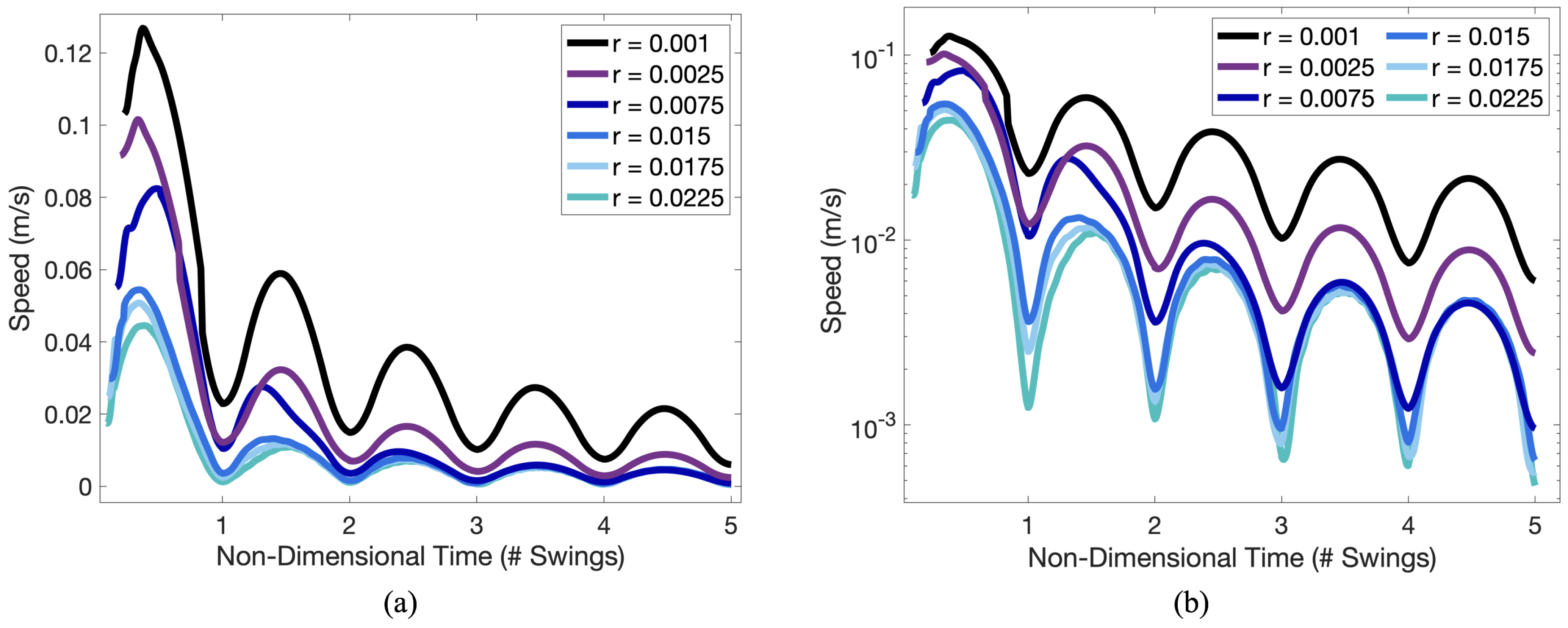
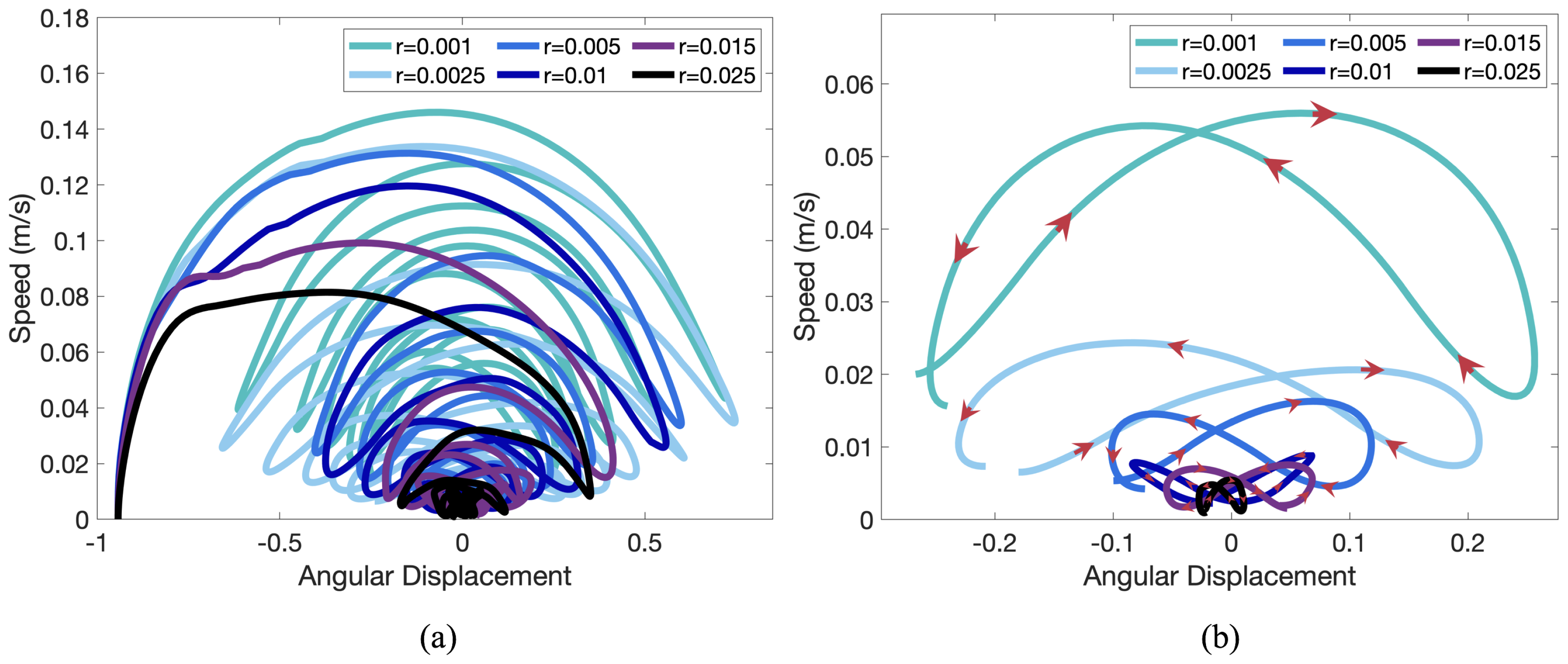
3.2. Speed of the Pendulum Bob
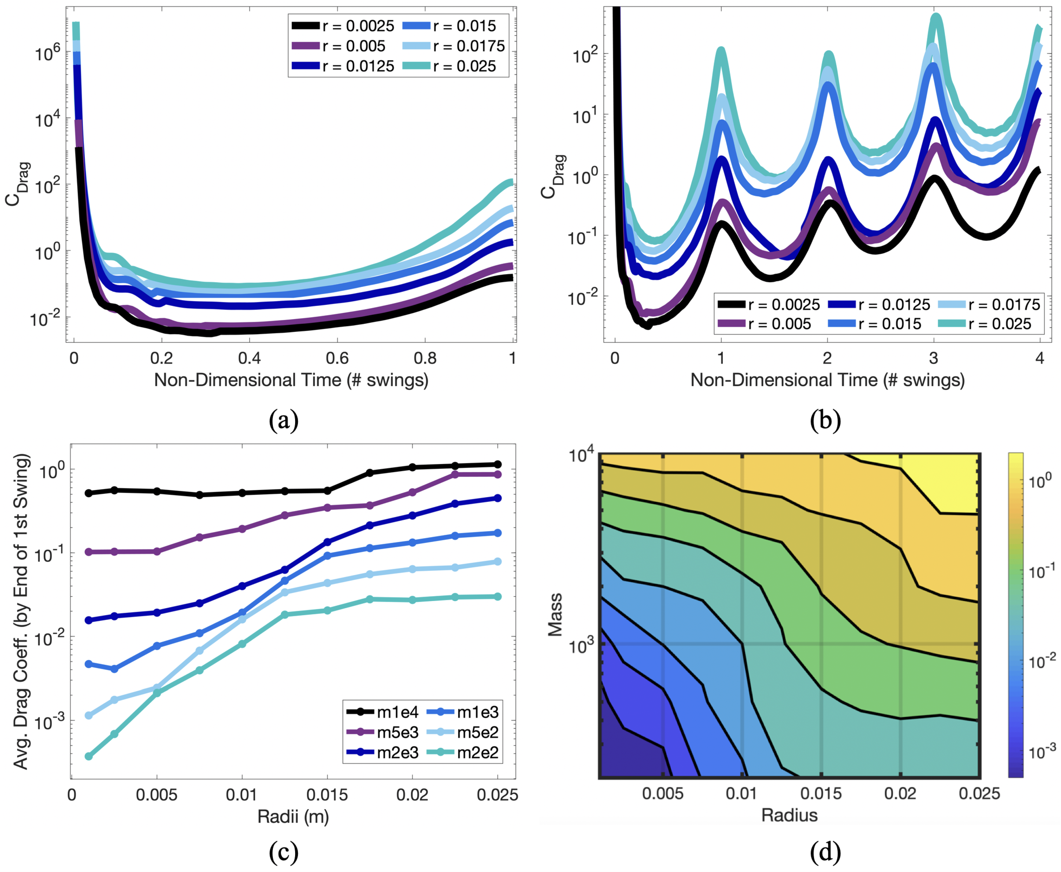
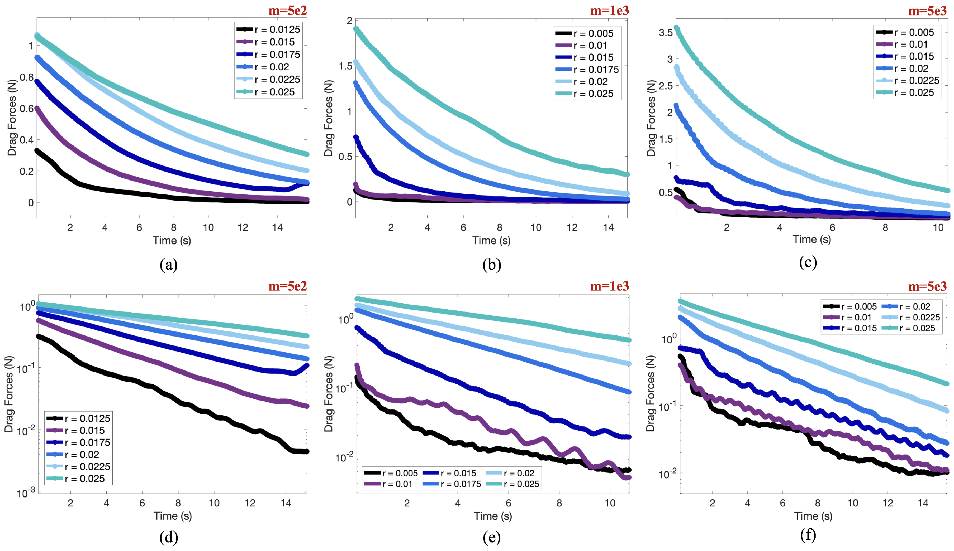
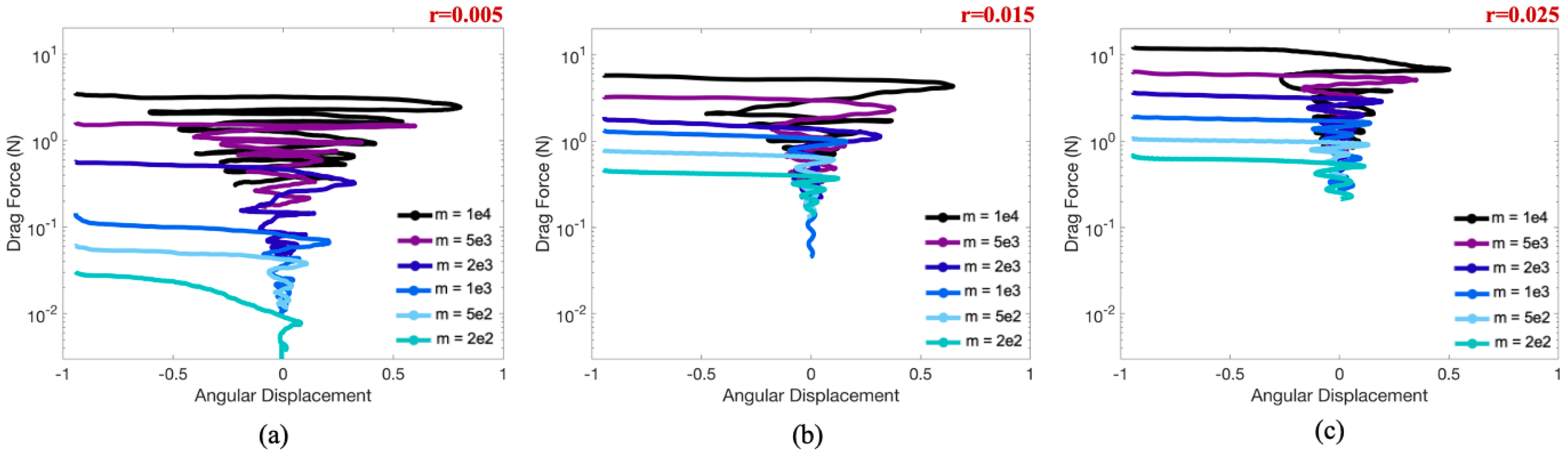
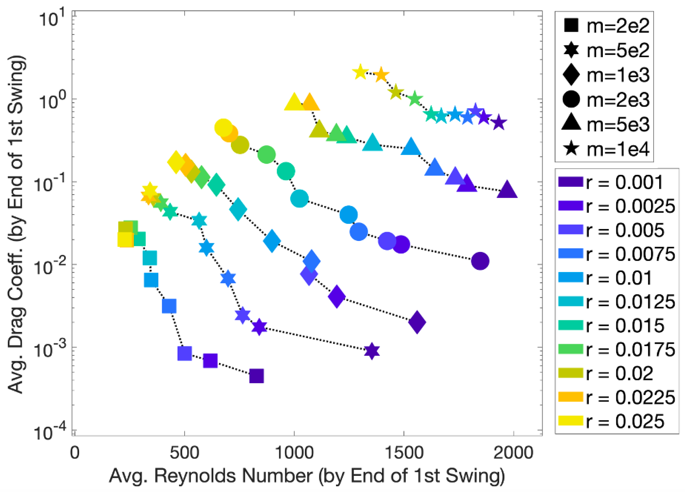
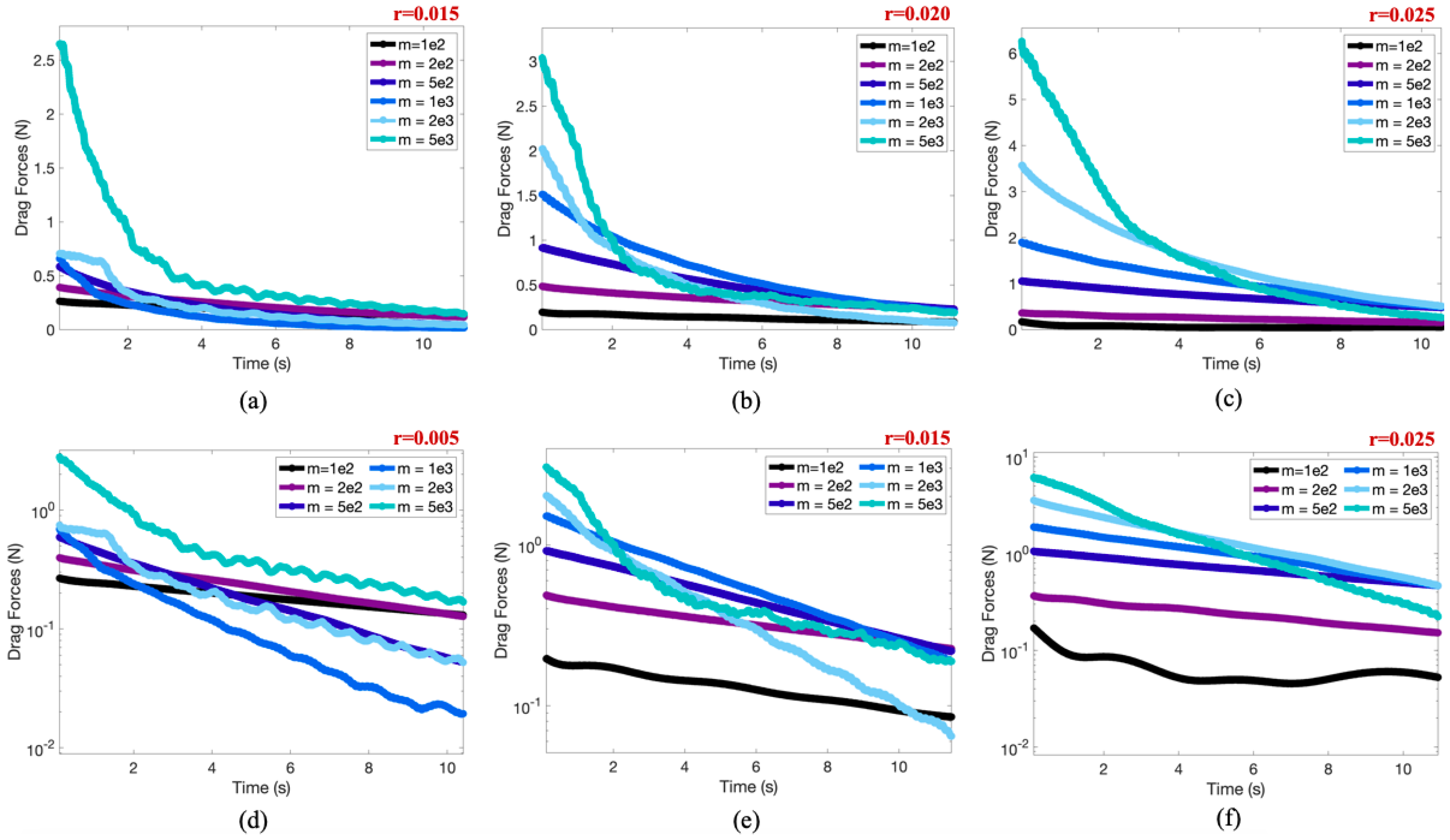
3.3. Forces on the Pendulum Bob
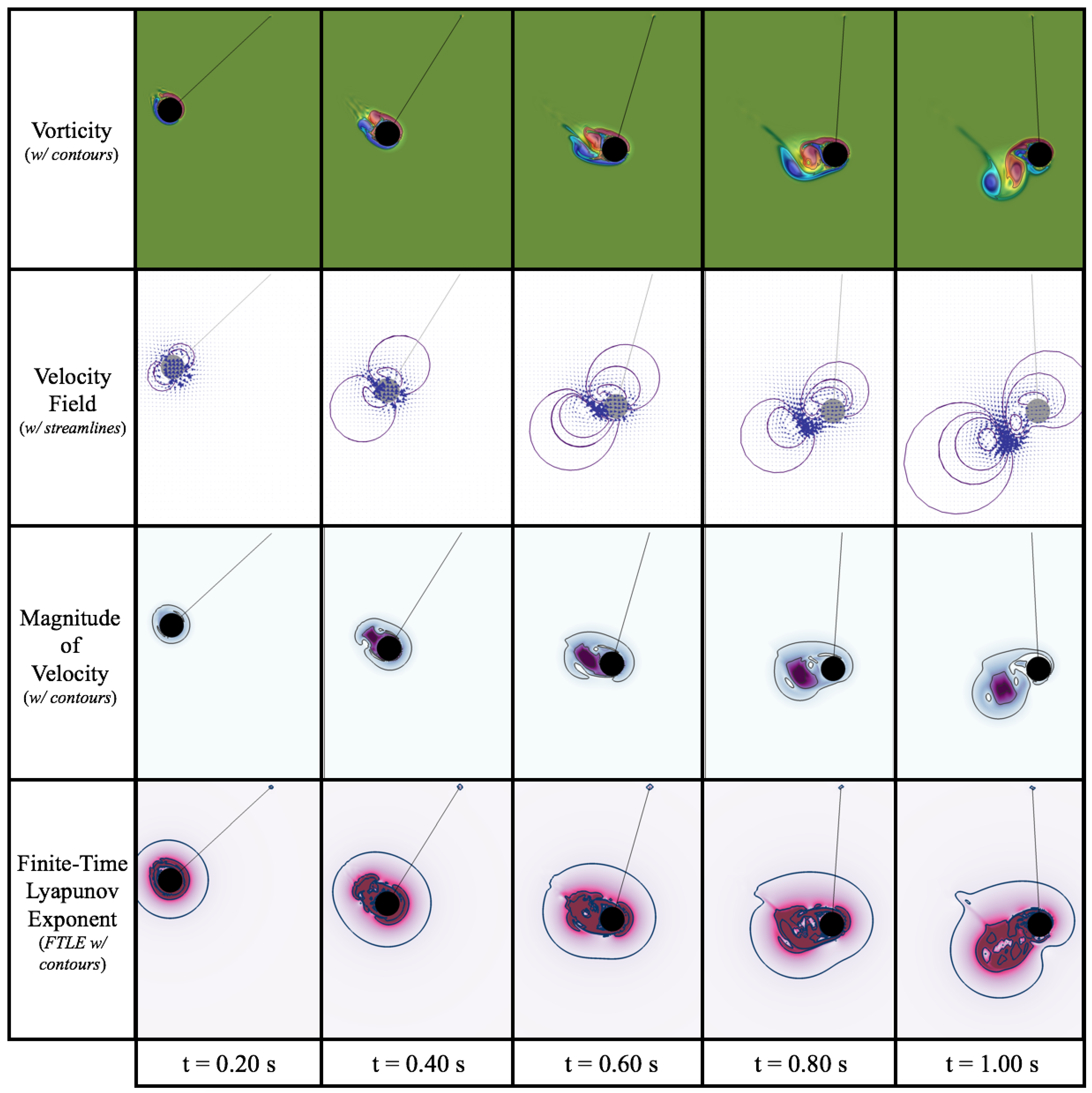
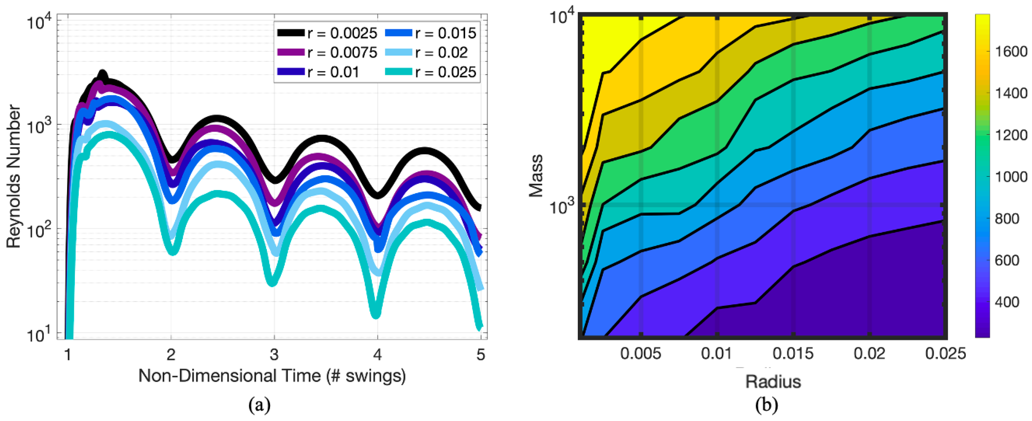
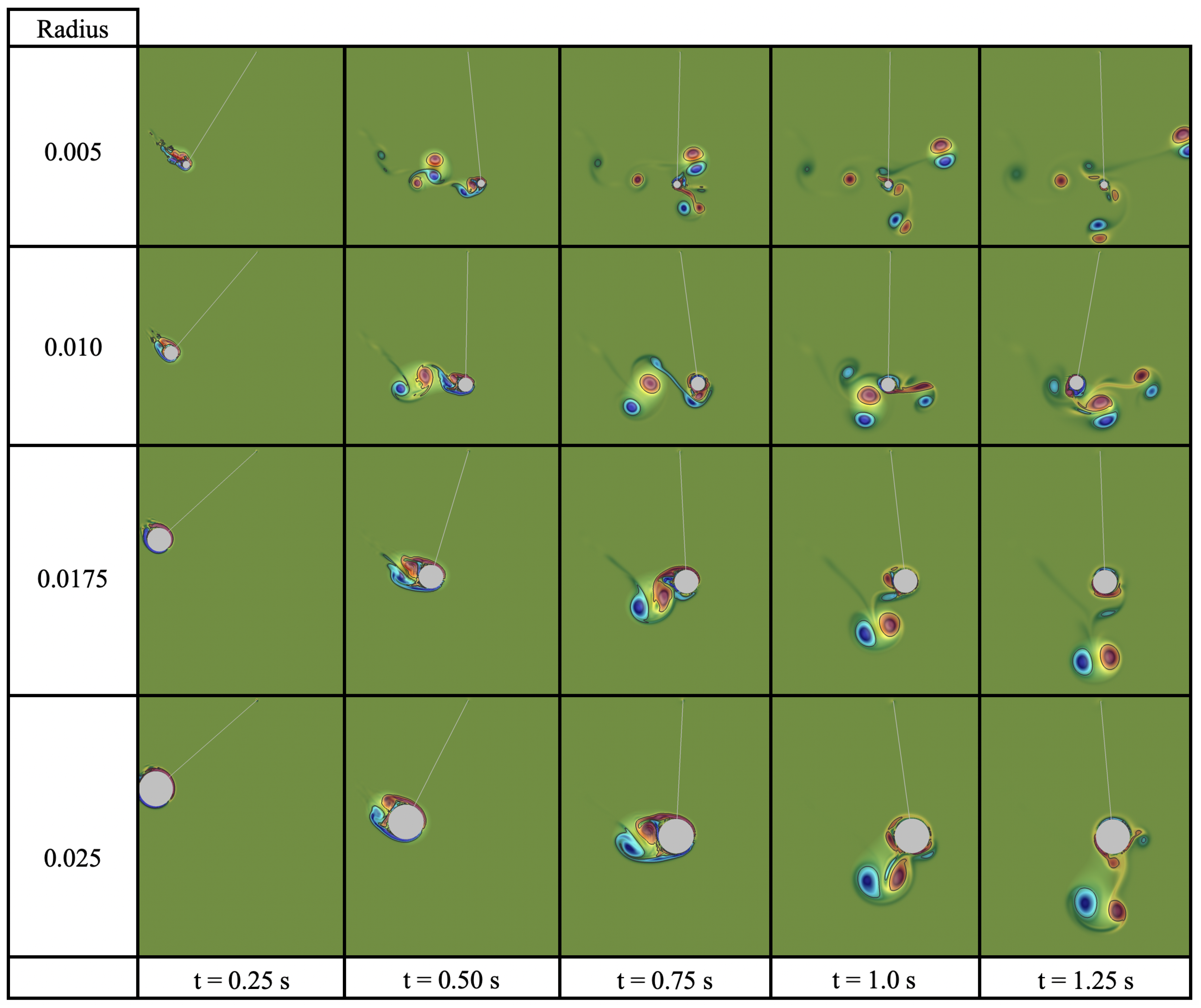
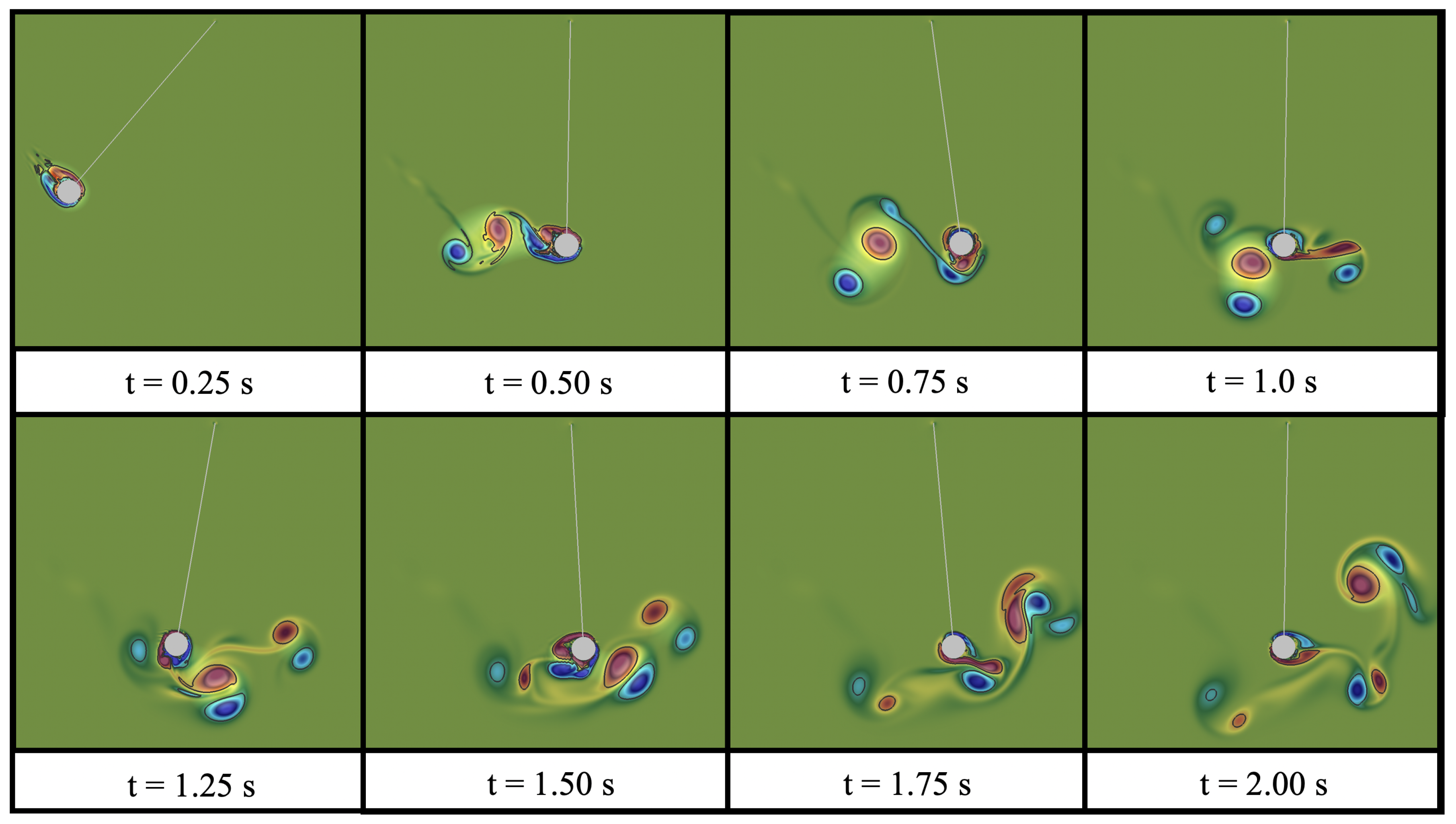
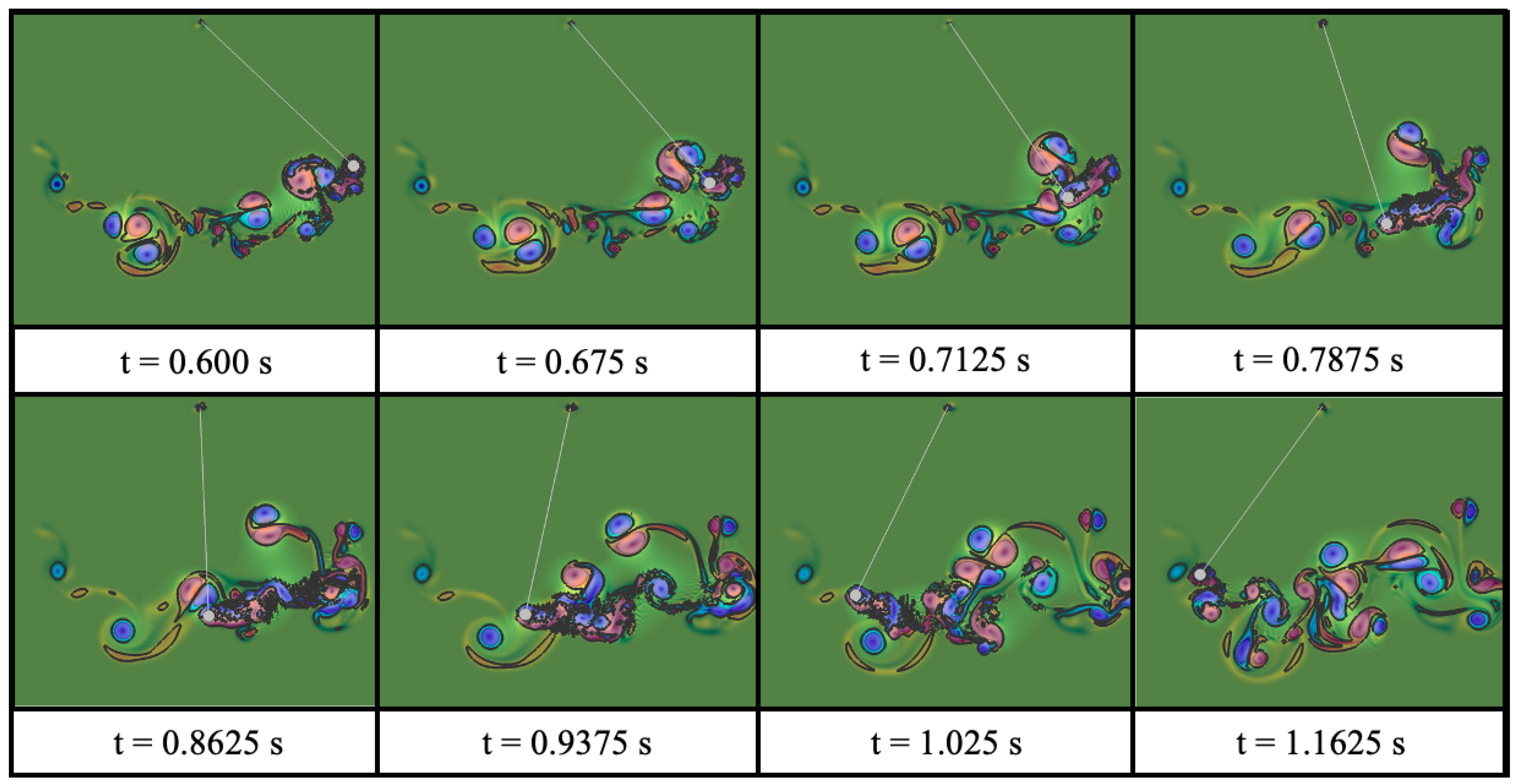
3.4. Effect the Pendulum Bob Has onto the Fluid
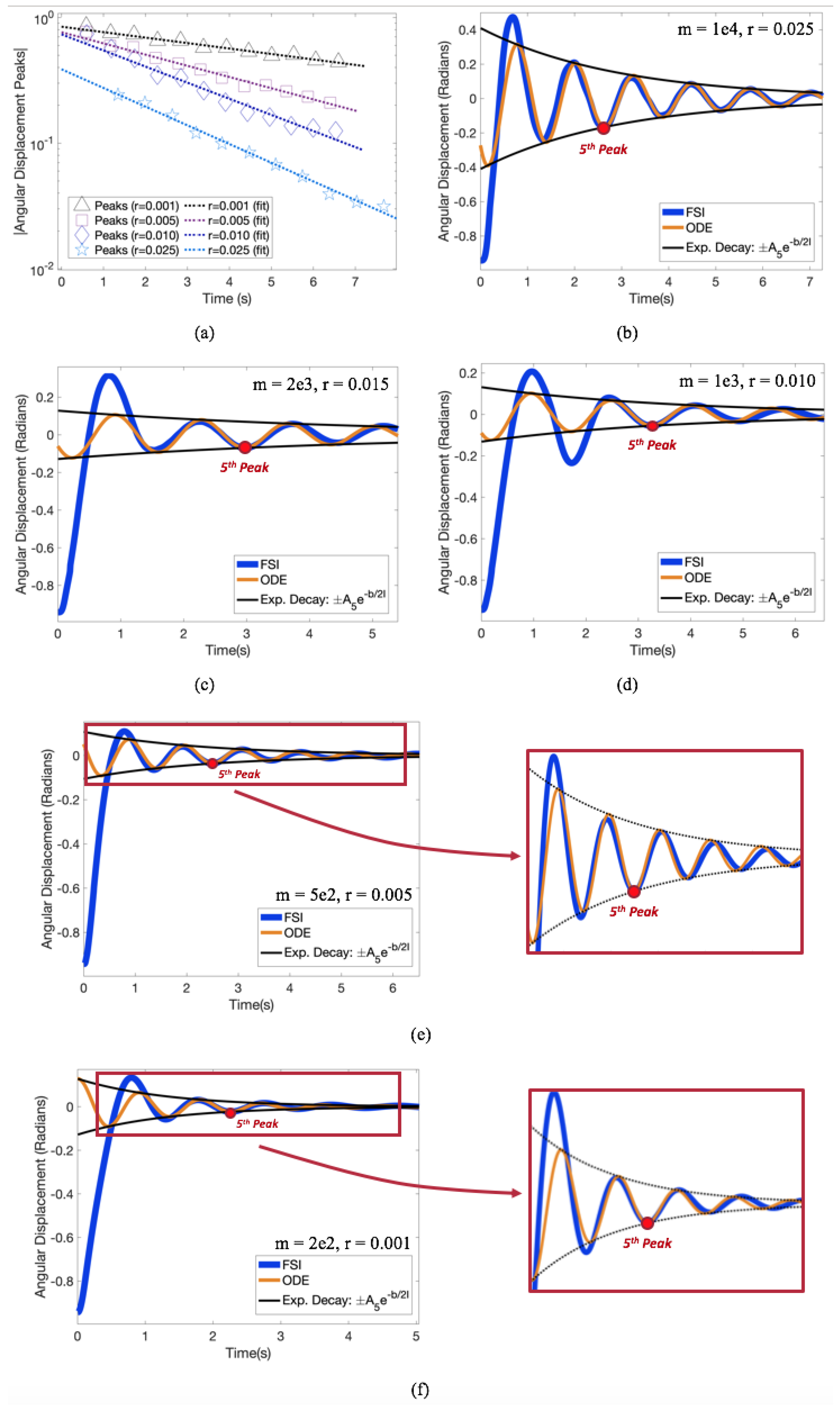
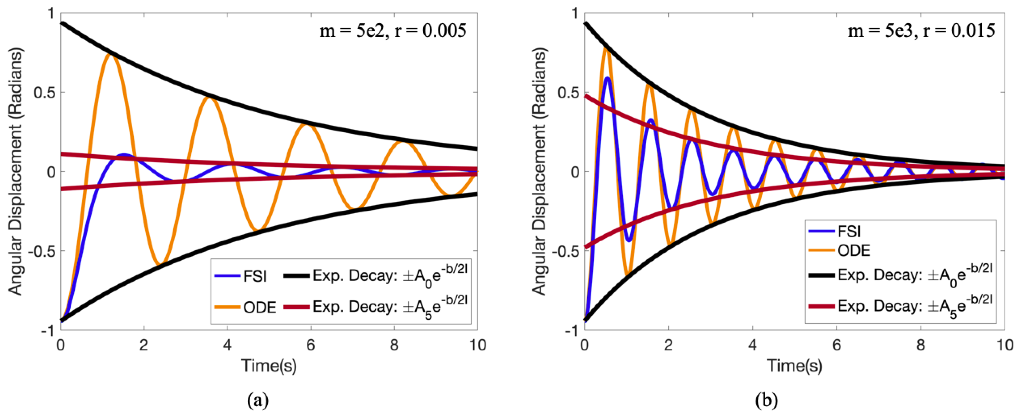
3.5. Numerical Comparison & Validation
4. Discussion and Conclusions
- A connection to where students may have seen fluid drag laws previously, i.e., the Stokes Drag Law and Pendulum Motion. Furthermore, it illustrates for students that famous laws of physics were discovered with systems that seem as “basic” as that of a pendulum.
- The differences that may arise between modeling a system using a reduced-order ODE model and attempting to computationally model all aspects of the system to a higher degree. We hope this shows students that reduced models are valuable in that they are usually easier to solve while (hopefully) capturing a bulk of a system’s dynamics. However, there are clear disadvantages as illustrated by the discrepancies that arise between the reduced order model and computational model—many dynamics are not captured in the reduced-model, e.g., the vortex wake or drafting, that maybe particularly interesting or important to understanding the system as a whole.
- Similarly, the full dynamical richness of a system may only be explored by investigating its explicit fluid mechanics, even in a system as seemingly “simple” as a single pendulum immersed in a fluid. Moreover, to even study systems involving fluids and objects immersed therein, it requires either sophisticated experimental techniques or computational expertise. This work shows that a computer can be an immensely powerful tool for performing science. More than that, programming knowledge is highly sought after in this day and age [83,84].
- The observation that even systems that are routinely studied in some introductory courses, like a pendulum, may still have open, exciting research questions that scientists and engineers actively pursue.
Supplementary Materials
Author Contributions
Funding
Acknowledgments
Conflicts of Interest
Abbreviations
| CFD | Computational Fluid Dynamics |
| FSI | Fluid-Structure Interaction |
| Re | Reynolds Number |
| IB | Immersed Boundary Method |
| ODE | Ordinary Differential Equation |
Appendix A. Instructor Resources
- Pendulum_Classroom_Supplement.pptx/.pdf: presentations which may be used in class; slides that tell the story of the paper. Note that the file has embedded movies in format.
- Movies: directory containing movies ( format) pertaining to each simulation shown in the manuscript.
- Note that an open-source fluid-structure interaction model of a point-mass pendulum can be found at: https://github.com/nickabattista/IB2d in the sub-directory:IB2d → matIB2d → Examples → Examples_Education→ Pendulum.
- Visualization software used: VisIt (https://visit.llnl.gov/) (v. 2.12.3)
Appendix B. Immersed Boundary Method
IB Algorithm
Appendix C. Additional Pendulum Data


References
- Milne, J. Pendulum Seismometers. Nature 1888, 37, 570–571. [Google Scholar] [CrossRef] [Green Version]
- Morton, W.S.; Lewis, C.M. China: Its History and Culture; McGraw-Hill, Inc.: New York, NY, USA, 2005. [Google Scholar]
- Matthews, M.R. Time for Science Education: How Teaching the History and Philosophy of Pendulum Motion Can Contribute to Science Literacy; Springer: New York, NY, USA, 2000. [Google Scholar]
- Blackwell, N. Experimental stone-cutting with the Mycenaean pendulum saw. Antiquity 2018, 92, 217–232. [Google Scholar] [CrossRef]
- Bennett, M.; Schatz, M.F.; Rockwood, H.; Wiesenfeld, K. Huygens’ Clocks. Proc. R. Soc. Lond. A 2002, 458, 563–579. [Google Scholar] [CrossRef]
- Boettcher, W.; Merkle, F.; Weitkemper, H.H. History of extracorporeal circulation: The conceptional and developmental period. J. Extra Corpor. Technol. 2003, 3, 172–183. [Google Scholar]
- Scott, G.R. The History of Torture throughout the Ages; Kessinger Publishing, LLC: Whitefish, MT, USA, 2009. [Google Scholar]
- Poe, E.A. The Pit and the Pendulum. In The Gift: A Christmas and New Year’s Present for 1843; Leslie, E., Ed.; Carey & Hart: Philadelphia, PA, USA, 1843; Chapter 12; pp. 133–152. [Google Scholar]
- Halliday, D.; Resnick, R.; Walker, J. Fundamentals of Physics, 7th ed.; John Wiley & Sons: New York, NY, USA, 2004. [Google Scholar]
- Stokes, G.G. On the Effect of the Internal Friction of Fluids on the Motion of Pendulums. Trans. Camb. Philos. Soc. 1851, 9, 8–106. [Google Scholar]
- Batchelor, G.K. Introduction to Fluid Mechanics; Cambridge University Press: Cambridge, UK, 2000. [Google Scholar]
- Happel, J.; Brenner, H. Low Reynolds Number Hydrodynamics; Springer: New York, NY, USA, 1981. [Google Scholar]
- Buckingham, E. On physically similar systems; illustrations of the use of dimensional equations. Phys. Rev. 2014, 4, 245–376. [Google Scholar] [CrossRef]
- Landau, L.D.; Lifshitz, E.M. Fluid Mechanics, 1st ed.; Pergamon: London, UK, 1959. [Google Scholar]
- Mahajan, S. Chapter 4: Fluid Drag. Notes from MIT IAP Course in 2006: Lies and Damn Lies: The Art of Approximation in Science. 2006. Available online: http://www.inference.org.uk/sanjoy/mit/book:04.pdf (accessed on 3 January 2020).
- Nelson, R.A.; Olsson, M.G. The Pendulum-Rich physics from a simple system. Am. J. Phys. 1986, 2, 54. [Google Scholar] [CrossRef]
- Peters, R.D. Nonlinear Damping of the ‘Linear’ Pendulum. 2003. Available online: https://arxiv.org/abs/physics/0306081 (accessed on 15 December 2019).
- Peters, R.D. The Pendulum in the 21st Century-Relic or Trendsetter. Sci. Educ. 2004, 13, 279–295. [Google Scholar] [CrossRef]
- Quiroga, G.D.; Ospina-Henao, P.A. Dynamics of damped oscillations: Physical pendulum. Eur. J. Phys. 2017, 38, 065005. [Google Scholar] [CrossRef]
- Hsu, H.; Capart, H. Enhanced upswing in immersed collisions of tethered spheres. Phys. Fluids 2007, 19, 101701. [Google Scholar] [CrossRef] [Green Version]
- Neill, D.; Livelybrooks, D.; Donnelly, R.J. A pendulum experiment on added mass and the principle of equivalence. Am. J. Phys. 2007, 75, 226. [Google Scholar] [CrossRef]
- Sullivan, I.; Niemela, J.; Hershberger, R.; Bolster, D.; Donnelly, R. Dynamics of thin vortex rings. J. Fluid Mech. 2008, 609, 319–347. [Google Scholar] [CrossRef] [Green Version]
- Bolster, D.; Hershberger, R.E.; Donnelly, R.J. Oscillating pendulum decay by emission of vortex rings. Phys. Rev. E 2010, 13, 046317. [Google Scholar] [CrossRef] [PubMed] [Green Version]
- Bandi, M.M.; Concha, A.; Wood, R.; Mahadevan, L. A pendulum in a flowing soap film. Phys. Fluids 2013, 25, 041702. [Google Scholar] [CrossRef]
- Mathai, V.; Loeffen, L.; Chan, T.; Wildeman, S. Dynamics of heavy and buoyant underwater pendulums. J. Fluid Mech. 2019, 862, 348–363. [Google Scholar] [CrossRef] [Green Version]
- Farnell, D.J.; David, R.; Barton, D.C. Numerical simulations of a filament in a flowing soap film. Int. J. Numer. Methods Fluids 2004, 44, 313–330. [Google Scholar] [CrossRef]
- Orchini, A.; Kellay, H.; Mazzino, A. Galloping instability and control of a rigid pendulum in a flowing soap film. J. Fluids Struct. 2015, 56, 124–133. [Google Scholar] [CrossRef] [Green Version]
- Peskin, C. Flow patterns around heart valves: A numerical method. J. Comput. Phys. 1972, 10, 252–271. [Google Scholar] [CrossRef]
- Peskin, C. Numerical analysis of blood flow in the heart. J. Comput. Phys. 1977, 25, 220–252. [Google Scholar] [CrossRef]
- Peskin, C.S. The immersed boundary method. Acta Numer. 2002, 11, 479–517. [Google Scholar] [CrossRef] [Green Version]
- Fauci, L.; Fogelson, A. Truncated Newton methods and the modeling of complex immersed elastic structures. Commun. Pure Appl. Math 1993, 46, 787–818. [Google Scholar] [CrossRef]
- Lai, M.C.; Peskin, C.S. An Immersed Boundary Method with Formal Second-Order Accuracy and Reduced Numerical Viscosity. J. Comput. Phys. 2000, 160, 705–719. [Google Scholar] [CrossRef] [Green Version]
- Cortez, R.; Minion, M. The Blob Projection Method for Immersed Boundary Problems. J. Comput. Phys. 2000, 161, 428–453. [Google Scholar] [CrossRef] [Green Version]
- Griffith, B.E.; Peskin, C.S. On the order of accuracy of the immersed boundary method: Higher order convergence rates for sufficiently smooth problems. J. Comput. Phys. 2005, 208, 75–105. [Google Scholar] [CrossRef]
- Mittal, R.; Iaccarino, C. Immersed boundary methods. Annu. Rev. Fluid Mech. 2005, 37, 239–261. [Google Scholar] [CrossRef] [Green Version]
- Griffith, B.E.; Hornung, R.; McQueen, D.; Peskin, C.S. An adaptive, formally second order accurate version of the immersed boundary method. J. Comput. Phys. 2007, 223, 10–49. [Google Scholar] [CrossRef]
- Griffith, B.E. An Adaptive and Distributed-Memory Parallel Implementation of the Immersed Boundary (IB) Method. 2014. Available online: https://github.com/IBAMR/IBAMR (accessed on 21 October 2014).
- Griffith, B.E.; Luo, X. Hybrid finite difference/finite element version of the immersed boundary method. Int. J. Numer. Methods Biomed. Eng. 2017, 33, e2888. [Google Scholar] [CrossRef] [Green Version]
- Battista, N.A.; Strickland, W.C.; Miller, L.A. IB2d: A Python and MATLAB implementation of the immersed boundary method. Bioinspir. Biomim. 2017, 12, 036003. [Google Scholar] [CrossRef] [Green Version]
- Battista, N.A.; Strickland, W.C.; Barrett, A.; Miller, L.A. IB2d Reloaded: A more powerful Python and MATLAB implementation of the immersed boundary method. Math. Methods Appl. Sci. 2018, 41, 8455–8480. [Google Scholar] [CrossRef] [Green Version]
- Miller, L.A. Fluid Dynamics of Ventricular Filling in the Embryonic Heart. Cell Biochem. Biophys. 2011, 61, 33–45. [Google Scholar] [CrossRef]
- Griffith, B.E. Immersed boundary model of aortic heart valve dynamics with physiological driving and loading conditions. Int. J. Numer. Methods Biomed. Eng. 2012, 28, 317–345. [Google Scholar] [CrossRef] [PubMed] [Green Version]
- Battista, N.A.; Lane, A.N.; Liu, J.; Miller, L.A. Fluid Dynamics of Heart Development: Effects of Trabeculae and Hematocrit. Math. Med. Biol. 2017, 35, 493–516. [Google Scholar] [CrossRef] [PubMed] [Green Version]
- Battista, N.A.; Douglas, D.R.; Lane, A.N.; Samsa, L.A.; Liu, J.; Miller, L.A. Vortex Dynamics in Trabeculated Embryonic Ventricles. J. Cardiovasc. Dev. Dis. 2019, 6, 6. [Google Scholar] [CrossRef] [PubMed] [Green Version]
- Bhalla, A.; Griffith, B.E.; Patankar, N. A forced damped oscillation framework for undulatory swimming provides new insights into how propulsion arises in active and passive swimming. PLoS Comput. Biol. 2013, 9, e1003097. [Google Scholar] [CrossRef] [Green Version]
- Bhalla, A.; Griffith, B.E.; Patankar, N. A unified mathematical frame- work and an adaptive numerical method for fluid-structure interaction with rigid, deforming, and elastic bodies. J. Comput. Phys. 2013, 250, 446–476. [Google Scholar] [CrossRef]
- Hamlet, C.; Fauci, L.J.; Tytell, E.D. The effect of intrinsic muscular nonlinearities on the energetics of locomotion in a computational model of an anguilliform swimmer. J. Theor. Biol. 2015, 385, 119–129. [Google Scholar] [CrossRef] [Green Version]
- Hoover, A.P.; Griffith, B.E.; Miller, L.A. Quantifying performance in the medusan mechanospace with an actively swimming three-dimensional jellyfish model. J. Fluid Mech. 2017, 813, 1112–1155. [Google Scholar] [CrossRef]
- Miles, J.G.; Battista, N.A. Naut your everyday jellyfish model: Exploring how tentacles and oral arms impact locomotion. Fluids 2019, 4, 169. [Google Scholar] [CrossRef] [Green Version]
- Miller, L.A.; Peskin, C.S. When vortices stick: An aerodynamic transition in tiny insect flight. J. Exp. Biol. 2004, 207, 3073–3088. [Google Scholar] [CrossRef] [Green Version]
- Miller, L.A.; Peskin, C.S. A computational fluid dynamics of clap and fling in the smallest insects. J. Exp. Biol. 2005, 208, 3076–3090. [Google Scholar] [CrossRef] [Green Version]
- Jones, S.K.; Laurenza, R.; Hedrick, T.L.; Griffith, B.E.; Miller, L.A. Lift- vs. drag-based for vertical force production in the smallest flying insects. J. Theor. Biol. 2015, 384, 105–120. [Google Scholar] [CrossRef] [PubMed] [Green Version]
- Engineers Edge, LLC. Kinematic Viscosity Table Chart of Liquids, 2000–2020. Available online: https://www.engineersedge.com/fluid_flow/kinematic-viscosity-table.htm (accessed on 23 October 2019).
- Kim, Y.; Peskin, C.S. 2D parachute simulation by the immersed boundary method. SIAM J. Sci. Comput. 2006, 28, 2294–2312. [Google Scholar] [CrossRef]
- Kallemov, B.; Bhalla, A.; Griffith, B.E.; Donev, A. An immersed boundary method for rigid bodies. Commun. Appl. Math. Comput. Sci. 2016, 11, 79–141. [Google Scholar] [CrossRef]
- Childs, H.; Brugger, E.; Whitlock, B.; Meredith, J.; Ahern, S.; Pugmire, D.; Biagas, K.; Miller, M.; Harrison, C.; Weber, G.H.; et al. VisIt: An End-User Tool For Visualizing and Analyzing Very Large Data. In High Performance Visualization–Enabling Extreme-Scale Scientific Insight; Bethel, E.W., Childs, H., Hansen, C., Eds.; Chapman and Hall/CRC: Boca Raton, FL, USA, 2012; pp. 357–372. [Google Scholar]
- Jones, A.M.; Knudsen, J.G. Drag coefficients at low Reynolds numbers for flow past immersed bodies. AIChE J. 1961, 7, 20–25. [Google Scholar] [CrossRef]
- Hall, N. Drag of a Sphere. National Aeronautics and Space Administration. 2015. Available online: https://www.grc.nasa.gov/WWW/k-12/airplane/dragsphere.html (accessed on 23 March 2020).
- Barry, D.A.; Parlange, J.Y. Universal expression for the drag on a fluid sphere. PLoS ONE 2018, 13, e0194907. [Google Scholar] [CrossRef] [Green Version]
- Sawicki, G.; Hubbard, M.; Stronge, W.J. How to hit home runs: Optimum baseball bat swing parameters for maximum range trajectories. Am. J. Phys. 2003, 71, 1152–1162. [Google Scholar] [CrossRef]
- Watts, R.G.; Moore, G. The drag force on an American football. Am. J. Phys. 2003, 71, 791–793. [Google Scholar] [CrossRef]
- Alam, F.; Chowdhury, H.; George, S.; Mustary, I.; Zimmer, G. Aerodynamic Drag Measurements of FIFA-approved Footballs. Procedia Eng. 2014, 72, 703–708. [Google Scholar] [CrossRef]
- Rundell, K.W. Effects of drafting during short-track speed skating. Med. Sci. Sports Exerc. 1996, 28, 765–771. [Google Scholar] [CrossRef]
- Zouhal, H.; Abderrahman, A.; Prioux, J.; Knechtle, B.; Bouguerra, L.; Kebsi, W.; Noakes, T.D. Drafting’s Improvement of 3000-m Running Performance in Elite Athletes: Is It a Placebo Effect? Int. J. Sports Phys. Perform. 2015, 10, 147–152. [Google Scholar] [CrossRef] [PubMed]
- Beaumont, F.; Bogard, F.; Murer, S.; Polidori, G.; Madaci, F.; Taiar, R. How does aerodynamics influence physiological responses in middle-distance running drafting? Math. Mod. Eng. Probl. 2019, 6, 129–135. [Google Scholar] [CrossRef]
- Silva, A.J.; Rouboa, A.I.; Moreira, A.; Reis, V.M.; Alves, F.; Vilas-Boas, J.P.; Marinho, D.A. Analysis of drafting effects in swimming using computational fluid dynamics. J. Sport Sci. Med. 2008, 7, 60–66. [Google Scholar]
- Blocken, B.; Defraeye, T.; Koninckx, E.; Carmeliet, J.; Hespel, P. CFD simulations of the aerodynamic drag of two drafting cyclists. Comput. Fluids 2013, 71, 435–445. [Google Scholar] [CrossRef]
- Fish, F.E. Energy conservation by formation swimming: Metabolic evidence from ducklings. In Mechanics and Physiology of Animal Swimming; Mattock, L., Bone, Q., Rayner, J.M., Eds.; Cambridge University Press: Cambridge, UK, 1994; Chapter 13; pp. 193–204. [Google Scholar]
- Fish, F.E. Kinematics of ducklings swimming in formation: Consequences of position. J. Exp. Zool. 1995, 273, 1–11. [Google Scholar] [CrossRef]
- Weimerskirch, H.; Martin, J.; Clerquin, Y.; Alexandre, P.; Jiraskova, S. Energy saving in flight formation. Nature 2001, 413, 697–698. [Google Scholar] [CrossRef] [PubMed]
- Hemelrijk, C.K.; Redi, D.A.; Hildenbrandt, H.; Padding, J.T. The increased efficiency of fish swimming in a school. Fish Fish. 2015, 16, 511–521. [Google Scholar] [CrossRef] [Green Version]
- Daghooghi, M.; Borazjani, I. The hydrodynamic advantages of synchronized swimming in a rectangular pattern. Bioinspir. Biomim. 2015, 10, 056018. [Google Scholar] [CrossRef]
- Shadden, S.C.; Lekien, F.; Marsden, J.E. Definition and properties of Lagrangian coherent structures from finite-time Lyapunov exponents in two-dimensional aperiodic flows. Physica D 2005, 212, 271–304. [Google Scholar] [CrossRef]
- Shadden, S.C. Lagrangian Coherent Structures: Analysis of Time Dependent Dynamical Systems Using Finite-Time Lyapunov Exponent. 2005. Available online: https://shaddenlab.berkeley.edu/uploads/LCS-tutorial/LCSdef.html (accessed on 19 September 2019).
- Shadden, S.C.; Katija, K.; Rosenfeld, M.; Marsden, J.E.; Dabiri, J.O. Transport and stirring induced by vortex formation. J. Fluid Mech. 2007, 593, 315–331. [Google Scholar] [CrossRef] [Green Version]
- Haller, G.; Sapsis, T. Lagrangian coherent structures and the smallest finite-time Lyapunov exponent. Chaos 2011, 21, 023115. [Google Scholar] [CrossRef] [PubMed] [Green Version]
- Shadden, S.C.; Dabiri, J.O.; Marsden, J.E. Lagrangian analysis of fluid transport in empirical vortex ring flows. Phys. Fluids 2006, 18, 047105. [Google Scholar] [CrossRef] [Green Version]
- Lukens, S.; Yang, X.; Fauci, L. Using Lagrangian coherent structures to analyze fluid mixing by cilia. Chaos 2010, 20, 017511. [Google Scholar] [CrossRef] [PubMed]
- Cheryl, S.; Glatzmaier, G.A. Lagrangian coherent structures in the California Current System—Sensitivities and limitations. Geophys. Astrophys. Fluid Dyn. 2012, 106, 22–44. [Google Scholar]
- Mazo, R.M.; Hershberger, R.; Donnelly, R.J. Observations of flow patterns by electrochemical means. Exp. Fluids 2008, 44, 49–57. [Google Scholar] [CrossRef]
- Kiger, K.; Westerweel, J.; Poelma, C. Introduction to Particle Image Velocimetry. 2016. Available online: http://www2.cscamm.umd.edu/programs/trb10/presentations/PIV.pdf (accessed on 21 October 2016).
- Dantec. Measurement Principles of PIV. 2016. Available online: http://www.dantecdynamics.com/measurement-principles-of-piv (accessed on 21 October 2016).
- Heron, P.; McNeill, L. Phys21: Preparing Physics Students for 21st-Century Careers (A Report by the Joint Task Force on Undergraduate Physics Programs). American Physical Society and the American Association of Physics Teachers. 2016. Available online: https://www.compadre.org/JTUPP/docs/J-Tupp_Report.pdf (accessed on 7 January 2020).
- Heron, P.; McNeill, L. Preparing Physics Students for 21st-Century Careers. Phys. Today 2017, 70, 38. [Google Scholar]


| Parameter | Description | Value |
|---|---|---|
| L | Pendulum Length | 0.2 |
| r | Pendulum Bob’s Radius | |
| m | Mass | |
| Fluid Density | 1000 | |
| Fluid (dynamic) Viscosity | 0.01 | |
| g | Gravitational Acceleration | 9.81 |
| Initial Angular Displacement | radians |
| Radius () | 0.001 | 0.0025 | 0.005 | 0.0075 | 0.01 | 0.0125 | 0.015 | 0.0175 | 0.02 | 0.0225 | 0.025 |
|---|---|---|---|---|---|---|---|---|---|---|---|
| # Lag. Pts in Shell | 12 | 32 | 64 | 96 | 128 | 160 | 194 | 226 | 258 | 290 | 320 |
| Parameter | Description | Value |
|---|---|---|
| time-step | ||
| Grid Size | ||
| Grid Resolution | (1024, 1024) | |
| Spatial Step | ||
| Lagrangian Point Spacing | ∼ | |
| Spring Stiffness Coefficient (Mass to Hinge) | ||
| Spring Stiffness Coefficient (Pendulum Bob) | ||
| Target Point Stiffness Coefficient | ||
| Massive Point Stiffness Coefficient |
© 2020 by the authors. Licensee MDPI, Basel, Switzerland. This article is an open access article distributed under the terms and conditions of the Creative Commons Attribution (CC BY) license (http://creativecommons.org/licenses/by/4.0/).
Share and Cite
Mongelli, M.; Battista, N.A. A Swing of Beauty: Pendulums, Fluids, Forces, and Computers. Fluids 2020, 5, 48. https://doi.org/10.3390/fluids5020048
Mongelli M, Battista NA. A Swing of Beauty: Pendulums, Fluids, Forces, and Computers. Fluids. 2020; 5(2):48. https://doi.org/10.3390/fluids5020048
Chicago/Turabian StyleMongelli, Michael, and Nicholas A. Battista. 2020. "A Swing of Beauty: Pendulums, Fluids, Forces, and Computers" Fluids 5, no. 2: 48. https://doi.org/10.3390/fluids5020048
APA StyleMongelli, M., & Battista, N. A. (2020). A Swing of Beauty: Pendulums, Fluids, Forces, and Computers. Fluids, 5(2), 48. https://doi.org/10.3390/fluids5020048