Grid-Based and Polytopic Linear Parameter-Varying Modeling of Aeroelastic Aircraft with Parametric Control Surface Design

Abstract

The main direction of aircraft design today and in the future is to achieve more lightweight and higher aspect ratio airframes with the aim to improve performance and to reduce operating costs and harmful emissions. This promotes the development of flexible aircraft structures with enhanced aeroelastic behaviour. Increased aeroservoelastic (ASE) effects such as flutter can be addressed by active control technologies. Control design for flutter suppression heavily depends on the control surface sizing. Control surface sizing is traditionally done in an iterative process, in which the sizing is determined considering solely engineering rules and the control laws are designed afterwards. However, in the case of flexible vehicles, flexible dynamics and rigid body control surface sizing may become coupled. This coupling can make the iterative process lengthy and challenging. As a solution, a parametric control surface design approach can be applied, which includes limitations of control laws in the design process. For this a set of parametric models is derived in the early stage of the aircraft design. Therefore, the control surfaces can be optimized in a single step with the control design. The purpose of this paper is to describe as well as assess the developed control surface parameterized ASE models of the mini Multi Utility Technology Testbed (MUTT) flexible aircraft, designed at the University of Minnesota. The ASE model is constructed by integrating aerodynamics, structural dynamics and rigid body dynamics. In order to be utilized for control design, control oriented, low order linear parameter-varying (LPV) models are developed using the bottom-up modeling approach. Both grid- and polytopic parametric LPV models are obtained and assessed.

1. Introduction

The main direction of aircraft design today and in the future is to achieve more lightweight and higher aspect ratio air-frames with the aim to improve performance and to reduce operating costs and harmful emissions. This promotes the development of flexible aircraft structures with enhanced aeroelastic behaviour that are often prone to instability. The higher flexibility of an aircraft structure causes a greater interaction between aerodynamic, elastic and inertial forces acting on it. These interactions result in the occurrence of aeroelastic phenomena, such as wing torsional divergence and flutter. This paper concentrates on aerodynamic flutter [1] involving adverse interaction between aerodynamics and structural dynamics, possibly producing an unstable oscillation of the flexible wing. Oscillation is generated by disturbances when flying above a specific speed, called critical flutter speed, which is different for every construction depending on its geometry and level of flexibility. Considering a cantilevered wing, for increasing velocities below the critical flutter speed, higher oscillation damping can be observed. As the wing reaches the critical speed, oscillation occurs with a steady amplitude. Above this speed even a small accidental disturbance can cause violent oscillations. The critical speed for flexible aircraft is at a dangerously low value, thus flutter suppression has to be addressed. Active flutter suppression and control of flexible aircraft is investigated in recent research projects, the Performance Adaptive Aeroelastic Wing (PAAW) project in the United States (US) [2] and the Flutter Free FLight Envelope eXpansion for ecOnomical Performance improvement (FLEXOP) and Flight Phase Adaptive Aero-Servo-Elastic Aircraft Design Methods (FLIPASED) projects in the European Union (EU) [3,4]. These projects investigate flutter-free envelope extension and involve scale-up tasks to test the applicability of the technology to commercial aircraft.

Different methods are available to shift flutter speed to a higher value, for instance reinforcing the aircraft structure, installing counter-balance weights, using a flutter suppression controller, or using the effect of different materials on the outer layer of the aircraft, which is discussed in Reference [5]. The present paper focuses on active flutter suppression [6,7,8], since this approach does not require structural reinforcement. This way, due to the lower structural mass, fuel consumption efficiency and CO₂ emission can be improved. The effectiveness of the active flutter suppression control system depends on a number of factors, including the geometry of control surfaces. Therefore, a critical task in the process of flexible aircraft design is control surface sizing. The classical concept of aircraft design is based on engineering rules leaving control laws out of the equation at early design stages. By this traditional method it is possible to obtain a control surface geometry, which later in the aircraft design stage can turn out to not be optimal for control design. This leads to lengthy iterations in the overall design process. In case of flexible aircraft, this iterative aircraft design approach is even less efficient due to coupling between the flexible dynamics and rigid body dynamics. It is therefore crucial to consider the control laws early in the aircraft design stage.

Instead of employing the classical aircraft design method, co-design for rigid aircraft design was proposed in Reference [9]. The key idea is to develop parametric aircraft models early in the design stage. These parametric models are then optimized with the control law synthesis in a single step [9]. The result is optimal control surface sizes and control laws. Co-design, therefore, requires a set of aircraft models featuring various control surface configurations. Reference [9,10] obtained linear fractional representation (LFR) of the set of models, where the control surface sizing is parameterized by $\mu$, see Figure 1. The control law and control surface size optimization is then carried out based on this representation.

It is important to mention that the determination of flight boundaries for such aircraft is also an essential task, since controllability does not only depend on predetermined and pre-constructed aspects of aircraft. Several external factors can take an effect on the course of a flight. An important issue is the asymmetry of flight caused by side wind or odd number of engine in case of engine failure, which is addressed in Reference [11]. Another practical concern might be the determination of engine power requirements, since these highly depend on the control surface setup of an aircraft [12]. As more and more lightweight aircraft are designed, research on eliminating the constraints of engine power becomes a subject of interest. A number of studies were carried out on natural fliers regarding the use of winglets and bio-inspired energy harvesting from atmospheric phenomena [13,14].

Recent research on co-design [9,10] focuses on rigid body aircraft design. These are either concerned with the baseline control or distributed propulsion control. The aim of the paper extend the co-design approach to flexible aircraft, specifically for active flutter suppression. Therefore, the goal of the paper is to develop parametric flexible aircraft models that are suitable for co-design. Specifically, suitable for control surface sizing and flutter suppression control synthesis in one step. The control design is aimed to utilize the linear parameter-varying (LPV) model class [15,16,17] that captures the parameter-varying dynamics of the vehicle accurately. There are three main types of LPV system representations, which complement each other. These representations are the “grid-based” LPV systems [15,18], the linear fractional transformation (LFT) based LPV systems [19,20], and polytopic LPV systems [21,22]. The current paper focuses on the grid and polytopic LPV model class.

The flexible aircraft is modeled as an aeroservoelastic (ASE) system. ASE systems are generally modeled using a subsystem-based modeling technique [23,24,25]. The main idea is to create subsystems incorporating aerodynamics, structural dynamics and rigid body dynamics separately and then combine them to form the ASE model. ASE models, however, are usually of very high order for control design. Model order reduction of LPV systems is still not a straightforward task [26,27,28,29,30,31]. In order to overcome these challenges, the ASE models are built using the “bottom-up” modeling approach [32]. In this case the subsystems of the ASE model, that have simpler structure when constructed separately, are reduced before their integration into the overall nonlinear model. The resulting bottom-up ASE is of sufficiently low order for control design. Finally, grid and polytopic parametric control oriented LPV models are obtained. These models are suitable for the co-design of the control surface size and flutter suppression system optimization.

The main contribution of this research is the study and presentation of an example of parametric ASE aircraft modeling in practice. It focuses on the ASE modeling aspects of parametric models, obtaining reduced order ASE models and deriving various types pf LPV models. The proposed modeling approach is applied to the Mini MUTT (Multi Utility Technology Testbed) flexible aircraft. The Mini MUTT is an unmanned flying wing built by the UAV Lab at the University of Minnesota within the PAAW project [2].

The paper is organized as follows. A detailed description of the mini MUTT aircraft is given in Section 2, the co-design objectives are pointed out in Section 3. The rigid models and the flexible ASE model of the mini MUTT are presented in Section 4. Section 5 gives the LPV model details.

2. The Mini MUTT Aircraft

The Mini MUTT aircraft (Figure 2) is an unmanned flying wing built by the UAV Lab at the University of Minnesota [2]. The Mini MUTT’s design [33] is based on the Body Freedom Flutter (BFF) aircraft with an additional feature taken from Lockheed Martin’s X-56 MUTT aircraft. This feature is the pair of interchangeable wing sets that can be removed and reattached to the “body” area of the flying wing. Two sets of wings were built, one with a rigid and one with a flexible structure. This allows inspection and comparison of rigid and flexible aircraft dynamics. The critical flutter speed of the flexible wing mini MUTT aircraft is at 25.3 m/s at 26.5 rad/s. This paper aims to develop models for both the rigid and flexible wings. The control surfaces are placed as follows—a sum of eight flaps, four flaps on both sides, are built in for different purposes. The two flaps on the body and the two outer flaps on the wing marked with green in the figure are for flutter suppression. The control surfaces marked with the colour orange are used as ailerons driven differentially and the elevators are the remaining blue surfaces, which are driven together. Futaba S9254 servos actuate the flutter suppression surfaces on the Mini MUTT. The bandwidth of the servos is approximately 133 rad/s, which is sufficient for flutter suppression. The aircraft has a total of 30 sensors, 12 of them placed at the center of gravity (CG). These sensors measure the attitude angles ($\varphi$, $\theta$), angular rates (p, q, r), accelerations in three directions ($a_x$, $a_y$, $a_z$), ground speed ($V_s$), angle of attack ($\alpha$), sideslip angle ($\beta$) and flight path angle ($\gamma$). In addition, there are acceleration and angular rate sensors placed in the wing as shown in Figure 2.

The UMN research group used the new vehicle to carry out extensive research on body freedom flutter and how to actively eliminate it using suitable control laws. All data and information related to flight tests, ground tests, the aerodynamic design of the aircraft, software for aerodynamics modeling and control design tools were made open source by the UMN research group and can be downloaded from their website [34]. Papers on the topic of system identification [35,36], ground vibration testing [37,38] and nonlinear modeling of aeroelastic aircraft [32,39] are also available.

3. Co-Design Objectives for the Mini MUTT Aircraft

In case of the co-design approach, some of the aircraft parameters and the control laws are optimized in a single step. This requires parametric models of the aircraft early in the design stage. The main purpose of the Mini MUTT aircraft is to demonstrate active flutter suppression technologies. Therefore, the parametric models need to be developed with this in mind.

The Mini MUTT aircraft model is parameterized for the co-design by two parameters. The main variable parameter is the control surface size, denoted by $\mu$. When considering the aerodynamic characteristics of an aircraft, larger flap sizes tend to improve the efficiency of the control surfaces leading to better controllability. Compared to the original model, 6 versions with longer chords and 6 versions with shorter chords are created. To maintain clarity the initial layout will be referred to as the ‘reference’ aircraft. Illustration of the control surface parameterization is shown in Figure 3. The chords of the reference model are multiplied by $\mu$ to determine the control surface chords for each model. This results in a linear relationship between flap size and the value of $\mu$.

The second variable for model parameterization is the actuator weight. Larger flaps lead to better controllability, but with the expense of heavier actuators. Since the main goal of flexible aircraft design is the reduction of fuel consumption by lowering the aircraft mass, heavy actuators are undesirable. The mini MUTT aircraft has two types of actuators; one sized specifically for flutter suppression and the other type is for the elevators and ailerons. The required weight for the actuators is determined in a specific way depending on the given control surface size. The maximum hinge moments for each flap of all parametric models are calculated using XFLR-5 software (see Section 4.1), which are then scaled up by a safety factor of 1.5. Then a set of actuators is chosen for the flutter suppression and navigation control surfaces that can deliver the required amount of torque. As a result, the parameter $\mu$ captures the control surface size and the required actuator weight of the mini MUTT aircraft. The $\mu$ values and the resulting control surface chords along with actuator masses are presented in

Table 1. Chord lengths and actuator masses for the chosen $\mu$ values.

$\mathit{\mu }$	${\mathit{c}}_{{\mathit{f}}_{\mathit{w}}}$	${\mathit{c}}_{{\mathit{f}}_{\mathit{b}}}$	${\mathit{m}}_{1,4}$	${\mathit{m}}_{2,3}$
	[mm]	[mm]	[g]	[g]
0.75	72	51.75	32.55	9.3
0.7917	76	54.63	44.1	12.6
0.8333	80	57.5	44.1	12.6
0.875	84	60.375	56	16
0.9167	88	63.25	56	16
0.9583	92	66.12	70	20
1	96	69	70	20
1.0417	100	71.88	87.5	25
1.0833	104	74.75	87.5	25
1.125	108	77.625	103.25	29.5
1.1667	112	80.55	103.25	29.5
1.2083	116	83.375	171.5	49
1.25	120	86.25	182	52

. $c_{f_w}$ and $c_{f_b}$ represent wing flap and body flap chord lengths and $m_{1,4}$ and $m_{2,3}$ represent the actuator masses for flutter suppression and navigation actuators respectively. Figure 4 presents the actuator masses for each version of the aircraft taken from an actuator database. To be able to efficiently reduce the order of the models, a smoother transition between the masses is beneficial. Therefore, the actually used values of the servo weights obtained with cubic polynomial curve fitting are also presented in Figure 4.

Based on these considerations, nonlinear models parameterized by $\mu$ can be obtained for both wing sets of the mini MUTT aircraft. The former will be a parameterized rigid body aircraft model and the latter will be a parameterized aeroelastic model.

4. Aeroelastic Aircraft Modeling

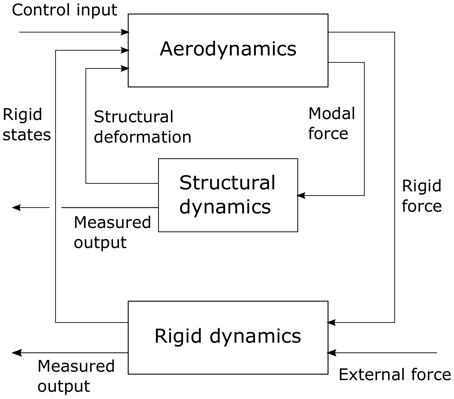
The nonlinear system of a flexible aircraft, which is developed using an approach based on subsystem modeling is shown in Figure 5. Aerodynamics, structural dynamics and rigid body dynamics are constructed separately and are built into a larger system to model motion and deformation of the aircraft. This is the ASE model. Different subsystems are modeled separately allowing various modeling techniques to be applied for each of them. Another advantage to this approach is its extendability, which means that additional subsystems can be included, for instance actuator or sensor dynamics, to create a more accurate ASE model.

Two dynamic aircraft models are constructed. One of them incorporates the aircraft dynamics with the rigid-, and the other with the flexible set of wings. The aerodynamic coefficients and derivatives are computed using XFLR5 software, an open-source design and analysis tool for airfoils, wings and planes [40]. The program currently allows airfoil, wing, winglet, horizontal and vertical stabilizer, control surface and fuselage design and analysis with the application of nonlinear lifting line theory (LLT), vortex lattice method (VLM) and a combined model of uniform source and doublet for thick bodies and horseshoe vortices for thin surfaces referred to as 3D Panel Method. To model the flexible wings, two MATLAB toolboxes that were created by the UMN research group were used [34]. These are the DLMTools toolbox for computing unsteady aerodynamics and FEMCode toolbox for elastic structural dynamics. Extensive description of the rigid and flexible models can be found in References [24,41].

4.1. Aircraft Model with the Rigid Set of Wings

The rigid model consists of two subsystems. One contains rigid-body equations of motion as presented in Reference [42] and the other calculates rigid body forces and moments. The latter uses aerodynamic coefficients computed using XFLR-5 software that were previously run based on Reference [40]. The XFLR-5 model of the aircraft was created with the ambition to gain the aerodynamic and stability properties and control parameters of the rigid version of the aircraft, and to determine the maximum hinge moments acting on the control surfaces. The original airfoil from the BFF aircraft is used on the aircraft’s entire span to create the model. For most of the aircraft’s original geometry this is an accurate approach, the only exception is the centerline of the body and its surroundings, where the landing skid, the GPS hood and the motor mount are located. However, these are neglected in the model to make the construction and later modifications less complicated. Control surface geometries are simplified for the same reason. Since the model is built up of cross-sections, the only way to model the flaps is in a streamwise sense, parallel to the cross-sections. The wingtip fences attached to the end of the wings make the construction of the plane using a single wing impossible. As a solution to this problem double fins are connected to the wingtips. As for mass properties, the total weight of the aircraft is defined in point masses representing the weight of built-in instruments and the structural mass of the aircraft. The instruments’ masses are placed at their exact location and the structural weight at the center of mass of each plane section described by its density.

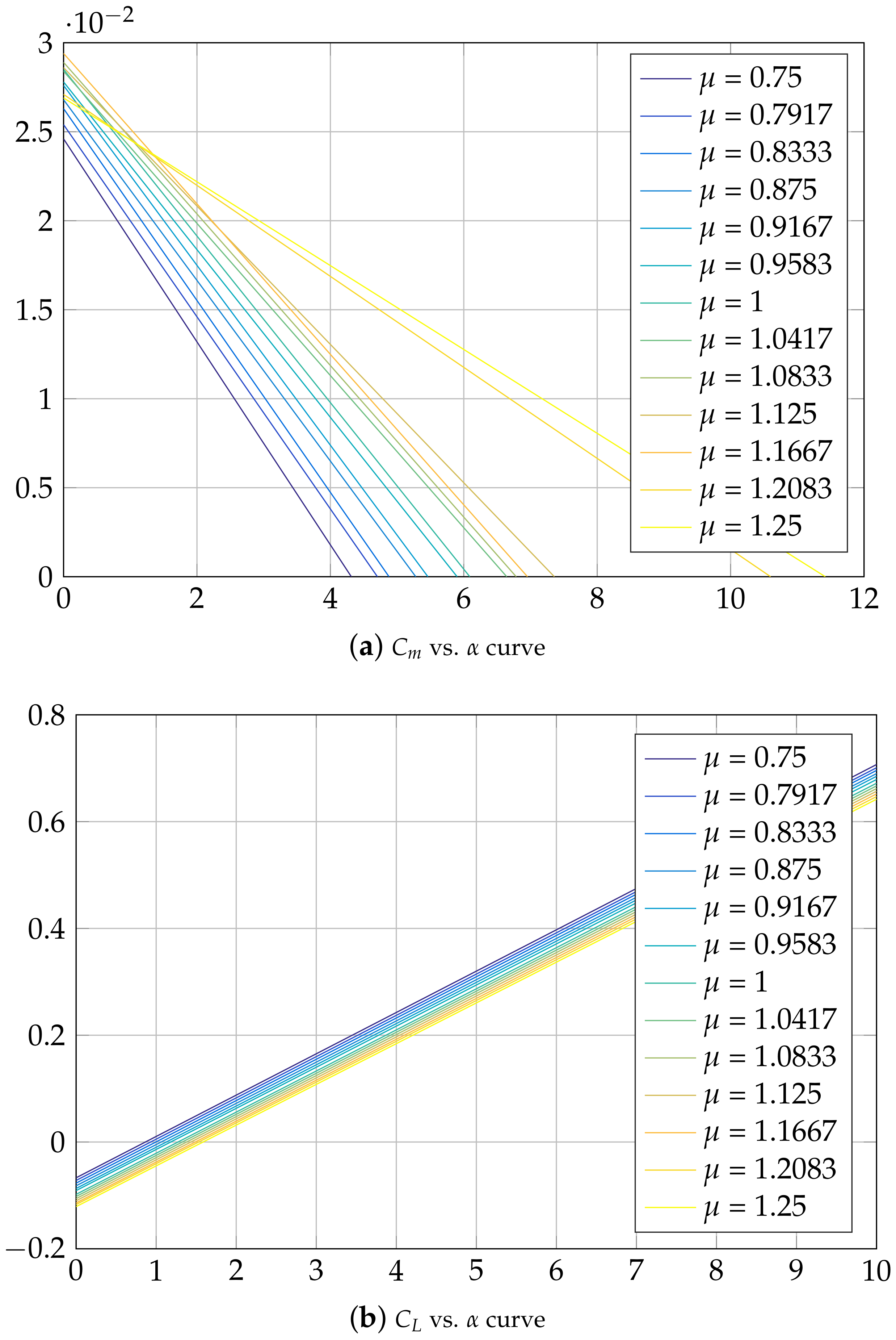
Based on the XFLR-5 software results, all 13 parametric versions of the rigid aircraft model can be obtained. The XFLR-5 software was also used to calculate the torques the actuators need to develop. The minimal actuator weights were then obtained from servo drive catalogs. To be able to build parameterized versions of the rigid body model, stability and control derivatives are also required for each control surface setup. Derivation of these coefficients is performed using the XFLR-5 software. After creating the models, stability analysis is run on each one to determine the desired values. Due to the modification of several equipment weights, the CG varies from model to model. This causes further differences in stability properties, which have to be considered at the evaluation and comparison of the models. The negative slope of the $C_m-\alpha$ curves in Figure 6. shows that each model is statically stable.

Figure 7 and Figure 8 show that the resulting aerodynamic coefficients require curve fitting in order to achieve model parameters between which interpolation is possible.

4.2. Aircraft Model with the Elastic Set of Wings

Structural vibration modes have a much greater effect on the dynamics of a flexible aircraft compared to a rigid vehicle. For this reason, modification of the previously described model is necessary to create an aeroelastic aircraft representation. For the flexible version a structural dynamics block is added and the aerodynamic model incorporates the unsteady dynamics of the flexible aircraft as well. In this case the mean axes reference frame serves as the base of the nonlinear equations of motion [43]. The mean axes frame is a convenient frame for modeling flexible aircraft. In addition to decoupling rigid body modes and vibrational modes, restriction of coupling to external forces and moments, as well as the satisfaction of translational and rotational mean axes constraints [43] are ensured. The nonlinear equations of motion in the previously introduced reference frame simplify as

$$\left[\begin{array}{cc}mI& 0\\ 0& J_{\mathrm{rig}}\end{array}\right]\left[\begin{array}{c}\dot{V_{\mathrm{r}}}\\ \dot{{\Omega }_{\mathrm{r}}}\end{array}\right]+\left[\begin{array}{c}mI{\Omega }_{\mathrm{r}}\times V_{\mathrm{r}}\\ {\Omega }_{\mathrm{r}}\times J_{\mathrm{rig}}{\Omega }_{\mathrm{r}}\end{array}\right]=\left[\begin{array}{c}\sum F_i\\ \sum M_i\end{array}\right],$$

(1)

where m is the mass, $J_{\mathrm{rig}}$ is the rigid inertia of the aircraft, $V_{\mathrm{r}}$ represents the translational velocity and ${\Omega }_{\mathrm{r}}$ the angular velocity with respect to inertial axes and $F_i$ and $M_i$ represent the forces and moments in the mean axes frame.

4.2.1. Structural Dynamics Model

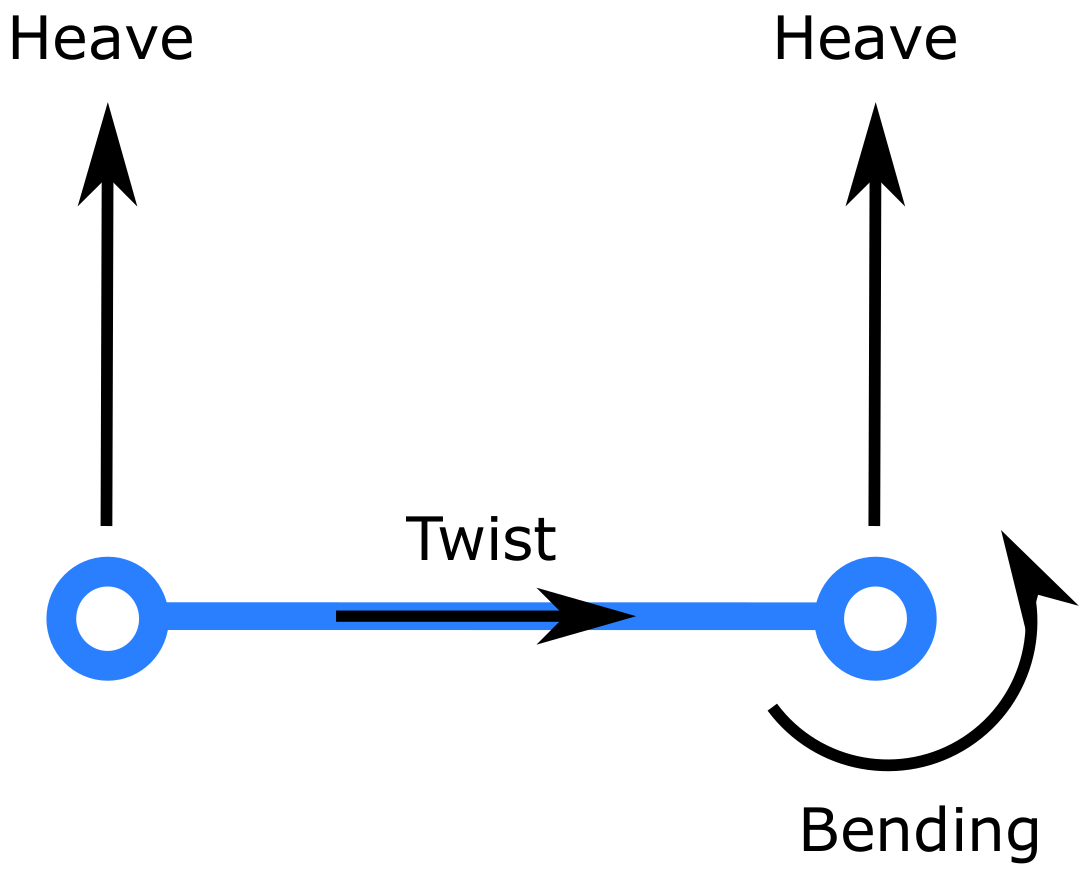
The structural model of the vehicle is created using the finite element method (FEM). The structure is discretized with respect to the vehicle’s physical characteristics, including for instance the location of control surface actuators, winglets and electronic components. The result of this discretization is a set of nodes connected by beams representing the structure of the aircraft. There are several types of beams available for flexible aircraft modeling, for example the chosen and commonly used Euler-Bernoulli beam with additional torsional effects (see Figure 9). The beams are connected with nodes that have 3 degrees of freedom, namely heaving, twisting and bending. The beam model was chosen since it directly models the structural mode of interest—symmetric wing bending—without having to model additional degrees of freedom. The BFF aircraft is not a hollow structure; it has ribs and spars that need to be modeled. Therefore, a shell structure is not truly representative of it. In summary, a beam model is more representative of the spar-rib structure of the actual vehicle, and it reduces the number of DoF required to model the structure compared to shell elements.

The structural model can be described with respect to modal coordinates as

$$M\ddot{\eta }+K\dot{\eta }+D\eta =F,$$

(2)

where M is referred to as the modal mass matrix, matrix K is called the modal stiffness matrix and D represents the modal damping matrix. $\eta$ is the modal coordinate describing the systems motion and F contains the external forces at all nodes. The generation of this model is done by applying the FEMCode Matlab toolbox [34]. The FEM model of the mini MUTT aircraft is presented in Figure 10.

This discretization results in a representation containing 14 nodes with 16 beams connecting them. This model introduces 24 states to the calculations, specifically the 12 modal coordinates and their derivatives. The natural frequencies and mode shapes resulting from the finite element calculations are summarized in

Table 2. Natural frequencies from the finite element model ($\mu =1$).

Mode Shape	Frequency [rad/s]
1st Symmetric Bending	34.90
1st Anti-Symmetric Bending	53.27
1st Symmetric Torsion	108.82
1st Anti-Symmetric Torsion	106.5532
2nd Symmetric Bending	163.20
2nd Anti-Symmetric Bending	183.64

[24].

The parameterization of the structural model is done by changing the actuator weights for each $\mu$ parameter. This creates a different mass matrix for each model. The first symmetric bending mode with respect to $\mu$ is presented in Figure 11. The natural frequencies and the mode shapes of the parameterized structural model vary only slightly with $\mu$. This is also expected, since the FEM model is not changed much. On the other hand, this is also beneficial because it can be expected that the flutter characteristics will not be altered significantly.

4.2.2. Unsteady Aerodynamics Model

Unsteady aerodynamics is modeled using the subsonic doublet lattice method (DLM [44]) while applying the solution of VLM for steady flow obtained at zero oscillating frequency. Both methods are potential-based panel methods, requiring the lifting surface to be separated into a grid of panels presented in Figure 12. According to Reference [45], the basic concept of panel methods is that a large number of elementary quadrilateral panels are placed on the actual or mean surface of the geometry in question. Each panel has one or more types of singularities attached to it, for instance sources, vortices or doublets. A functional variation across the panel can be specified to determine the singularities, for which the actual value is scaled by the corresponding strength parameters. The parameters can be calculated by solving the fitting boundary condition equations. The DLMtools toolbox from Reference [34] was used to obtain the parameterized unsteady aerodynamic models. In the following, the key aspects of the aerodynamic model is presented, further details can be found in References [24,39,46,47].

The key aspect of DLM, calculating unsteady frequency response, is that it assumes harmonic oscillations to occur in the flow around a fixed lifting surface. DLM does not differentiate between this occurrence and the case when a flexible wing oscillates harmonically in steady flow. The method provides an aerodynamic model in frequency domain, with the angle of attack distribution of the wing as an input and the derived pressure distribution on the lifting surface calculated from the normalwash distribution as an output. There is no such constraint in this method that the lifting surface must be rigid, as each panel is assumed to move individually, which means it is applicable for flexible aircraft as well. The normalwash vector $\overline{w}$ in (3) can be calculated if elastic deformation of the surface can be approximated in terms of panel motion. Thus using DLM, the pressure distribution of the wing can be obtained. The DLMTools toolbox generates the Aerodynamic Influence Coefficient ($AIC$) matrix for the given aerodynamic grid. From this the pressure distribution $\overline{p}$ is calculated as

$$\overline{p}=\left[AIC(\omega ,V)\right]\overline{w}.$$

(3)

where $\omega$ is the oscillating frequency, V is the airspeed and $\overline{w}$ is the normalwash vector. The oscillating frequency and flow speed can be combined in a dimensionless parameter, as:

$$k={\displaystyle \frac{\omega \overline{c}}{2V}}.$$

(4)

where k is the reduce frequency and $\overline{c}$ is the reference chord of the lifting surface. The aerodynamic forces and moments are calculated from the pressure distribution using the obtained $AIC\left(k\right)$ matrix as

$$F_{aero}=\overline{q}{S}_p\left[AIC\left(k\right)\right]\overline{w},$$

(5)

where $\overline{q}$ is the free stream dynamic pressure and $S_p$ is the panel area matrix.

It is important to mention however that an additional method called surface spline theory is introduced to project modal displacement on the aerodynamic grid. This method is capable of interpolation between a given set of deformation using thin plate deformation equations, which means that it is able solve for the unknown deformation of any point situated on the given surface. The purpose of its application is to transform all degrees of freedom of the nodes of the structural grid purely to heaving motion of the nodes of the spline grid. Prior to the interpolation, the structural deformations need to be represented on an infinite thin plate. Deformation of such plates is only possible in the direction normal to their surface, so modal displacements have to be expressed in terms of heave exclusively. This can be achieved by applying the so called spline grid, which is presented for the Mini MUTT in Figure 13. The spline grid is generated based on the previously assembled structural grid.

Since the structural model is given in generalized modal coordinates, transformation of the aerodynamic load to a coordinate system that is compatible with the structural model is necessary. To map modal deflection to the resulting aerodynamic load, a matrix called the Generalized Aerodynamics Matrix (GAM) has to be obtained. The resulting GAM matrices are obtained in frequency domain. However, time domain aeroelastic simulations require a continuous model. To achieve the continuous model, Roger’s rational function approximation (RFA) [48] is applied [32,46]. Using RFA, additional lag states are introduced representing the lag behaviour of the aerodynamic model. Aerodynamic lag terms can be defined in the following state-space form

$$\begin{array}{cc}\hfill {\dot{x}}_{aero}& =\frac{2V}{\overline{c}}{A}_{lag}{x}_{aero}+B_{lag}{\left[\begin{array}{ccc}{\dot{x}}_{rigid}& \dot{\eta }& \dot{u}\end{array}\right]}^T\hfill \\ \hfill y_{aero}& =C_{lag}{x}_{aero}.\hfill \end{array}$$

(6)

In addition, since the resulting aircraft representation only accounts for three force and moment components, the remaining components can be obtained by computing rigid body forces and moments, for example.

In the current case, modification of the aerodynamic grid parameterizes the unsteady aerodynamics model. This is done using $\mu$ values to match the length of flaps to the different versions of the model. In the original version control surface chords are divided into three even parts. According to the thumb rules for grid setup presented in Reference [49], the chosen $\mu$ values do not allow change in the number of chordwise divisions of either the wing or the flaps. This is due to the resulting overly high panel aspect ratios or too low values for chordwise divisions. The GAM matrices of the aerodynamics are generated based on the resulting grid data.

Using the structural dynamics data coming from the FEMcode, the unsteady aerodynamics data from DLMtools, the missing aerodynamic coefficients from the XFLR-5 software and the mean axis approach, nonlinear parametric aeroelastic model of the mini MUTT model can be constructed.

5. LPV Modeling of the Mini MUTT Aircraft

The mini MUTT models obtained in the previous section are nonlinear. However, control design for nonlinear systems is a challenging task and in general controllers are usually synthesized based on a simpler representation of the system. The paper focuses on LPV system representation. LPV systems [16,17] are linear systems, whose state-space models are known functions of time-varying parameters. The time variation of each of the parameters is not known a priori, but is assumed to be measurable in real-time. LPV system representations are well suited for aerospace applications [50].

5.1. LPV Modeling

An LPV system is described by the state space model

$$\begin{array}{cc}\hfill & \dot{x}\left(t\right)=A\left(\rho \left(t\right)\right)x\left(t\right)+B\left(\rho \left(t\right)\right)u\left(t\right)\hfill \\ \hfill & y\left(t\right)=C\left(\rho \right(t\left)\right)x\left(t\right)+D\left(\rho \right(t\left)\right)u\left(t\right)\hfill \end{array}$$

(7)

with the continuous matrix functions $A:\mathcal{P}\to {\mathbb{R}}^x$, $B:\mathcal{P}\to {\mathbb{R}}^x$, $C:\mathcal{P}\to {\mathbb{R}}^x$, $C:\mathcal{P}\to {\mathbb{R}}^x$, the state $x:\mathbb{R}\to \mathbb{R}$, input $u:\mathbb{R}\to \mathbb{R}$, output $y:\mathbb{R}\to \mathbb{R}$ and a time-varying scheduling signal $\rho :\mathbb{R}\to \mathcal{P}$, where $\mathcal{P}$ is a compact subset of ${\mathbb{R}}^{\rho }$. Elements of the state vector x may be included in the parameter vector $\rho$. In that case the system is called a quasi LPV model.

Different types of representations are available for LPV systems, including grid-based [15,18,51], linear fractional transformation (LFT) [19,20,51] and polytopic [21,52] approaches. The present work focuses on grid and a polytopic LPV model representations.

5.2. Grid-Based LPV Representation

A grid representation consists of a series of Linear Time-Invariant (LTI) models generated by evaluating the LPV model at a range of parameter values ${{\rho }_k}_1^{N_{g}rid}={\mathcal{P}}_{g}rid\in \mathcal{P}$. The resulting system matrices are $(A_k,B_k,C_k,D_k)=(A\left({\rho }_k\right),B\left({\rho }_k\right),C\left({\rho }_k\right),D\left({\rho }_k\right))$. A typical grid-based LPV model of an aircraft is shown in Figure 14.

In the grid-based approach the system is stored as a finite state-space array. Grid points correspond to LTI models, which describe the dynamics of the system when the parameter(s) of the grid point is held constant. To compute a sufficiently accurate model the grid must be dense enough, which can make this approach less efficient computationally.

5.3. TP Type Polytopic LPV Representation

An overview of the polytopic representation is presented here, taken from more detailed descriptions including References [21,22] In the present case the grid based LPV model serves as a base for tensor produc (TP) model transformation [22]. Let the system matrix be written as

$$S\left(\rho \left(t\right)\right)=\left(\begin{array}{c}A\left(\rho \right(t\left)\right)B\left(\rho \right(t\left)\right)\\ C\left(\rho \right(t\left)\right)D\left(\rho \right(t\left)\right)\end{array}\right).$$

(8)

Time dependence t is suppressed occasionally in the remainder of this paper in order to shorten the notation. In addition, different control performance requirements represented by parameter dependent channels can be incorporated into $S\left(\rho \right)$.

The system matrix $S\left(\rho \right)$ of (8) can be converted for any parameter $\rho$ into the following polytopic form:

$$S\left(\rho \right)=\sum _{r=1}^R{w}_r\left(\rho \right)S_r.$$

(9)

The ordering $r=ordering(i_1,i_2,\dots i_n,i_{n+1},\dots i_N)$, determines r as a linear index. It is a multilinear array index with the size $I_1\times I_2\dots I_{n-1}\times I_{n+1}\dots I_N$, $w_r\left(\rho \right)={\prod }_{n=1}^N{w}_{n,i_n}\left({\rho }_n\left(t\right)\right)$ and $S_r=S_{i_1,\dots ,i_N}$. The polytopic TP model form of (9) based on the canonical higher order singular value decomposition (HOSVD) consists of [53,54,55]:

$$\begin{array}{cc}\hfill S\left(\rho \right)& =\sum _{i_1=1}^{I_1}\cdots \sum _{i_N=1}^{I_N}\prod _{n=1}^N{w}_{n,i_n}\left({\rho }_n\right)S_{i_1,\dots ,i_N},\hfill \end{array}$$

(10)

which consists of weighting functions $w_n\left({\rho }_n\left(t\right)\right)$ and the, singular value ordered, parameter-varying orthonormal combination of LTI matrices $S\in {\mathbb{R}}^{O\times I}$. These LTI systems are termed vertex systems. Applying the compact tensor notation leads to the canonical TP type polytopic model that is based on HOSVD:

$$\begin{array}{cc}\hfill S\left(\rho \right)& =\mathcal{S}\underset{n\in N}{⊠}{w}_n\left({\rho }_n\right).\hfill \end{array}$$

(11)

In this representation the core tensor’s coefficients $\mathcal{S}\in {\mathbb{R}}^{I_1\times \dots \times I_N\times O\times I}$ are obtained from the LTI vertex matrices $S_{i_1,\dots ,i_N}$, row vectors $w_n\left({\rho }_n\right)$ from the univariate weighting functions $w_{n,i_n}\left({\rho }_n\right)$, $i_n=1\dots I_N$ and ${\rho }_n$ that consists of the n-th element of vector $\rho$.

Finally, the qLPV model in TP structure is defined as:

$$\left[\begin{array}{c}\dot{x}\\ y\end{array}\right]=\mathcal{S}\underset{n\in \mathrm{N}}{⊠}{w}_n\left({\rho }_n\right)\left[\begin{array}{c}x\\ u\end{array}\right].$$

(12)

The $N+2$-dimensional core tensor $\mathcal{S}\in {\mathbb{R}}^{I_1\times \cdots \times I_N\times O\times I}$ is generated using the LTI system matrices $S_{i_1,\dots ,i_N}\in {\mathbb{R}}^{O\times I}$. If the vertex systems define a convex combination of the weighting functions for all n, then

$$\left[\begin{array}{c}\dot{x}\\ y\end{array}\right]=\mathcal{S}\underset{n\in \mathrm{N}}{⊠}{w}_n^{Co}\left({\rho }_n\right)\left[\begin{array}{c}x\\ u\end{array}\right]$$

(13)

and the TP model consists of a polytopic form. In thus case $S\left(\rho \right)$ system matrix is always within $co\{\forall n,i_n:S_{i_1,\dots ,i_N}\}$, where the LTI systems $S_{i_1,\dots ,i_N}$ are the vertices of the polytope. The polytopic TP model can be always converted to general polytopic model as:

$$S\left(\rho \right)=\sum _{r=1}^R{w}_r^{Co}\left(\rho \right)S_r.$$

(14)

Therefore, it can be considered as a higher structured polytopic representation.

Vertexes $S_r$ are identical to the vertexes contained in tensor $\mathcal{S}$, as $S_r=S_{i_1,i_2,\dots ,i_n}$ and $w_r\left(\rho \right)={\Pi }_{n=1}^N{w}_{n,i_n}\left({\rho }_n\right)$. The finite index r is a linear version of multidimensional indexes $i_1,i_2,\dots ,i_N$.

In case the weighting functions $w_n\left({\rho }_n\right)$, $Co$ satisfy

$$\forall n,{\rho }_n:w_n\left({\rho }_n\right)=1$$

(15)

$$\forall n,i,{\rho }_n:w_{n,i}\left({\rho }_n\right)\in [0,1]$$

(16)

the polytopic TP model (12) is convex. The convex weighting functions in this case are denoted as $w_n^{Co}\left(x_n\right)$. There are many convex TP model representations available [52,56]. The current paper focuses on the Close to Normal (CNO) type TP model is a Normal (NO) type model. In this case the weighting functions satisfy (15) and (16) and in addition, 1 or a value close to 1 is the largest value of all weighting functions for each dimension n.

5.4. Grid-Based LPV Model of the Mini MUTT Aircraft

LPV models of the mini MUTT aircraft model can be achieved in the same way for the rigid and flexible wing model as well. To keep the paper concise, the flexible wing set model will be the focus for the remainder of the paper. The grid-based LPV model can be generated for the Mini MUTT model by Jacobian linearization as presented in Reference [57]. Trimming of the aircraft dynamics is executed assuming straight and level flight condition at the range of airspeed $V=\left[20,33\right]$ m/s at 66 equidistant points. Thus the airspeed becomes the scheduling parameter $\rho$. The second dimension of the scheduling parameters is $\mu$. The model developed is a quasi-LPV system [32], because $\rho$ depends on rigid body velocities u, v and w. The pole migration of the nominal LPV model ($\mu =1$) is given in Figure 15. The pole migrations and the flutter speeds have only a very minor change with respect to $\mu$, thus the $\mu$ variations are not shown in the plot. The plot, for better visibility, does not show the actuator dynamics and high frequency aeroelastic modes. It can be observed how the flutter mode goes unstable as the airspeed increases.

6. Bottom-Up Modeling of the Mini MUTT Aircraft

The parametric LPV model of the aircraft with the flexible wing set, obtained in the previous section, has 12 elastic modes and 52 aerodynamic lag states. Combined with the rigid body states and the actuator dynamics the ASE model consists of 104 states. Let us denote this model as a high fidelity model. Such high order LPV model is unsuitable for control synthesis. Either LPV model order reduction techniques [26,27,28,29,30,31], or a bottom-up modeling approach can be applied as presented in Reference [32] to obtain a control oriented, reduced-order model. The present paper focuses on the latter. The key idea of the bottom-up modeling is the following: structural dynamics and aerodynamics are modeled in subsystems based on FEM and DLM. When combined, these subsystems provide a simpler model structure compared to that of an overall ASE model. Moreover, the reduction of the individual subsystems is a much more straightforward task for which more tractable reduction techniques can be employed. The key aspect of low order subsystems is that the aircraft’s actuator bandwidth determines whether a given mode is effectively controllable or not. In the case of the Mini MUTT flutter occurs around 30 rad/s and the bandwidth of the servo is approximately 133 rad/s. Here, the frequency region of interest can be limited to 100 rad/s in which we expect the control oriented bottom-up model to match the high fidelity model accurately.

The parameterized structural model, obtained in Section 4.2.1, only needs to the modes lying within the actuator bandwidth. The structural dynamics model is therefore reduced by retaining the first 4 structural modes. The remaining 8 modes are truncated and structural dynamics is represented with 8 states, ${\eta }_{1\cdots 4}$ and ${\dot{\eta }}_{1\cdots 4}$.

The AIC matrices obtained in Section 4.2.2 are used for the bottom-up model. However, in this case the $GAM$ matrices are generated only for the remaining 4 elastic modes. This results in an unsteady aerodynamics model with 36 lag states. A linear balancing transformation matrix T is then computed for the aerodynamics model given by $A_{la{g}_{}}$, $B_{la{g}_{}}$ and $C_{la{g}_{}}$ in (6). The reduced order aerodynamics model is obtained by rezidualizing the states with the smallest Hankel singular values. The reduced aerodynamics model is obtained by retaining 4 lag states.

The nonlinear, parameterized control oriented ASE model can then be built using these reduced subsystems. The resulting control oriented ASE model contains 40 states.

6.1. Assessment of the Control Oriented Parametric Model

It is crucial to verify if the control oriented 40 state model is a good approximation of the high fidelity 104 state model. Several options are available for such evaluation including the $\nu$-gap metrics [26] examination, frequency response comparison, and so forth [32,58]. The first step of the assessment is to obtain a grid-based LPV model of the control oriented model as for the high fidelity, 104 state model. The $\nu$-gap metric can be used to compare the original full-order and the bottom-up model of the aircraft. The $\nu$-gap metric ${\delta }_{\nu }(\dot{;}\dot{)}$ is chosen to be used as a measure, since it takes the feedback control objective into account. The $\nu$-gap takes values between zero and one. If the value is zero, the two systems are identical. A system $P_1$ that is within a distance $ϵ$ to another system $P_2$ in the $\nu$-gap metric, that is, ${\delta }_{\nu }(P_1;P_2)<ϵ$, will be stabilized by any feedback controller that stabilizes $P_2$ with a stability margin of at least $ϵ$ [59]. A plant at a distance greater than $ϵ$ from the $P_2$, however, will in general not be stabilized by the same controller. This means that the $\nu$-gap metric approximates whether a feedback controller designed for the lower order model will be efficient on the full order model. The $\nu$-gap values are shown in Figure 16. The $\nu$-gap values remain around 0.1 for up to 90 rad/s frequency and rapid growth does not occur within the frequency range defined by the actuators. Consequently, the low order LPV model is sufficiently accurate inside the frequency range of interest.

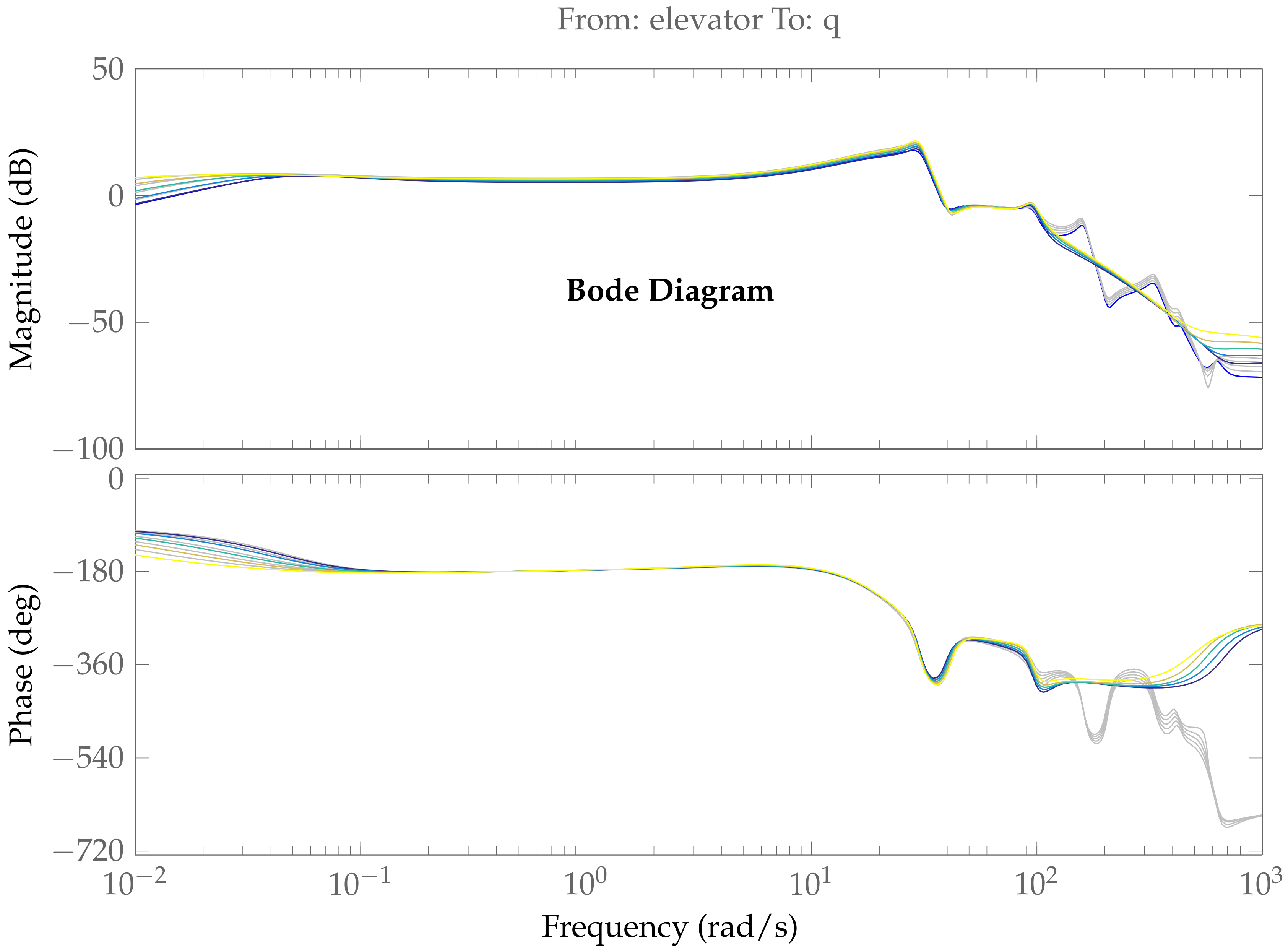
In addition to the $\nu$-gap values, the bode plots of 40 and 104 state models are compared in Figure 17 and Figure 18. In these figures the colors represent the $\mu$ parameters of the control oriented model, while the grey plots are of the full order model. It can be also observed that the bode plots match very well within the frequency range of interest.

6.2. Polytopic Model of the Control Oriented Mini MUTT Aircraft

The previously obtained control oriented, grid based LPV model serves as the base of the TP model transformation. The grid upon which the TP model transformation is carried out is of the dimension $66\times 13$. These are, the airspeed and the $\mu$ values. TP model transformation results in 3 dominant singular values in the airspeed dimension and 2 dominant singular values in the $\mu$ dimension as

$$\left[\begin{array}{c}43900.138\\ 1347.518\\ 33.851\end{array}\right],\left[\begin{array}{c}397728.24\\ 5289.531\end{array}\right].$$

Retaining these singular values, a polytopic model with $3\times 2$ vertex systems is obtained. Note, that since nonzero singular values were discarded, this is only an approximated model of the original grid-based LPV system.

In order to obtain a convex polytopic model, CNO type weighting functions are derived. The weighting functions for the CNO type convex model is given in Figure 19. Note, that the CNO type representation introduced an additional vertex system in the $\mu$ dimension. The convex vertexes are given with system matrices $S^{68\times 43\times 3\times 3}$. It can be observed from the weighting functions that reduction of the number of models is possible when considering airspeed as well as the $\mu$ value. In case of the airspeed, 3 vertex systems are sufficient instead of the original 66 grid points, whereas in the $\mu$ dimension the number of grids were reduced from 13 to 3.

7. Conclusions

Parametric aeroservoelastic models of the mini MUTT aircraft suitable for co-design have been developed. Both, rigid and flexible wing models are obtained. Low order, control oriented LPV models were derived using the bottom-up modeling approach. With this approach the number of states were reduced from 104 to 40 while retaining the physical meaning the states. The $\nu$-gap metric and bode plots show that the control oriented model is accurate within the frequency range of interest. The resulting models show enough variations for the simultaneous control surface sizing and control synthesis optimization tasks, while not altering significantly the flutter characteristics. Both grid and polytopic models were derived. The polytopic models are derived based on TP model transformation. It was possible to significantly reduce the number of vertex systems for the polytopic model, from $66\times 13$ to $3\times 3$. Using the grid and polytopic models, different control design methodologies can be applied for co-design.