Feeding of Plankton in a Turbulent Environment: A Comparison of Analytical and Observational Results Covering Also Strong Turbulence

Abstract

The present studies address feeding of plankton in turbulent environments, discussed by a comparison of analytical results and field data. Various models for predator-prey encounters and capture probabilities are reviewed. Generalized forms for encounter rates and capture probabilities in turbulent environments are proposed. The analysis emphasizes ambush predators, exemplified by cod larvae Gadus morhua L. in the start-feeding phase (stage 7 larvae) collected in shallow waters near Lofoten, Norway. During this campaign, data were obtained at four sites with strongly turbulent conditions induced by tidal currents and long-wave swells, and one site where the turbulence had a lower level in comparison. The guts of the selected cod larvae were examined in order to determine the number of nauplii ingested. Analytically obtained probability densities for the gut content were compared with observations and the results used for estimating the rate of capture of the nauplii. This capture rate was then compared with analytical results using also data for the surroundings, such as measured prey densities and turbulence conditions, as quantified by the specific energy dissipation rate. Different from earlier studies, the presented data include conditions where the turbulence exceeds the level for optimal larval encounter-capture rates.

1. Introduction

The survival rates of fish in their early life-stages are influenced by a number of biological and physical processes [1,2]. A number of models have been proposed for several individual partial processes. Models for predator-prey encounter rates, in particular, form the basis of many biological applications, including the feeding rates of larval fish and the implications of environmental effects on their growth and survival [3,4]. Pioneering studies [5,6] argued that turbulent motions in the local environment could be important by enhancing encounter rates between predators and prey. Prior to these studies, turbulence was assumed to reduce predator-prey encounter rates because of the effect of prey dilution and breaking down the peak concentrations. The question was how known physical laws for turbulence modeling, such as the Kolmogorov-Obukhov law for the second order structure function, are reflected in the predator-prey encounter rate. Many elements of various models have been tested under controlled laboratory conditions using small polystyrene particles as representing plankton [7,8]. The turbulence conditions could be varied systematically by controlling the external stirring mechanism that created the turbulence. Models were tested also by numerical simulations where plankton was represented by point particles passively following the turbulent motions in the flow [9,10]. Studies allowing for self-induced motions have also been presented [11,12]. It was, however, realized that too strong turbulence could have an adverse effect for the predator by reducing the capture probability of prey [13,14,15]. Low turbulence levels give an advantage by increasing the encounter rate, while too strong turbulence can be disadvantageous by reducing the capture rate to such an extent that it partially dominates the effect of turbulent encounters. The result is the existence of an optimum turbulence level that is a characteristic for the given species. A dome-shaped relationship for the predator capture rate as a function of turbulence intensity $ϵ$ has been suggested based on predator response time and and reactive distance [13]. The present study outlines the properties of various models for the encounter rate in turbulent environments and includes also the consequences of the reduce capture rate for large turbulence levels. For ambush predators we assume that the encounter and capture rates are basically controlled by turbulent motions in the environment. For the capture they can rely on both visual identification and organs sensing disturbances in the water [16,17].

In the present study we compare analytical results with results obtained by analyzing field data of the gut content of fish larvae collected in the shallow waters near Lofoten, Norway. Additional material is presented elsewhere [18]. Predators (in the present case cod larvae, Gadus morhua L.) were sampled by two different methods: 1) an ichthyoplankton net moved slowly from the seabed to the surface, thereby vertically integrating the larval samples, and 2) a high-capacity submersible pump (HUFSA) at selected positions 5, 10, 15, 20, 25 and 30 m below the surface. The guts of the selected larvae were opened under a microscope and a database established for the number of nauplii in the guts, together with the length of the corresponding cod larvae. The entire database consists here of 3247 entries, containing the simultaneously obtained lengths and gut contents of cod larvae supported by the experimentally determined local specific energy dissipation rate $ϵ$. The data obtained by the pump are depth resolved, with corresponding local prey concentrations. The subset collected by the net is an average over all depths, and this part of the database contains 866 entries. Cruising speeds of cod larvae as observed during laboratory conditions are in the velocity range 0.1–0.3 mm s${}^{-1}$ [19]. This can be approximately one order of magnitude higher cruising speed than that of their naupliar prey [20]. We do not expect any significant differences between the two datasets as far the vertical distribution is concerned. For a small subset consisting of 299 samples evenly distributed over depth, also the lengths of the nauplii found in the guts were measured. The ambient concentrations of the nauplii (prey) were sampled by a zooplankton pump at discrete depth positions. The details of the biological sampling in the field and the processing of the samples in the laboratory is similar to two other studies [21,22]. These studies deduced the cod larval ambient turbulence energy dissipation rate of the mixed layer from averaged wind-induced turbulence based on the empirical results [23]. The present study, on the other hand, calculated the turbulent energy dissipation rate $ϵ$ by measuring the turbulence using acoustic current meters from a point observation at the top of a 6.5 m high tower, deployed on the seabed at the shallow observation sites.

The database obtained on the basis of the field data were used for a test of analytical predictions. Analytical models for probability densities for the gut content were thus compared with observations to give an estimate of the rate of capture of the nauplii. This capture rate was then compared with analytical results.

2. Results

The present study contains two parts, analytical results and study of data from a field experiment, where the data could be analyzed to give a form amenable for comparison with theory. The present section is divided into two parts addressing these two approaches separately.

2.1. Analytical Results

The present analytical part will mostly be a review of some of the existing models for predator-prey encounter rates and capture probabilities in turbulent environments. The discussion is separated into two parts.

2.1.1. Encounter Rates in Turbulent Flows

To illustrate the complexity of the problem of particle moving in a turbulent flow we show Figure 1 and Figure 2. The two figures allow a three-dimensional, stereoscopic view. It requires a little exercise. The observer should focus the eyes approximately 20 cm behind the plane of the paper or computer screen. The distance to the eyes is not so critical provided it is sufficiently large, but it is essential that the figure is kept plane and horizontally aligned with the observers eyes. Figure 1 shows a group of point particles moving in a turbulent flow; one of the particles indicated by red color represents the predator, and the others a group of prey that happened to be close to it at some initial time. The presentation is given in the fixed laboratory, or Eulerian, frame. At first sight, the motion does not seem to be particularly complicated; the particles move like a group with some small relative motion. The problem is that the figure is shown in the wrong frame of reference. The correct frame for the present problem is the Lagrangian frame, one that moves with the predator. This is shown in Figure 2 and here the relative motions are much more complicated. A complete detailed analysis of the motion of the particles is not possible, and only a statistical analysis is feasible. The desired results should account for the average flux of particles presenting prey through a given surface (not necessarily spherical) that represents the range of the predator. We associate a characteristic length $R_c$ with this range.

Depending on the parameters of the turbulence and the characteristics of the predator, we can envisage two limiting cases. One is where $R_c$ is in the inertial range of the turbulence, and one where it is in the viscous subrange. A dimensional analysis estimates the separation length as the Kolmogorov microscale $\eta ={({\nu }^3/ϵ)}^{1/4}$, where $\nu$ is the kinematic viscosity of the water [26]. A numerical coefficient can, however, not be determined by this argument, and it has to be found by other methods.

We consider the longitudinal velocity structure function $\langle {\left(u_{\Vert }(\mathbf{x},t)-u_{\Vert }(\mathbf{x}+\mathbf{r},t)\right)}^2\rangle /\sqrt{\nu ϵ}$, where the subscript ‖ indicates the velocity component in the direction along $\mathbf{r}$. The Kolmogorov velocity scale is $u_K={\left(\nu ϵ\right)}^{1/4}$. Two relevant subranges can be identified for the turbulent velocity fluctuations, (1) the inertial range with the Kolmogorov-Obukhov structure function $C_K{ϵ}^{2/3}{r}^{2/3}$ with $C_K\approx 2.0-2.5$ being an empirically determined numerical coefficient [27], and (2) the viscous subrange with a structure function $C_{\nu }{r}^2ϵ/\nu$, where a numerical coefficient $C_{\nu }=1/15$ is obtained analytically [28]. A modified Kolmogorov scale ${\eta }_0$ is defined as the scale separating these two universal subranges. It is readily determined as the length scale ${\eta }_0\equiv \eta {\left(15C_K\right)}^{3/4}$, where the values of the two structure functions are equal [10], see also Figure 3. We find ${\left(15C_K\right)}^{3/4}\approx 13$ so it is not a trivial correction factor.

In Figure 3 we show by a full continuous line a phenomenological interpolation function for the structure function covering both inertial and viscous subranges [29]. The analytical form is

$$St(r/\eta )=\frac{C_K{C}_{\nu }{(r/\eta )}^{8/3}}{C_{\nu }{(r/\eta )}^2+C_K{(r/\eta )}^{2/3}}.$$

(1)

With the given normalization used for the structure function in Figure 3, we find that $St(r/\eta )$ reproduces both the inertial and viscous subranges for large and small r, respectively.

The encounter rate (here denoted $J_e$) for point particles in turbulent flows have been investigated analytically by a significant number of studies, noting that relevant results, apart from a numerical constant, can be obtained with a relatively straight forward dimensional reasoning [8]. These idealized point-particles are then assumed to represent predators and prey. The accuracy of this assumption has been discussed [10], suggesting some improvements for the modeling on the expense of more complicated analytical expressions. The full analysis needs not be reproduced here since it is available in the literature, where also reviews can be found [30]. We have an expression for the turbulent encounter rate for predators moving like point particles surrounded by a spherical encounter surface with a radius $R_c$ in the inertial subrange. For this idealized case the expression

$$J_{e,I}=C_M{D}_0{ϵ}^{1/3}{R_c}^{7/3}$$

(2)

was found [29], with $C_M$ being a universal numerical coefficient. The expression (2) reproduces also previous results [6] for the ${ϵ}^{1/3}{R_c}^{7/3}$ scaling in the inertial subrange ${\eta }_0<R_c<L_E$, with $L_E$ being the outer scale limiting the inertial subrange. We introduced $D_0$ as the reference density (or concentration) of prey. In the limit $R_c>{\eta }_0$, it is possible to obtain analytical expressions [31] for the full time variation of the flux when the problem is solved for an initial condition with constant density for $r>R_c$. For spherical encounter surfaces with radius $R_c$ in the viscous subrange an expression in the form

$$J_{e,v}=C_{\nu }{D}_0{R_c}^3\sqrt{\frac{ϵ}{\nu }}$$

(3)

was found [29]. The expression (3) gives an ${R_c}^3\sqrt{ϵ/\nu }$ scaling of the turbulent flux for the viscous subrange $0<R_c<{\eta }_0$, with a numerical constant $C_{\nu }\ne C_M$. From experiments or numerical simulations, the numerical coefficients were determined empirically [29] to be $C_{\nu }\approx 1$ while $C_M\approx 6-7$. The dimensionless combination $D_0{R}_c^3$ gives (apart from a numerical constant) the number of prey within a spherical capture region and is a useful quantity for normalizations.

We found [10] an approximate simple empirical relation

$$J_e=C_A\frac{{ϵ}^{1/3}{D}_0{R}_c^3}{R_c^{2/3}+{\eta }_0^{2/3}},$$

(4)

which contains the parameter variation of the two limiting cases $R_c\ll {\eta }_0$ and $R_c\gg {\eta }_0$, as well as the correct cross-over length scale ${\eta }_0$. The effect of viscosity enters solely through ${\eta }_0$ in (4). Empirically, a coefficient $C_A\approx 7$ was found to give the numerical factors of the $J_e$-variations in the two relevant subranges correct within 15%. This result is consistent with numerical [10] as well as laboratory results [8]. The normalized expression $J_e/\left(D_0{R}_c^3\right)$ based on (4) which will be used later is ill posed in the limit of $R_c\to 0$, with a diverging derivative there. This singularity has no physical consequences. Even for relatively large radii, e.g., $R_c=10\eta$, we have contributions from viscosity, emphasizing that viscous effects can be more important than generally accepted for the present context. In Figure 4 we show (4) for varying $ϵ$ and $R_c$ in physical units taking ranges relevant for our database. We choose to normalize $J_e$ with $D_0{R}_c^3$ and a time scale $t_m$ that will be defined later. This normalization is natural here, but gives rise to a “hidden” dependence on $R_c^3$.

The assumption of a spherical encounter surface is usually considered to be an oversimplification. More realistic models take a conical surface [32,33,34] with some opening angle $\theta$, where hemispherical surfaces have often been assumed. There is empirical evidence that the results can be modified simply by introducing a multiplier for $J_e$ in terms of a correction factor $\chi \left(\theta \right)$ which has an empirical form [29] where $\chi \approx 1$ for $\theta >{100}^{\circ }$ while

$$\chi \left(\theta \right)\approx 0.31\theta +0.19{\theta }^2-0.06{\theta }^3,$$

(5)

with $\theta$ given in radians [29] for $0\le \theta <\pi /2$. The difference between $\chi \left(\theta \right)$ obtained for the viscous and inertial subranges is moderate [10], but in principle the ranges should be considered separately also in this respect.

The results quoted so far assumed both predators and prey to be passively following the turbulent motions in the flow. Self-induced motion patterns can also be taken into account by phenomenological models. For a simple cruising predator motion with prey passively following the flow, evidence was found [12] for a simple encounter rate expression in the form

$$J_e=\sqrt{J_0^2+{\left(D_0\pi R_c^2{V}_{c}h\left(\theta \right)\right)}^2},$$

(6)

where $V_c$ is the cruising velocity, assumed constant, while the factor accounting for the “clearing surface” is $h\left(\theta \right)={sin}^2\theta$ for $\theta <{90}^{\circ }$ and $h\left(\theta \right)=1$ for $\theta >{90}^{\circ }$. The notation $J_0$ indicates the turbulence-induced encounter rate experienced by a predator at rest, with a seemingly universally useful approximation given by (4). The cruising velocity is measured in the local fluid element, and the root-mean-square (RMS) fluid velocity in the Eulerian frame of reference is not relevant for comparison; the Kolmogorov velocity $u_K$ is more appropriate, see

Table 1. Summary table of field data and some quantities derived from them.

Station	$\langle {\mathit{L}}_{\mathit{\ell }}\rangle$ [mm]	$\langle {\mathit{N}}_{\mathit{H}}\rangle$	${\mathit{D}}_0$ [l${}^{-1}$]	$\langle \mathit{a}\rangle$ [$\mathsf{\mu }$m]	$\mathit{ϵ}$ [m${}^2$s${}^{-3}$]	${\mathit{\eta }}_0$ [mm]	${\mathit{\tau }}_{\mathit{K}}$ [s]	${\mathit{u}}_{\mathit{K}}$ [m s${}^{-1}$]
I	4.69	1.99	11.22	299	1.12$\times {10}^{-6}$	17.11	1.16	1.14$\times {10}^{-3}$
II	4.80	1.45	9.17	299	3.62$\times {10}^{-6}$	12.77	0.64	1.53$\times {10}^{-3}$
IIIA	4.72	2.09	19.74	245	5.44$\times {10}^{-5}$	6.49	0.17	3.01$\times {10}^{-3}$
IIIB	4.70	1.62	13.59	306	1.70$\times {10}^{-5}$	8.68	0.30	2.24$\times {10}^{-3}$
IV	4.22	3.34	7.90	214	4.25$\times {10}^{-8}$	38.80	5.94	5.03$\times {10}^{-4}$
V	4.69	1.26	3.25	263	2.46$\times {10}^{-6}$	14.06	0.78	1.39$\times {10}^{-3}$

. It turns out that (6) can be used as an approximation for other motion patterns as well [12]. We note the similarity of (6) with other earlier results [5,35]. Results for travel-pause predators have been obtained also [12].

The effects of a cruising velocity is illustrated in Figure 5a by showing (6) for $V_c={10}^{-3}$ m s${}^{-1}$ with its value for $V_c=0$ subtracted. Figure 5b shows similar results for a 5 times larger cruising velocity. Evidently, the effects of self-induced cruising motions are strongest for small values of $ϵ$ and small $R_c$. With the given parameters we find self-induced motions to have some significance for parts of the viscous subrange only.

Pioneering studies [5,6] discussed the encounter rate for ambush predators, but then included also the effects of self-induced motions. Only the inertial subrange of turbulence was considered in these early works. The capture success was assumed to be independent of the turbulence level. The importance of also the viscous subrange was realized later [10,29], see also a review [30]. This subrange turns out to be the most important one for the present study.

The analysis summarized in this section ignores intermittency effects in fluid turbulence. These account for the inhomogeneous distribution of the turbulent energy dissipation (at times called “the patchiness of turbulence”), for example manifested by spatially distributed interacting vortices. For individual realizations these can be observed to have consequences for organisms present in the flow [36,37,38]. The present study is concerned with phenomena occurring on the digestion time-scale which is of the order of 30–60 min. The intermittency effects will be smoothed out over these long times.

2.1.2. Capture Probability in Turbulent Environments

Several models can be found for the influence of turbulence on the capture rate of prey, given an encounter. The models depend on the species, predators as well as prey, and conditions in the surroundings, where turbulence is only one of the important parameters entering.

Reliable models for the encounter rates $J_e$ of predators and prey in a turbulent environment can be found, at least for idealized models. We note, however, that the prey flux $\mu$ entering the gut is a more complex process. It is found to be an advantage to separate $\mu$ into an encounter rate, or clearance rate, $J_e$, and a capture probability $P_c$, give the encounter. Assuming the two to be statistically independent we have

$$\mu =J_e{P}_c.$$

(7)

Given independence of encounter and capture, the capture probability can be discussed independently of $J_e$. Several studies [13,14,39] assumed that $P_c$ depends primarily on the time available for capture, other conditions considered constant. The simplest and often used model assumes capture with certainty ($P_c=1$) if the time $\tau$ available is more that some characteristic time $t_m$, while $P_c=0$ if the available time is $\tau <t_m$. To account for $P_c$ we thus need the probability density $P_{\tau }\left(\tau \right)$ of times available for capture. This functional form has been determined empirically by numerical simulations of a turbulent flow [39] and presented for selected values of $\theta$ obtained in a form of a series approximation with tabulated coefficients. Other studies [13] used a simplified flow model where the problem could be solved analytically. For given species the time constant $t_m$ depends on many conditions in the environment, light conditions [40] etc., but in particular on the age of the predators. By selecting a certain stage in development of fish larvae when establishing a database we can minimize a variation in $t_m$ and assume it to be a constant. For the present study we selected cod larvae in the start-feeding phase (stage 7 larvae [21]). At this stage, the larvae have not yet developed a swim-bladder so any change in vertical motion apart from that induced by the initial and constant buoyancy requires swimming.

The main conclusion found by use of (7) can be summarized as: Turbulence is advantageous for predators by increasing the contact rate with prey as accounted for by $J_e$. Too large turbulence levels can however enhance the relative motions between predator and prey to an extent where the capture is strongly reduced because the time available for capture is too small [13,29,41,42,43]. This feature is accounted for by $P_c$. Due to a competition between the enhanced encounter rate and the reduced capture probability, there will be an optimum level of turbulence for predation. The prey capture rate as a function of the turbulence level will have a “dome shape”, with a maximum at some intermediate turbulence level [13]. The optimum will vary among species.

Taking $R_c$ to be in the viscous subrange of the turbulence, a compact form for the flux into the gut of ambush predators can be written [29] as

$$\mu =C_{\nu }{D}_0{R}_c^3{\left(\frac{ϵ}{\nu }\right)}^{1/2}\chi \left(\theta \right)P_{es}{\int }_{t_m\sqrt{ϵ/\nu }}^{\infty }{P}_{{\tau }^{\prime }}\left({\tau }^{\prime }\right)d{\tau }^{\prime }.$$

(8)

A similar expression can be found for the inertial subrange. The escape of prey by their self-induced motion is assumed to be a statistically independent process and is here included by an empirical multiplier $0<P_{es}\le 1$ which has to be determined in a laboratory, for instance. Individual escape processes have been studied in detail [30]. Capture success rates in larval cod for quiet and weakly turbulent conditions have been studied in particular [19]. The integral in (8) accounts for the variation of the capture probability with the parameters of the problem. In (8) we recognize two length scales, the range of interception $R_c$ and the average prey separation $D_0^{-1/3}$, with the product $D_0{R}_c^3$ entering as a dimensionless parameter for the problem. We have $\mu$ being linearly proportional to the prey concentration $D_0$. The probability of two prey simultaneously entering the range of interception is assumed negligible. This implies that a predator can focus on one sample of prey at a time. Analytical approximations and tables of the probability density $P_{\tau }\left(\tau \right)$ needed in (8) can be found in the literature for various forms of the encounter and capture volumes [29]. The integral contribution to the results in (8) are given in terms of a normalized or dimensionless time $t_m\sqrt{ϵ/\nu }$. Given the input parameters $D_0$ and $ϵ$ with $\nu$ being a constant assumed to be known, we are thus in a position to give estimates for the average gut content of fish larvae when the organisms are characterized by their capture range $R_c$ and opening angle $\theta$ for their field of view. An even more ambitious result is an estimate for the entire probability density of prey in the gut.

It has been suggested [29,44] that enhanced turbulence levels can be seen as “noise” that will make it difficult for a predator to discriminate signals from prey by disturbing the hydro-mechanical signals detected by the predators [45]. As a “rule of thumb” supported by analysis [44] we argue that if $10{\tau }_K\le t_m$ we can expect that the turbulence induced noise-signal experienced by a predator will be disturbing and partially masking the flow disturbance induced by moving prey. For Station IIIB (see Table 1 and Figure 6) this can marginally be the case, but for the other stations this effect will have minor consequences and it is thus not included in the analysis.

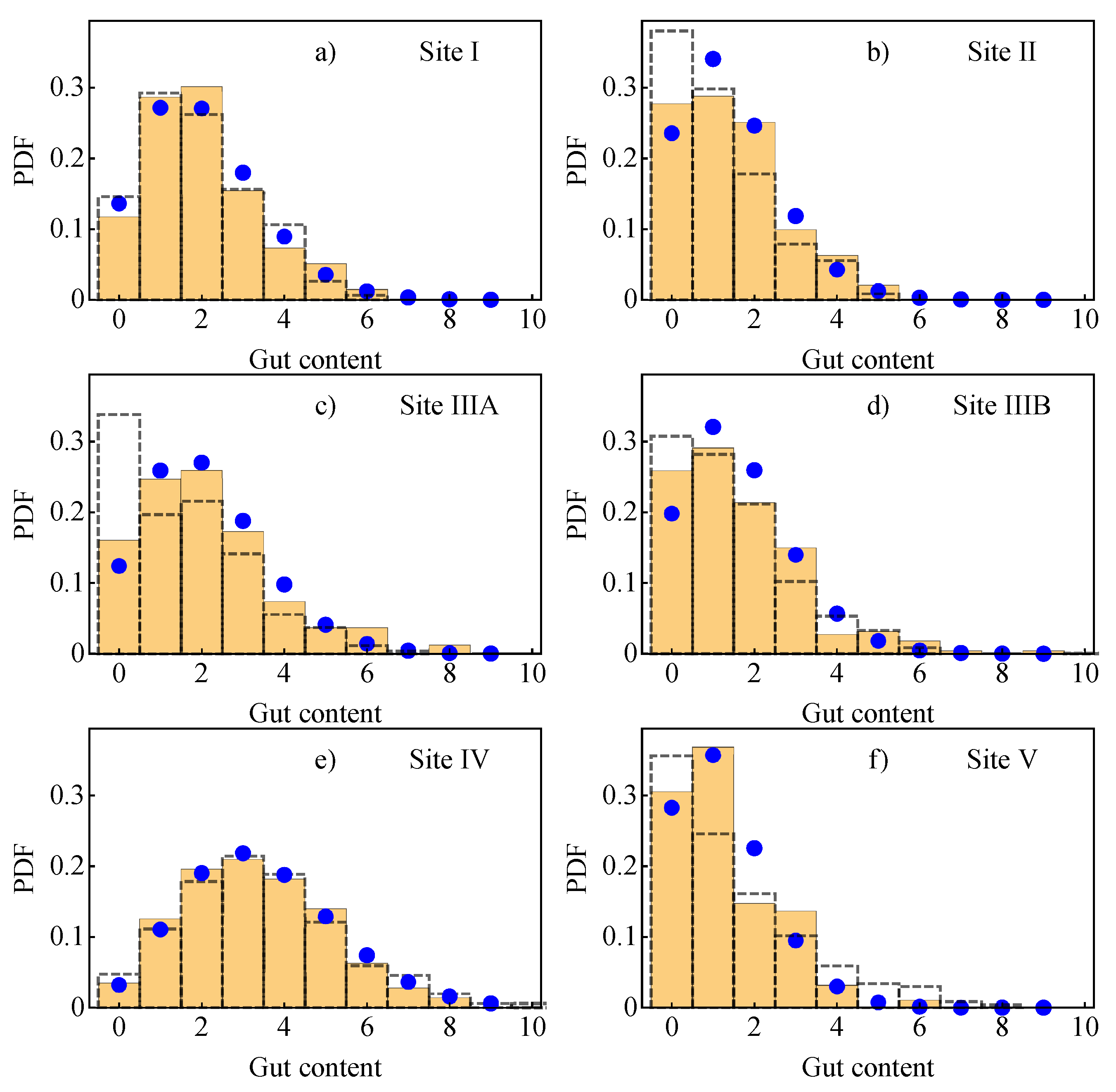
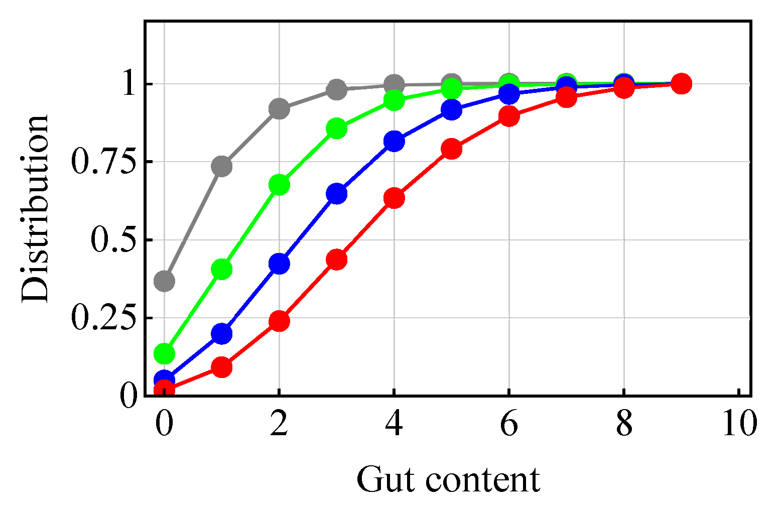
2.1.3. Probability Density of Gut Content

Encountered and captured prey contributes to the gut content of the predator, and will remain detectable until it is digested after some time (“gut clearance rate”), here denoted ${\tau }_d$. A simple model was proposed [18] for the gut content in form of a time series containing integers, $N=1,2,\dots ,N_m$ where N is the number of prey in the gut with $N_m$ being some maximum gut capacity. The maximum gut capacity has only little consequence for the data presented in the following, but the general results can be useful for other data. A relatively simple analysis [18] including a finite gut capacity gave the result

$$P_d\left(N\right|N_m)=\frac{exp(-\mu {\tau }_d)\mathrm{\Gamma }(2+N_m)}{(1+N_m)\mathrm{\Gamma }(1+N_m;\mu {\tau }_d)}\sum _{j=0}^{N_m}{\delta }_{j,N}\frac{{\left(\mu {\tau }_d\right)}^j}{j!}$$

(9)

for the normalized probability density in terms of the one-variable $\mathrm{\Gamma }\left(y\right)$-function and the two-variables incomplete $\mathrm{\Gamma }(y;z)$-function [46]. We introduced the Kronecker ${\delta }_{j,N}$ which is unity if $j=N$, and zero otherwise. We assume $N_m$ to be given. The result has then no free adjustable parameters since the product $\mu {\tau }_d$ consists of measurable quantities. In nature we often found guts to be nearly empty and in such cases the finite gut capacity is of no consequence for the probability density. We can then use a simpler expression

$$P_d\left(N\right)=\sum _{j=0}^{\infty }{\delta }_{j,N}\frac{{\left(\mu {\tau }_d\right)}^j}{j!}exp(-\mu {\tau }_d).$$

(10)

It is interesting to note that $\mu$ and ${\tau }_d$ appear in (9) as well as in (10), only as a product and not individually. From simple dimensional arguments [47] this could have been seen from the outset. We find this result to be important: if the distribution of gut content can be estimated and ${\tau }_d$ is known for the predator, we can find $\mu$ for the given organisms and conditions in the environment. This value for $\mu$ can then be compared to analytical results.

At first sight the arguments giving (9) and (10) seem to contain a flaw: it presumes $N_m$ to be a fixed deterministic number and thereby all prey to have the same size. In reality we can have many small or a few large samples of prey in a full gut. This question was discussed elsewhere [18] with an assumed probability density for prey sizes. The result indicated that if the number of prey in the gut is large, some will be small, some large, so the actual net gut content would be close to the one obtained by assigning all prey the same size. In addition we note that the distribution of captured prey lengths (nauplii) had a distribution that was narrow compared to the average value, as demonstrated later.

2.2. Field Data

Our observational data are based on samples collected at Lofoten, Norway in April–May 1995 [18,48]. During this campaign data were collected at 5 sites, labeled Station I, II, III, IV and V, all located in shallow waters, see Figure 6. The conditions were strongly influenced by tidally-induced turbulence and turbulence induced from long swells. At one of the sites (Station III) the turbulence conditions changed during the day so we have two data-sets there, Station IIIA and Station IIIB. In the beginning of May the sun rises around 04 and settles around 22 local time. Sample collection was restricted to the time interval 06–22 in order to eliminate effects of reduced feeding/ingestion rates during the dark part of the day. The varying light conditions during the day were similar for each site [40].

The methodology of the plankton sampling and analysis, i.e. the vertical sampling of the cod larvae and their naupliar prey and the analysis of the gut content of the cod larvae, was adopted from previous studies [21,22]. The vertical concentration profile of fish larvae was determined by a fish larvae pump with a capacity of approximately 0.5–0.7 m${}^3$s${}^{-1}$. A plankton net with 375 $\mathsf{\mu }$m mesh size was attached to the fish larvae pump. Samples were made at discrete depths from 5 m to 40 m. It was anticipated that the pump may cause some damage to the collected fish larvae. The damage is known to depend on the duration of the pumping times, in our case they varied from 15 s to 60 s. The quality of these data has therefore to be verified by another collection methods which do not have such a damaging effect. Fish larvae were also sampled by a vertically hauled plankton net. The opening of the net was 0.5 m${}^2$ with a 375 $\mathsf{\mu }$m mesh size. The net was hauled vertically from 50 m depth, or from approximately 2 m above the seabed when the water was shallower than 50 m. From the collected fish larvae those in the start-feeding phase (stage 7 larvae [21]) were selected and their lengths measured. Their gut content was inspected by counting the number of prey carcasses in the gut of fish larvae. The length distribution of cod larvae from a selected site is illustrated in Figure 7. Similar distributions were obtained from the other sites as well.

A measurement based on 299 cod larvae gave a distribution of the lengths a of the nauplii found in the guts, see Figure 8. The most probable nauplii length was found to be approximately 200 $\mathsf{\mu }$m. The spread in the sizes is noticeably smaller than the average.

Figure 9 shows the vertical distribution of predators (here Gadus morhua L.) at Sites I to V. Data were collected at times evenly distributed over the day, but the number of samples collected varied from site to site. We find indications of a systematic variation with depth only at Site V and even here it is not significant.

Figure 10 shows the vertical distribution of prey (here nauplii) at Sites I to V, sampled with a pump with plankton net mesh size 90 micrometers. Data were collected at times evenly distributed over the day, but the number of samples collected varied from site to site. We find no systematic variation of the density of nauplii with depth, and assume that the turbulent mixing is sufficient to smooth out gradients in the nauplii distribution for the present shallow waters. We note that the variability of measured nauplii concentration from one measurement to the other is the smallest for the site with smallest turbulence intensity. In the lack of any systematic depth variation of the nauplii distribution we assign each site as reference concentration the average over all depths for that site.

Figure 11 shows scatter diagrams for the sizes of cod larvae and their gut contents. The correlations are in general not sufficient to allow conclusions of substance. The scatter in larvae size is moderate due to the pre-selection, and a high correlation between the size of cod larvae and their gut content can not be supported by the present database. Mostly we find a reasonable result indicating that large fish-larvae are most efficient in capturing prey.

The largest number of nauplii found in a gut was 12, and this number was observed only once. A gut content of 10 and 11 was both seen 4 times, while 9 nauplii were observed frequently. In the following we use $N_m=9$ for all the fish larvae. Based on data obtained by the vertically hauled plankton net we estimated the distributions of the gut contents as shown in Figure 12. The net gives the least damage to the cod larvae, and the data for these are therefore analyzed separately. Filled circles in each of the Figure 12 give results derived by the analytical model (9) by adjusting the parameter $\mu {\tau }_d$ so that the average corresponds to the observed value of $\langle N\rangle$. The results were obtained for $N_m=9$ as mentioned. Taking $N_m=10$ gave modification that were noticeable only for Site IV, with results shown elsewhere [18]. In order to quantify the difference between the model results and the observations we note that for small $\mu {\tau }_d$, the model predicts $(\langle N^2\rangle -{\langle N\rangle }^2)/\langle N\rangle =1$. When taken as an average for all the datasets shown in Figure 12, the same quantity was found to be 1.18. We find this agreement to be sufficiently convincing to allow the model (9) to be used also more generally. For completeness we included with thin dashed lines in Figure 12 also the results found by using data collected via the fish larvae pump. Implicit in the derivation is the assumption that the gut content PDF’s are time stationary.

Comparing the data found by the vertically hauled ichthyoplankton net and fish larvae pump as shown in Figure 12 we note a systematic overpopulation of empty guts (best seen for Site IIIA) in the data obtained by use of the pump. We take this as evidence that the pump is damaging plankton by making a significant part of them regurgitate. Existing and future data obtained by pumps like these should be interpreted with this possibility in mind. Because of the uncertainty associated with the data collected by the pump, we use only results for the vertically hauled net for comparison with analytical results. The depth resolution of the distribution of cod larvae and the corresponding gut content is then lost. The depth distribution of the number of cod larvae as found by the pump remains useful. Also earlier investigations [21,22] used the pump profiles to get an estimate of the vertical distributions of the larvae, while the gut contents were examined from the more gentle sampling by vertical net hauls.

Since the typical gut evacuation rates in first-feeding cod larvae are of the order of 1 h, it cannot be expected that the ambient food concentration of the cod larvae is equal to the sampling depth. Cod larvae are able to move vertically considerable distances during 1 h, up to 20 m. In addition, stronger mixed-layer turbulence can move the larvae even more during this period of time. Referring to Figure 10 we note that the vertical prey (nauplii) distribution was on average fairly uniform.

For a given average value of the capture rate $\mu$ for a population, some cod larvae will have more, some less than the number needed for survival. To give a convenient estimate for the gut contents we take the cumulative distributions for the number of prey in the guts of fish larvae (9) as shown in Figure 13 for the parameter values $\mu {\tau }_d=1,2,3$ and 4. Taking for instance the case with $\mu {\tau }_d=2$ (green curve) we find that a fraction 0.85 of the cod larvae have 3 nauplii or less in their gut, while for $\mu {\tau }_d=4$ (red curve) this fraction is 0.45. When ${\tau }_d=1$ h the values for $\mu$ are also the number of nauplii captured per hour. By the Figure 12 we found $\mu {\tau }_d=1.99,1.45,2.09,1.62,3.34,$ and 1.26. Taking here for illustration ${\tau }_d=45$ min, we consequently have $\mu =2.65,1.93,2.79,2.16,4.45$ and 1.68 captured nauplii per hour on average. These numbers should be compared to 2–3 nauplii per hour needed by cod larvae for survival.

In Table 1 we present a summary of averaged data as they are used for the comparison with analytical results. The set of observations at a given site are considered as individual realizations belonging to an ensemble with the given macroscopic parameters. The average number $\langle N_H\rangle$ of nauplii in gut is obtained by the reduced database found by using the fine meshed net moved slowly from the sea-bottom to the surface. The cod larvae mean length is $\langle L_{\ell }\rangle$, the concentration of nauplii in the surroundings is given by $D_0$, and the mean length of nauplii is $\langle a\rangle$. The specific turbulent energy dissipation is $ϵ$, and the derived effective Kolmogorov length ${\eta }_0$ is determined for each site as discussed in the following Section 2.2.1. The Kolmogorov time scale is ${\tau }_K=\sqrt{\nu /ϵ}$.

Ambient temperatures ranged from $4.5^{\circ }$ to 5.5 ${}^{\circ }$C. The salinity ranged from 33.5 to 34, corresponding to a kinematic viscosity of the water $\nu =1.5$ mm${}^2$s${}^{-1}$ [49,50].

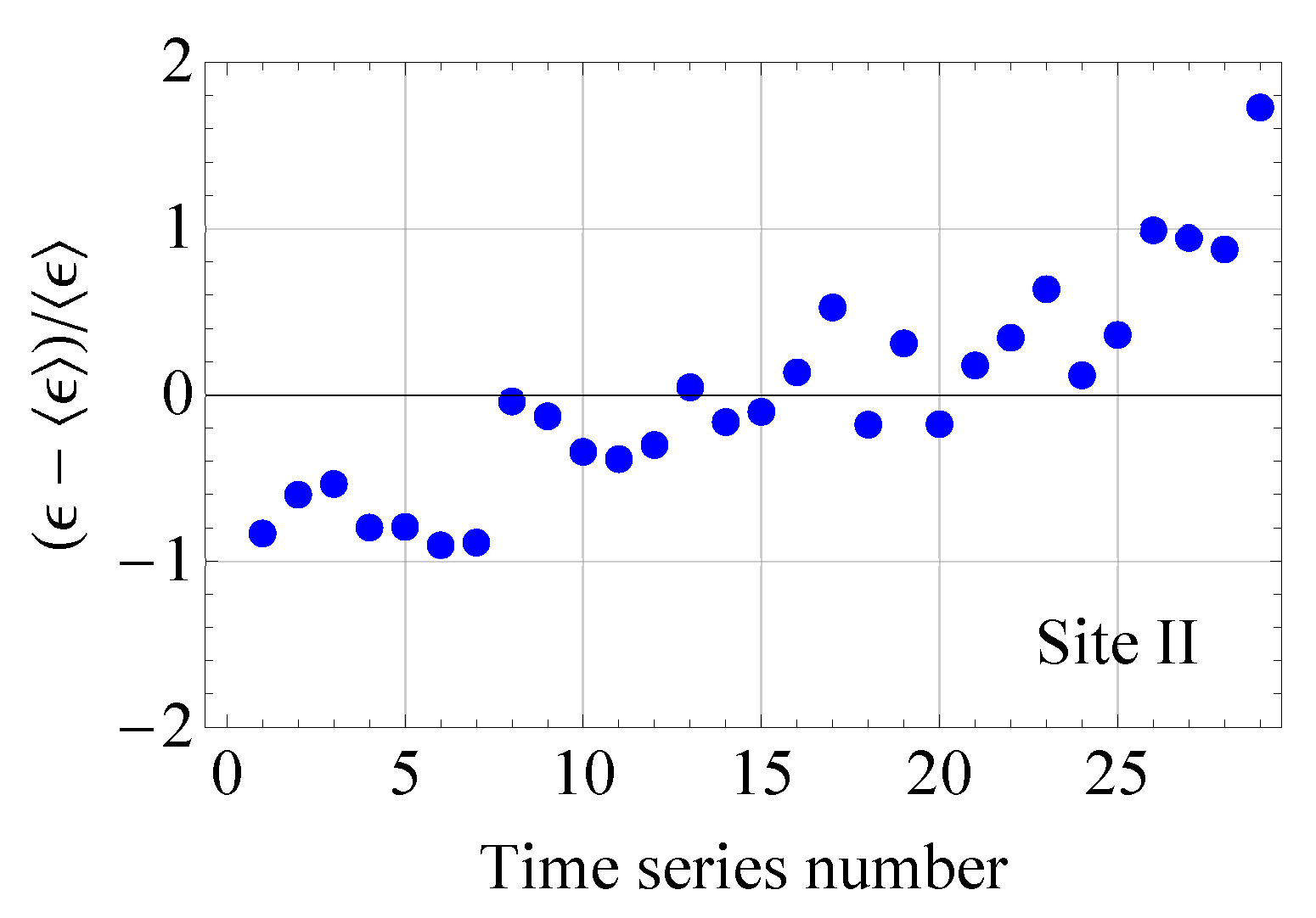
2.2.1. Estimates of the Average Specific Turbulent Energy Dissipation Rate

As we have seen, the turbulent energy dissipation rate $ϵ$ is an essential parameter for describing turbulence in the inertial as well as the viscous subranges. When only a one-point measurement is available, the almost universally adopted method for determining $ϵ$ relies on the Taylor hypothesis, or the frozen turbulence approximation [51,52,53,54,55,56,57]. It is there argued that a detected frequency spectrum can be “translated” to a wavenumber spectrum by $k\approx \omega /V$ where V is a constant average relative flow velocity between the rest frame of the fluid and the detector. In effect, it is assumed that the Doppler shift $kV$ dominates the rest frame frequency ${\omega }^{\prime }$, i.e., $\omega ={\omega }^{\prime }+kV\approx kV$. Local homogeneity and isotropy of the turbulence is implicitly assumed when applying Taylor’s hypothesis for interpreting turbulent power spectra. In case there is no average flow it will still be so that the small eddies in the inertial subrange are advected by the larges energy containing eddies [53] and the hypothesis can be applied also then, now with a suitably defined RMS fluid advection velocity. Details of the analysis and procedures used in the present work are reported elsewhere [55].

Fluctuating flow velocity components were detected by three different high resolution acoustic current meters (an Ocean ADV from NORTEK, a MINILAB and an UCM from SimTronix) were mounted on a submarine tower 6.5 m above the seabed [18,48]. All instruments were facing upwards in order to minimize possible effects of the construction on the observations. All data reported in the present work are obtained by the UCM, which measures the 3 velocity components of the fluctuating flow with a minimum resolvable wavelength of approximately 2 cm. In Figure 14 we show typical values for average horizontal velocities found to be in the range 5–10 cm s${}^{-1}$. Most of the kinetic energy in the fluid motion is associated with the largest non-universal eddy dynamics. Taylor’s hypothesis gives most accurate results for large velocities [52], but there seems to be no universally accepted reference velocity expressed in terms of the flow parameters.

Results for the experimentally obtained spectra for the three fluctuating fluid velocity components are shown in Figure 15. Due to the closeness of sea-bottom, the vertical component has a reduced intensity at small frequencies (corresponding to long wavelengths) but the three spectra are close for high frequencies (i.e., short wavelengths), where we argue that local isotropy and homogeneity has been reached for the small scales. The observation that a frequency spectrum with the Kolmogorov-Obukhov exponent at high frequencies, i.e., ${\omega }^{-5/3}$, is a good approximation can be taken as a support for the applicability of Taylor’s hypothesis. The swells could be identified directly in the raw data as large amplitude intermittent oscillatory “bursts”, and these contribute to the low frequency non-universal parts of the spectra.

Power spectra for the three components of velocity fluctuations were measured at each site. The variations in the local flow velocity were sampled with a frequency of 2 Hz, using time series of 20 min duration. The average turbulence energy dissipation rate $ϵ$ was determined by fitting experimentally obtained power spectra to the analytical Kolmogorov-Obukhov wave-number spectrum $C_{KO}{ϵ}^{2/3}{k}^{-5/3}$ that contains $ϵ$. The universal Kolmogorov constant is $C_{KO}\approx$ 0.5–1.5. As mentioned before, the comparison between the experimental frequency spectra and the theoretical wavenumber spectrum is made by reference to Taylor’s hypothesis [51,52,53,55,58]. The robustness of the analysis giving $ϵ$ is tested by using slightly different values of the exponent in the power-law, e.g., ${\omega }^{-2}$.

Since the experimentally obtained spectral index agrees with the analytical $-5/3$-law, we have the main uncertainty in the estimate of $ϵ$ to be in the use of Taylor’s hypothesis and the uncertainty of the translational velocity being used. The experimentally obtained values of $ϵ$ vary over the time series as can be seen in the relative variation $(ϵ-\langle ϵ\rangle )/\langle ϵ\rangle$ at Site II, see Figure 16, where $\langle ϵ\rangle$ is here the average value of $ϵ$ for the given site. The Figure 16 is representative for the other sites as well [18]. Also the results for the turbulent energy dissipation $ϵ$ are included in Table 1.

For conditions in the present study, the turbulence was dominated by tides and swells at the observation sites, and thus different from earlier studies [21] and [22] where wind-induced turbulence dominated.

2.2.2. Comparison of the Analytical Model for Capture Rates and the Field Data Results

We made a comparison between our theoretical model and data obtained by analyzing the field observations. We found that under statistically time stationary conditions the average value of the gut content gives an estimate of $\mu {\tau }_d$. Given an estimate for the digestion time ${\tau }_d$, which has to be found by other means, in a laboratory for instance, we can then determine $\mu$ for the conditions specifying the predator and its environment. Gut evacuation rates were reported in [59], for instance. These rates can depend on temperature as well as other conditions [40]. These conditions can be assumed to be the same at all sites for our data. With the given selection of cod larvae we can assume that all predators are characterized by approximately the same parameters, so the differences are to be found in the environment. We have these parameters determined by the turbulence conditions $ϵ$ and availability of prey $D_0$, both parameters measured, while the viscosity $\nu$ is determined by the temperature and salinity of the ambient water.

The comparison between the analysis and the present field data is shown in Figure 17. In previous studies of the dataset [18] it was noted that all predator sizes were below ${\eta }_0$ and thus in the viscous subrange, see also Table 1. The capture range $R_c$ can however be larger than the cod larvae and it is then possible that the overlap region between viscous and inertial subranges have to be included in a complete analysis. This has a price, however: even after normalizing the capture rate by $D_0{R}_c^3$ it is found that the complete analytical model depends explicitly on both $ϵ$ and $R_c$, see for instance (4). The viscous subrange taken alone is simpler in this respect. In Figure 17 we thus show a surface spanned by the variables $ϵ$ and $R_c$ both in physical units. The variation of the capture rate is given through a normalization as $\mu t_m/\left(D_0{R}_c^3\right)$. We assumed the minimum time needed for capture to be $t_m=3$ s as a representative value [13]. Because of the uncertainties associated with the gut-content data obtained by the pump, we used only data from the vertically hauled plankton net for Figure 17. For the digestion time we took ${\tau }_d=45$ min, although also longer times have been argued [59]. The analysis is trivially remedied to account for other values of ${\tau }_d$, see for instance [18]. For the capture range we took $R_c=2L_{\ell }$, see Table 1. This gives $R_c$ in the range of 8–9 mm to be measured from the “center of mass” for the cod larvae. For the highest turbulence level, at Site IIIA, this value places $R_c$ between the viscous and inertial subranges. This observation demonstrates the need for a model that encompasses both the inertial and the viscous subranges in describing the encounter and capture rates for predators and prey.

As an alternative presentation we show in Figure 18 a projection of the data-points on a plane that cuts the surface in Figure 17 at the position defined by the average of the 6 values of $R_c$’s used there. The cut is shown by the blue line in Figure 18. Since the scatter in $R_c$-values as shown in Table 1 is moderate, we believe this figure also gives a useful illustration. A comparison with the analysis given elsewhere [18] illustrates the importance of including the correction from the inertial subrange. If this contribution is ignored, the dependence on $R_c$ will as mentioned before only enter through the normalization of the vertical axis. In that case a 2 dimensional presentation as in Figure 18 will be adequate without the need of a projection. For $R_c$ in the viscous subrange, the optimum capture value is found at $t_m\sqrt{ϵ/\nu }\sim 1$ with $\mu \sim D_0{R}_c^3/t_m$. The optimum thus obtained should be compared to the value of 2–3 nauplii captured per hour generally assumed to be needed for survival of cod larvae at the given stage. The digestion time ${\tau }_d$ does not enter here.

The analysis and the present dataset supports, in particular, elements of a “dome shaped” capture probability [13] in the sense that we find a decreasing trend in the average capture probability for increasing large turbulence levels.

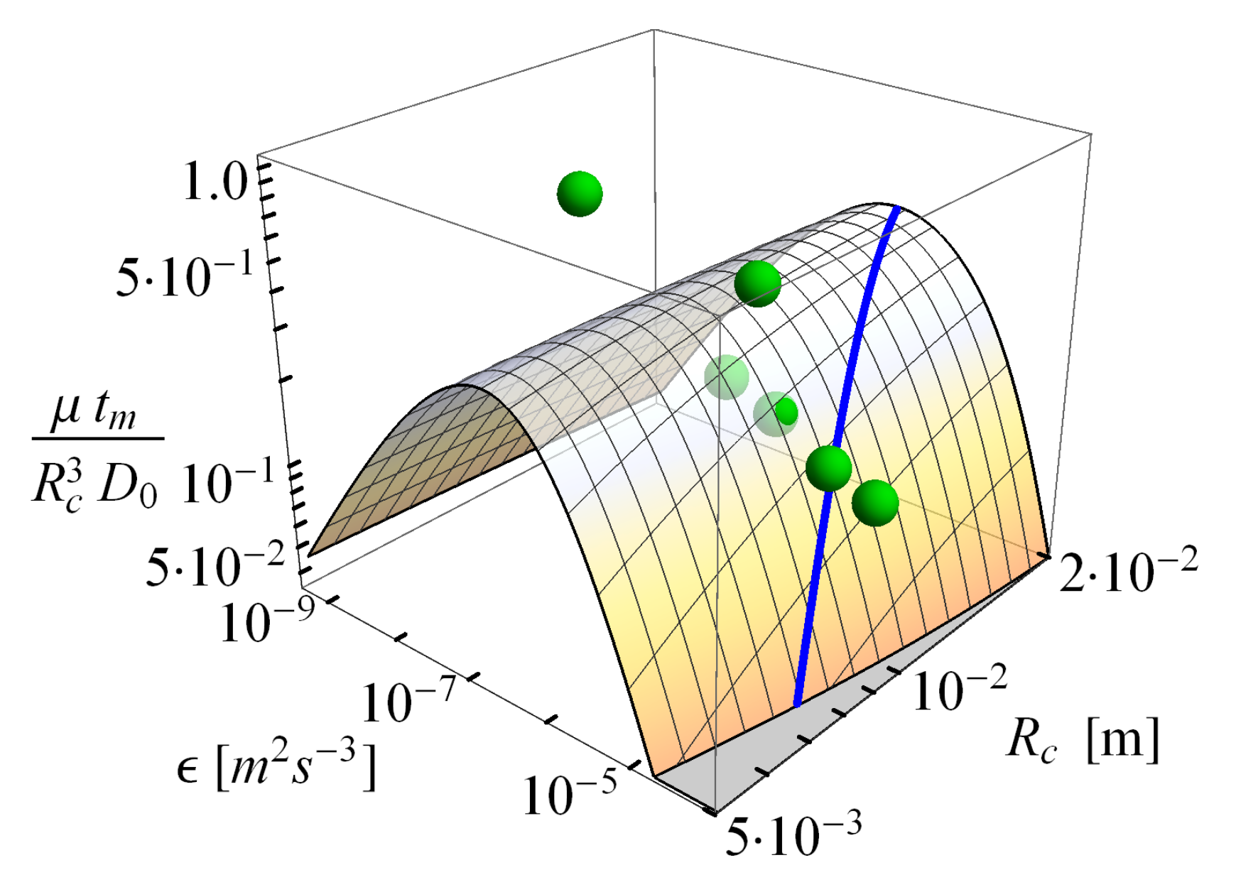
2.2.3. Consequences of Finite Sizes

As most other relates studies, also we described plankton as point-particles moving in the flow. A generalization of the study can be based on the Basset-Boussinesq-Oseen (BBO) equation derived for describing motions of finite size spherical particles in Stokes flows. A rigorous derivation [60] includes the effects of nonuniform velocity fields. The result is an analytical expression describing the motion of a spherical particle with given radius and mass, including the effects of gravitational acceleration. Most relevant aquatic organisms have mass density close to that of water. We therefore believe the finite size effects to be the most important, and will here briefly discuss some analytical models that can account for finite particle sizes [10,61]. These models represent a generalization of the Faxen corrections. The Stokes drag will be ignored here, although this effect can be included as well [61]. Our basic assumption is that a body with fixed shape responds to the moving flow by averaging the unperturbed space-time varying fluid velocity over its volume. This assumption seems reasonable and has shown promise when analyzing finite size particles moving in inhomogeneous pipe flows [62]. The averaging is most easily carried out in a spectral representation by a filtering, where the filter characteristics are determined by the particles (here plankton) in question [10,61]. For isotropic finite size particles we write an effective velocity as $\upsilon (\mathbf{r},t)={\int }_{-\infty }^{\infty }\mathcal{F}\left(k\right)\mathbf{u}(\mathbf{k},t)exp(i\mathbf{k}·\mathbf{r})d\mathbf{k}$ where $\mathcal{F}\left(k\right)$ is a filter function. The only basic requirements are $\mathcal{F}(k\to 0)\to 1$ and $\mathcal{F}(k\to \infty )\to 0$. For spherical particles, the filtering is simple. Anisotropic particles have interesting flow properties [10,61], but these are of limited relevance here and will not be discussed.

To illustrate the consequences of finite particle sizes for the modeling we consider here spherical encounter surfaces with range R in the inertial subrange of turbulence, and will later discuss the problems in generalizing these results to the viscous subrange. Apart form a numerical constant, the relation (2) can be obtained by the longitudinal second order structure function

$$U^2\left(r\right)\equiv 〈{\left(u_{\Vert }(\xi ,t)-u_{\Vert }(\xi +r,t)\right)}^2〉,$$

written in one spatial dimension for simplicity, with more details given elsewhere [8]. We have the reference predator to be at position $\xi$ and prey to be at $\xi +r$. For homogeneous isotropic turbulence conditions, we have $U\left(r\right)$ to be independent of $\xi$ and only the separation r enters. For the inertial subrange we know that $U^2\left(r\right)\sim {\left(ϵr\right)}^{2/3}$. Taking the flux to a reference point particle (the predator in our case) through a spherical encounter surface with surface area $\pi R^2$ we can use the encounter estimate $J\sim D_{0}U\left(R\right)R^2$, again apart from a numerical constant which is best determined empirically by experiments. Use of the previous expression for $U\left(R\right)$ in the inertial subrange gives $J\sim D_0{ϵ}^{1/3}{R}^{7/3}$ which is consistent with the result (2). With these results in mind we consider a finite size particle and apply the appropriate filtering to get a more general second order structure function in the form

$$U^2\left(r\right)=〈{\left({\int }_{-\infty }^{\infty }\left(\mathcal{F}\left(k\right)u_{\Vert }(k,t)-u_{\Vert }(k,t)exp\left(ikr\right)\right)exp\left(ik\xi \right)dk\right)}^2〉,$$

(11)

where we still consider prey as point particles, so that velocity is not filtered. After some manipulations reported elsewhere [63,64] an expression is obtained in the form

$$U^2\left(r\right)={\int }_{-\infty }^{\infty }\mathcal{E}\left(k\right)\left(1+{\left|\mathcal{F}\left(k\right)\right|}^2-2\mathcal{F}\left(k\right)exp\left(-\frac{1}{2}{k}^2{r}^2\right)\right)dk,$$

(12)

where the power spectrum for the fluctuating velocity is $\mathcal{E}\left(k\right)\equiv \langle u_{\Vert }(k,t)u_{\Vert }(-k,t)\rangle =\langle |u_{\Vert }\left(k\right){|}^2\rangle$ for time stationary conditions. At one place we approximated the average of a product by the product of two averages to have $\mathcal{E}\left(k\right)$ appearing explicitly and used also $\langle exp\left(ikr\right)\rangle =exp\left(-k^2{r}^2/2\right)$ as for Gaussian processes. If we ignore intermittency corrections and take the Kolmogorov-Obukhov spectrum as $\mathcal{E}\left(k\right)\sim {ϵ}^{2/3}{k}^{-5/3}$ in (12), together with the limiting form $\mathcal{F}\left(k\right)\approx 1$ for point particles we recover $J\sim D_{0}U\left(R\right)R^2\sim D_0{ϵ}^{1/3}{R}^{7/3}$ analytically for $r=R$. The other limiting case where $\mathcal{F}\left(k\right)\approx 0$ corresponds to a predator at rest, i.e., a “tethered” predator, where $J\sim D_0{R}^2\sqrt{\langle u^2\rangle }\gg D_0{ϵ}^{1/3}{R}^{7/3}$ where $\langle u^2\rangle ={\int }_{-\infty }^{\infty }\mathcal{E}\left(k\right)dk$. This latter result has experimental support [8]. For the case where R is much larger than the reference particle, we have $exp\left(-k^2{R}^2/2\right)\approx 0$ while $\mathcal{F}\left(k\right)\approx 1$; in this limit the finite size of the predator is immaterial, as also expected intuitively. The intermediate case with some general form for the filter $\mathcal{F}\left(k\right)$ is more problematic and will depend on the shape modeled by $\mathcal{F}\left(k\right)$. For illustration we assume $\mathcal{F}\left(k\right)=exp(-k^2{S}^2)$ where S represents a characteristic size of the predator, $S<R$. Using again the Kolmogorov-Obukhov spectrum for $\mathcal{E}\left(k\right)$ we have

$$J\sim D_0{ϵ}^{1/3}{R}^2\sqrt{{(R^2+2S^2)}^{1/3}-S^{2/3}{2}^{-1/3}}<D_0{ϵ}^{1/3}{R}^{7/3}\mathrm{for}R>S.$$

(13)

Within this model we find that the encounter rate is reduced compared to the results for plankton moving like point particles, i.e., $J_{e,I}$ in (2). Taking $R\approx 2S$ as used in the foregoing analysis we have a reduction of approximately 10% as compared to $J_{e,I}$.

We have thus found a viable model for including finite size effects where some limiting cases can be tested, provided we restrict the analysis to the inertial subrange of turbulence. This subrange is, however, restricted to wavenumbers smaller than the Kolmogorov wavenumber. The problem in generalizing the model to the viscous subrange is due to the lack of a universal spectral model for this limit. The analysis of Heisenberg [65] predicted a $\mathcal{E}\left(k\right)\sim k^{-7}$ power law spectral variation for large k, but this result makes ${\int }_{-\infty }^{\infty }{k}^{2p}\mathcal{E}\left(k\right)dk$ diverge for sufficiently large p-values, and the same can be argued for any power-law $\mathcal{E}\left(k\right)\sim k^{-m}$. This divergence is considered to be unphysical [66] and for the time being we have no generally accepted spectrum for the viscous subrange. For the second order structure function we have no similar problems. Assuming that the trends found for the inertial subrange apply to the viscous subrange as well, we argue that finite size effects give rise to a reduction factor of 10% also here. The uncertainty introduced by this is comparable to or even less than other uncertainties in the problem. Finite size effects are considered to have minor importance for our analysis but might be relevant other studies.

3. Discussion

We took the digestion time ${\tau }_d$ to be constant. In principle it is possible for ${\tau }_d$ to depend on the gut content. Our data give no support for such models [59]. Should that be the case, we would observe a systematic overpopulation for small or for large gut contents as compared to our model. It is possible that such a relation can be found by studies of populations where full guts are more frequent than in our database.

In the presentations in Figure 17 we ignored the prey escape reactions by setting $P_{es}=1$ in (8). Since $P_{es}$ accounts for the fraction of the prey density $D_0$ that escapes capture, we can change the normalization on the vertical axis in Figure 17 to $\mu t_m/\left(D_0{P}_{es}{R}_c^3\right)$ and the analytical part of the figure will then apply more generally. The points for the observations (green spheres) will then have to be moved upwards for $P_{es}<1$.

The assumed value for the minimum time needed for capture, $t_m=3$ s, may appear to be large, but it represents an average of the minimum time required for capture and the time needed for capture with large probability [29]. With this in mind we find the value $t_m=3$ s to be reasonable. The most sensitive parameter in the analytical model is $R_c$ by entering to the power 3.

The largest deviation between the data and the analytical model is found for the smallest turbulence level at Site IV at the head of the Austnesfjord. We have no verifiable explanation for this deviation, but note that self-induced motions will have the strongest effects for small turbulence levels, see (6) and Figure 5. The present analysis assumes that the cod larvae are ambush predators and ignores self-induced motions entirely. This assumption need not be strictly fulfilled, and we see this as a possible explanation for the noted disagreement. Self-induced motions will enhance the encounter rate. Using (6) we find, however, that excessively large values of $V_c$ need to be introduced in order to make the analytical result close to observations. Based on our data, we find however one conclusion to be inescapable: turbulence matters!

Possible sources for errors in the data analysis, be it systematic or random, have been discussed elsewhere [18] and the comments there apply equally well to the present analysis. We believe that the most significant uncertainty is associated with the estimates of $ϵ$, see also Figure 16.

The conditions characterizing the present set of field data differs from other studies by the source of the turbulence generation. With the exception of Site IV placed at the head of the Austnesfjord, we find the dominant energy sources to be swells and tidal motions, in contrast to wind generated turbulence [67]. Results for this latter case are usually presented in terms of an ocean surface wind velocity W and a depth Z, referring to a an empirical relation

$$ϵ=5.8\times {10}^{-9}\frac{W^3}{Z},$$

(14)

expressing $ϵ$ in units of ${\mathrm{m}}^2{\mathrm{s}}^{-3}$, W in $\mathrm{m}{\mathrm{s}}^{-1}$ and Z in m. For such conditions a predator can change its vertical position to obtain optimum conditions [68,69]. For our dataset the model (14) is not applicable. Wind generated turbulence was the dominant source of turbulence in other studies [21,22].

The target species of the present study, i.e., first-feeding cod larvae preying on copepod nauplii, and the biological sampling methods, as outlined above, were the same as those used in the earlier field studies [21,22]. The study locations and the methods representing ambient turbulence for the organisms, however, differed substantially. While the studies [21,22] were conducted above the deep-water areas (bottom depths 80–150 m) of the Lofoten nursery grounds, where pelagic-layer turbulence is mainly produced by wind mixing, the present study was conducted in the shallow-water regions (bottom depths 17–30 m) where the turbulence is largely produced by near bottom tidal current shears and also by swells. The two earlier studies [21,22] were conducted without measuring mixed-layer turbulence, since the authors at that time did not have access to free-falling airfoil probes [70] to profile turbulence through the upper layer. Therefore, an empirical relationship established between winds and turbulent energy dissipation rates [23] was applied to estimate the ambient turbulence of the organisms studied. The present study, on the other hand, was motivated by how tidal-induced turbulence, generated from the bottom, might differ from wind-induced turbulence of the mixed layer, generated from the surface of the ocean. The turbulence measurements used here, were made with acoustic current meters on top of a 6.5 m high tower deployed on the seabed. Differently from profiling airfoil probes, this allowed for generating time series of turbulence measurements. On the other hand, measurements were here limited to one vertical position.

As outlined before, the biological sampling technique of measuring the stomach fullness of a fish larvae predator, here quantified as the number of nauplii in the gut of the predator, reflects the integrated encounters between predator and prey over a time period of about 1–2 h prior to sampling. During this time span the predator can migrate and/or become transported vertically through the mixed-layer. Moreover, the predators and the prey will typically become horizontally advected by the currents at a distance of 0.5–2 km [71] over the same period of time. This justifies application of vertically averaged prey concentrations when comparing the number of prey in the gut of the predator. However, the two other major factors influencing predator-prey encounter rates, namely the turbulence and light conditions can both change systematically through the pelagic layer. Firstly, the turbulent energy dissipation rate generated from surface wind mixing is not vertically homogeneous through the upper part of the mixing layer as suggested by [23] but decreases by some empirical function [13] as for example in (14). Recent empirical studies based on the measurements from state-of-the-art turbulence profiler show that the turbulent energy dissipation rate changes with depth as $Z^{-1.15}$ over the mixing layer [72]. Secondly, there are indications of a certain variation in encounter rate with light intensity [22]. Since this intensity changes with depth as $e^{-\kappa Z}$, where $\kappa \sim 0.14$ m${}^{-1}$ for coastal waters [16], it is also expected that the vertical position of the predator will affect the prey encounter rate.

In summary, of the three factors influencing encounter rates for larval predators of the wind-mixed layer, i.e., prey concentration, light intensity and turbulence, the two latter factors have the most substantial (and systematic) decrease with depth. This implies that the exact vertical position within the mixed layer will have large impacts on the encounter rates experienced by the predator in a wind mixed layer.

From field observations of spatial distributions of first-feeding cod larvae we know that their vertical distributions vary considerably with light conditions and with the wind mixing [73,74]. Generally, first-feeding cod larvae are found at highest concentrations between 10 and 30 m depth, but there are large short-time variations over a wider vertical range, typically from 5 to 40 m depth [73]. During stronger wind mixing, larvae are dispersed vertically deeper down to even 50 m depth by vertical mixing/and or active migration [73]. This implies that the cod larvae by a change in vertical position may be able to adjust their turbulence-induced encounter rates to the optimum [13] and thereby avoid turbulence levels exceeding those for optimum encounter-capture rates. Over the vertical range observed for cod larvae (i.e., surface layer to 50 m depth) the wind-generated turbulent energy dissipation rate changes by two orders of magnitude [72]. The previous field experiments [21,22] covered wind-induced turbulence for wind speeds up to 11 m s${}^{-1}$. Most of the observations summarized there did not reach values of encounter rates for the larvae exceeding the optimal local maximum illustrated in, for instance, Figure 18. One single observation site in the former studies [22] was located in the same shallow-water and tidal-energetic region as for the present data. The Greenberg relation for turbulent energy dissipation rates [75] applied for those conditions indicated a turbulent energy dissipation rate $ϵ$ of the order of 10${}^{-6}$ m${}^2$s${}^{-3}$. The observed larval encounter rate for this situation was higher than for the highest wind-induced turbulent conditions (11 m s${}^{-1}$). The fish larvae were not exposed to turbulence levels exceeding the optimum of the “dome shaped” capture rate. Differently, in the present study of shallow-water depths of 17 to 30 m, the turbulent energy dissipation rates reached levels up to ${10}^{-4}$ m${}^2$s${}^{-3}$. With no possibility for the larvae to escape to greater depth, they became exposed to turbulence levels exceeding the optimum for encounters followed by capture.

4. Conclusions

The available data demonstrate the importance of the viscous subrange for describing the effects of turbulence on feeding conditions for plankton, but show also that a model is needed to account for the transition between viscous and inertial subranges of fully developed turbulence. Some of our data sampled in a shallow-water environment with high turbulence, demonstrate the reduction of capture probabilities caused by strong turbulent motions. Some cases are near the optimum level of the “dome shaped” capture rate. Only one case, from Site IV, falls in the range where turbulence has a purely advantageous effect. This site is located deep in a fjord with a lower level of turbulence. Within our database, the most advantageous site for the cod larvae is thus clearly in the Austnesfjord. Future studies of this problem should bear in mind that the relevant turbulence range is determined also by the contact range $R_c$ of the predator, so a given turbulence level can appear strong for some organisms, and weak for others.

The ideas advanced in the present study referred explicitly to aquatic organisms in a turbulent environment. Elements of the models may, however, have wider applicability. In discussions with one of the authors (HLP), Prof. Jukka Heikkinen draws attention to a different problem concerning burning of charcoal dust. This process is relevant, for instance, for disposing of charcoal in filters. The burning is accelerated by dispersing the charcoal dust in a very hot air (i.e., flames). In this case we can associate the charcoal particles (until they burn out) with the predators, while their prey is the Oxygen in the surrounding. The flames constitute the turbulent environment giving the enhanced mixing. In this case we can also assume the turbulence conditions to be well described by the inertial range of the Kolmogorov-Obukhov law and also include the universal dissipation range. We anticipate that the analysis of the present study can be generalized to account also for elements in the problem outlined here being aware, though, that very different effects are also at play there, such as radiative and thermal effects, and the fact the dust particles may adhere to each other.

References

1. Houde, E.D. Fish early life dynamics and recruitment variability. Am. Fish. Soc. Symp. 1987, 2, 17–29. [Google Scholar]
2. Houde, E.D. Subtleties and episodes in the early life of fishes. J. Fish Biol. 1989, 35, 29–38. [Google Scholar] [CrossRef]
3. Hinrichsen, H.H.; Möllmann, C.; Voss, R.; Köster, F.W.; Kornilovs, G. Biophysical modeling of larval Baltic cod (Gadus morhua) growth and survival. Can. J. Fish. Aquat. Sci. 2002, 59, 1858–1873. [Google Scholar] [CrossRef] [Green Version]
4. Lough, R.G.; Buckley, L.J.; Werner, F.E.; Quinlan, J.A.; Pehrson Edwards, K. A general biophysical model of larval cod (Gadus morhua) growth applied to populations on Georges Bank. Fish. Oceanogr. 2005, 14, 241–262. [Google Scholar] [CrossRef]
5. Rothschild, B.J.; Osborn, T.R. Small-scale turbulence and plankton contact rates. J. Plankton Res. 1988, 10, 465–474. [Google Scholar] [CrossRef]
6. Osborn, T. The role of turbulent diffusion for copepods with feeding currents. J. Plankton Res. 1996, 18, 185–195. [Google Scholar] [CrossRef] [Green Version]
7. Hill, P.S.; Nowell, A.R.M.; Jumars, P.A. Encounter rate by turbulent shear of particles similar in diameter to the Kolmogorov scale. J. Mar. Res. 1992, 50, 643–668. [Google Scholar] [CrossRef] [Green Version]
8. Mann, J.; Ott, S.; Pécseli, H.L.; Trulsen, J. Turbulent particle flux to a perfectly absorbing surface. J. Fluid Mech. 2005, 534, 1–21. [Google Scholar] [CrossRef]
9. Boffetta, G.; Pécseli, H.L.; Trulsen, J. Numerical studies of turbulent particle fluxes into perfectly absorbing spherical surfaces. J. Turbul. 2006, 7, N22. [Google Scholar] [CrossRef]
10. Pécseli, H.L.; Trulsen, J. Turbulent particle fluxes to perfectly absorbing surfaces: A numerical study. J. Turbul. 2007, 8, N42. [Google Scholar] [CrossRef]
11. Lewis, D.M.; Pedley, T.J. Planktonic contact rates in homogeneous isotropic turbulence: Theoretical predictions and kinematic simulations. J. Theor. Biol. 2000, 205, 377–408. [Google Scholar] [CrossRef] [PubMed]
12. Pécseli, H.L.; Trulsen, J.; Fiksen, Ø. Predator-prey encounter rates in turbulent water: Analytical models and numerical tests. Prog. Oceanogr. 2010, 85, 171–179. [Google Scholar] [CrossRef]
13. MacKenzie, B.R.; Miller, T.J.; Cyr, S.; Leggett, W.C. Evidence for a dome-shaped relationship between turbulence and larval fish ingestion rates. Limnol. Oceanogr. 1994, 39, 1790–1799. [Google Scholar] [CrossRef] [Green Version]
14. Jenkinson, I.R. A review of two recent predation-rate models: The dome-shaped relationship between feeding rate and shear rate appears universal. ICES J. Mar. Sci. 1995, 52, 605. [Google Scholar] [CrossRef]
15. MacKenzie, B.R.; Kiørboe, T. Larval fish feeding and turbulence: A case for the downside. Limnol. Oceanogr. 2000, 45, 1–10. [Google Scholar] [CrossRef]
16. Fiksen, Ø.; Utne, A.; Aksnes, D.; Eiane, K.; Helvik, J.; Sundby, S. Modelling the influence of light, turbulence and ontogeny on ingestion rates in larval cod and herring. Fisheries Oceanog. 1998, 7, 355–363. [Google Scholar] [CrossRef] [Green Version]
17. Vollset, K.; Folkvord, A.; Browman, H. Foraging behaviour of larval cod (Gadus morhua) at low light intensities. Mar. Biol. 2011, 158, 1125–1133. [Google Scholar] [CrossRef] [Green Version]
18. Pécseli, H.L.; Trulsen, J.K.; Stiansen, J.E.; Sundby, S.; Fossum, P. Feeding of plankton in turbulent oceans and lakes. Limnol. Oceanogr. 2019, 64, 1034–1046. [Google Scholar] [CrossRef]
19. Solberg, T.; Tilseth, S. Growth, energy consumption and prey density requirements in first feeding larvae of cod (Gadus morhua L.). In Proceedings of the Propagation of Cod Gadus morhua L., Arendal, Noway, 14–17 June 1983. [Google Scholar]
20. Sundby, S. Turbulence and ichthyoplankton: Influence on vertical distributions and encounter rates. Sci. Mar. 1997, 61, 159–176. [Google Scholar]
21. Sundby, S.; Fossum, P. Feeding conditions of arcto-Norwegian cod larvae compared with the Rothschild-Osborn theory on small-scale turbulence and plankton contact rates. J. Plankton Res. 1990, 12, 1153–1162. [Google Scholar] [CrossRef]
22. Sundby, S.; Ellertsen, B.; Fossum, P. Encounter rates between first-feeding cod larvae and their prey during moderate to strong turbulent mixing. ICES Mar. Sci. Symp. 1994, 393–405. [Google Scholar]
23. Oakey, N.S.; Elliott, J.A. Dissipation within the surface mixed layer. J. Phys. Oceanogr. 1982, 12, 171–185. [Google Scholar] [CrossRef]
24. Biferale, L.; Boffetta, G.; Celani, A.; Devenish, B.; Lanotte, A.; Toschi, F. Multifractal statistics of Lagrangian velocity and acceleration in turbulence. Phys. Rev. Lett. 2004, 93, 064502. [Google Scholar] [CrossRef] [PubMed] [Green Version]
25. Biferale, L.; Boffetta, G.; Celani, A.; Lanotte, A.; Toschi, F. Particle trapping in three-dimensional fully developed turbulence. Phys. Fluids 2005, 17, 021701. [Google Scholar] [CrossRef] [Green Version]
26. Tennekes, H.; Lumley, J.L. A First Course in Turbulence; The MIT Press: Cambridge, MA, USA, 1972. [Google Scholar]
27. Sreenivasan, K.R. On the universality of the Kolmogorov constant. Phys. Fluids 1995, 7. [Google Scholar] [CrossRef] [Green Version]
28. Davidson, P.A. Turbulence. An Introduction for Scientists and Engineers; Oxford University Press: Oxford, UK, 2004. [Google Scholar]
29. Pécseli, H.L.; Trulsen, J.; Fiksen, Ø. Predator-prey encounter and capture rates for plankton in turbulent environments. Prog. Oceanogr. 2012, 101, 14–32. [Google Scholar] [CrossRef]
30. Kiørboe, T. A Mechanistic Approach to Plankton Ecology; Princeton Univ. Press: Princeton, NJ, USA, 2008. [Google Scholar]
31. Pigolotti, S.; Jensen, M.H.; Vulpiani, A. Absorbing processes in Richardson diffusion: Analytical results. Phys. Fluids 2006, 18, 048104. [Google Scholar] [CrossRef]
32. Lewis, D.M.; Pedley, T.J. The influence of turbulence on plankton predation strategies. J. Theor. Biol. 2001, 210, 347–365. [Google Scholar] [CrossRef]
33. Lewis, D.M.; Bala, S.I. Plankton predation rates in turbulence: A study of the limitations imposed on a predator with a non-spherical field of sensory perception. J. Theor. Biol. 2006, 242, 44–61. [Google Scholar] [CrossRef]
34. Mann, J.; Ott, S.; Pécseli, H.L.; Trulsen, J. Laboratory studies of predator-prey encounters in turbulent environments: Effects of changes in orientation and field of view. J. Plankton Res. 2006, 28, 509–522. [Google Scholar] [CrossRef] [Green Version]
35. MacKenzie, B.R.; Kiørboe, T. Encounter rates and swimming behaviour of pause-travel and cruise larval fish predators in calm and turbulent laboratory environments. Limnol. Oceonogr. 1995, 40, 1278–1289. [Google Scholar] [CrossRef]
36. Reigada, R.; Hillary, R.M.; Bees, M.A.; Sancho, J.M.; Sagués, F. Plankton blooms induced by turbulent flows. Proc. R. Soc. Lond. Ser. B Biol. Sci. 2003, 270, 875–880. [Google Scholar] [CrossRef] [PubMed] [Green Version]
37. Durham, W.M.; Climent, E.; Barry, M.; De Lillo, F.; Boffetta, G.; Cencini, M.; Stocker, R. Turbulence drives microscale patches of motile phytoplankton. Nat. Comm. 2013, 4, 2148. [Google Scholar] [CrossRef] [Green Version]
38. Breier, R.E.; Lalescu, C.C.; Waas, D.; Wilczek, M.; Mazza, M.G. Emergence of phytoplankton patchiness at small scales in mild turbulence. Proc. Natl. Acad. Sci. USA 2018, 115, 12112–12117. [Google Scholar] [CrossRef] [PubMed] [Green Version]
39. Pécseli, H.L.; Trulsen, J.K.; Fiksen, Ø. Predator-prey encounter and capture rates in turbulent environments. Limnol. Oceanog. Fluids Environ. 2014, 4, 85–105. [Google Scholar] [CrossRef] [Green Version]
40. Dam, H.G.; Peterson, W.T. The effect of temperature on the gut clearance rate constant of planktonic copepods. J. Exp. Mar. Biol. Ecol. 1988, 123, 1–14. [Google Scholar] [CrossRef]
41. Marrasé, C.; Costello, J.H.; Granata, T.; Strickler, J.R. Grazing in a turbulent environment: Energy dissipation, encounter rates, and efficacy of feeding currents in Centropages hamatus. Proc. Nat. Acad. Sci. USA 1990, 87, 1653–1657. [Google Scholar] [CrossRef] [PubMed] [Green Version]
42. Saiz, E.; Kiørboe, T. Predatory and suspension-feeding of the copepod Acartia-tonsa in turbulent environments. Mar. Ecol. Prog. Ser. 1995, 122, 147–158. [Google Scholar] [CrossRef]
43. Kiørboe, T.; Saiz, E. Planktivorous feeding in calm and turbulent environments, with emphasis on copepods. Mar. Ecol. Prog. Ser. 1995, 122, 135–145. [Google Scholar] [CrossRef] [Green Version]
44. Pécseli, H.L.; Trulsen, J.K. Plankton’s perception of signals in a turbulent environment. Adv. Phys. X 2016, 1, 20–34. [Google Scholar] [CrossRef]
45. Kiørboe, T.; Visser, A.W. Predator and prey perception in copepods due to hydromechanical signals. Marine Ecol. Prog. Ser. 1999, 179, 81–95. [Google Scholar] [CrossRef] [Green Version]
46. Abramowitz, M.; Stegun, I.A. Handbook of Mathematical Functions with Formulas, Graphs, and Mathematical Tables; Dover: New York, NY, USA, 1972. [Google Scholar]
47. Buckingham, E. On physically similar systems; illustrations of the use of dimensional equations. Phys. Rev. 1914, 4, 345–376. [Google Scholar] [CrossRef]
48. Gytre, T.; Nilsen, J.E.O.; Stiansen, J.E.; Sundby, S. Resolving small scale turbulence with acoustic Doppler and acoustic travel time difference current meters from an underwater tower. In Proceedings of the OCEANS 96 MTS/IEEE Conference Proceedings, The Coastal Ocean—Prospects for the 21st Century, Fort Lauderdale, FL, USA, 23–26 September 1996; pp. 442–450. [Google Scholar]
49. Sharqawy, M.H.; Lienhard, J.H.; Zubair, S.M. Thermophysical properties of seawater: A review of existing correlations and data. Desalin. Water Treat. 2010, 16, 354–380. [Google Scholar] [CrossRef]
50. Sharqawy, M.H.; Lienhard, J.H.; Zubair, S.M. Erratum to Thermophysical properties of seawater: A review of existing correlations and data [Desalination and Water Treatment, Vol. 16 (2010) 354-380]. Desalin. Water Treat. 2012, 44, 361. [Google Scholar] [CrossRef] [Green Version]
51. Wandel, C.F.; Kofoed-Hansen, O. On the Eulerian-Lagrangian transformation in the statistical theory of turbulence. J. Geophys. Res. 1962, 67, 3089–3093. [Google Scholar] [CrossRef]
52. Shkarofsky, I.P. Turbulence in Fluids and Plasmas; Chapter “Analytic Forms for Decaying Space/Time Turbulence Functions”; Polytechnic Press: Brooklyn, NY, USA, 1969; pp. 289–301. [Google Scholar]
53. Tennekes, H. Eulerian and Lagrangian time microscales in isotropic turbulence. J. Fluid Mech. 1975, 67, 561–567. [Google Scholar] [CrossRef]
54. Wyngaard, J.C.; Clifford, S.F. Taylor’s hypothesis and highfrequency turbulence spectra. J. Atmos. Sci. 1977, 34, 922–929. [Google Scholar] [CrossRef] [Green Version]
55. Stiansen, J.E.; Sundby, S. Improved methods for generating and estimating turbulence in tanks suitable for fish larvae experiments. Sci. Mar. 2001, 65, 151–167. [Google Scholar] [CrossRef] [Green Version]
56. Trujillo, J.J.; Trabucchi, D.; Bischoff, O.; Hofsäß, M.; Mann, J.; Mikkelsen, T.; Rettenmeier, A.; Schlipf, D.; Kühn, M. Testing of frozen turbulence hypothesis for wind turbine applications with a Staring Lidar. Geophys. Res. Abstr. 2010, 12, 5410. [Google Scholar]
57. Geng, C.; He, G.; Wang, Y.; Xu, C.; Lozano-Durán, A.; Wallace, J.M. Taylor’s hypothesis in turbulent channel flow considered using a transport equation analysis. Phys. Fluids 2015, 27, 025111. [Google Scholar] [CrossRef] [Green Version]
58. Larsén, X.G.; Vincent, C.; Larsen, S. Spectral structure of mesoscale winds over the water. Quart. J. R. Meteorol. Soc. 2013, 139, 685–700. [Google Scholar] [CrossRef] [Green Version]
59. Tilseth, S.; Ellertsen, B. Food consumption rate and gut evacuation processes of first-feeding cod larvae (Gadus Morhua L.). In Proceedings of the Propagation of Cod Gadus morhua L., Arendal, Noway, 14–17 June 1983. [Google Scholar]
60. Maxey, M.R.; Riley, J.J. Equation of motion for a small rigid sphere in a nonuniform flow. Phys. Fluids 1983, 26, 883–889. [Google Scholar] [CrossRef]
61. Pécseli, H.L.; Trulsen, J. Predator-prey encounter rates in turbulent environments: consequences of inertia effects and finite sizes. In From Leonardo to ITER: Nonlinear and Coherence Aspects, Proceedings of the AIP Conference; American Institute of Physics: Melville, NY, USA, 2009; Volume 1177, pp. 85–95. [Google Scholar]
62. Batchelor, G.K.; Binnie, A.M.; Phillips, O.M. The mean velocity of discrete particles in turbulent flow in a pipe. Proc. R. Soc. Lond. 1955, B 68, 1095–1104. [Google Scholar] [CrossRef]
63. Mikkelsen, T.; Larsen, S.E.; Pécseli, H.L. Diffusion of Gaussian puffs. Quart. J. R. Meteorol. Soc. 1987, 113, 81–105. [Google Scholar] [CrossRef]
64. Misguich, J.H.; Balescu, R.; Pécseli, H.L.; Mikkelsen, T.; Larsen, S.E.; Xiaoming, Q. Diffusion of charged particles in turbulent magnetoplasmas. Plasma Phys. Contr. Fusion 1987, 29, 825–856. [Google Scholar] [CrossRef]
65. Heisenberg, W. Zur statistische theorie der turbulenz. Z. Phys. 1948, 124, 628–657. [Google Scholar] [CrossRef]
66. Pécseli, H.L. Low Frequency Waves and Turbulence in Magnetized Laboratory Plasmas and in the Ionosphere; IOP Publishing: Bristol, UK, 2016. [Google Scholar] [CrossRef]
67. MacKenzie, B.R.; Leggett, W.C. Wind-based models for estimating the dissipation rates of turbulent energy in aquatic environments: empirical comparisons. Mar. Ecol. Prog. Ser. 1993, 94, 207–216. [Google Scholar] [CrossRef]
68. Maar, M.; Visser, A.W.; Nielsen, T.G.; Stips, A.; Saito, H. Turbulence and feeding behaviour affect the vertical distributions of Oithona similis and Microsetella norwegica. Mar. Ecol. Prog. Ser. 2006, 313, 157–172. [Google Scholar] [CrossRef] [Green Version]
69. Tanaka, M. Changes in vertical distribution of zooplankton under wind-induced turbulence. Fluids 2019, 4, 195. [Google Scholar] [CrossRef] [Green Version]
70. Oakey, N.S. Determination of the rate of dissipation of turbulent energy from simultaneous temperature and velocity shear microstructure measurements. J. Phys. Oceanogr. 1982, 12, 256–271. [Google Scholar] [CrossRef] [Green Version]
71. Strand, K.O.; Vikebø, F.; Sundby, S.; Sperrevik, A.K.; Breivik, Ø. Subsurface maxima in buoyant fish eggs indicate vertical velocity shear and spatially limited spawning grounds. Limnol. Oceanog. 2019, 64, 1239–1251. [Google Scholar] [CrossRef]
72. Esters, L.; Breivik, Ø.; Landwehr, S.; Ten Doeschate, A.; Sutherland, G.; Christensen, K.H.; Bidlot, J.R.; Ward, B. Turbulence scaling comparisons in the ocean surface boundary layer. J. Geophys. Res. Oceans 2018, 123, 2172–2191. [Google Scholar] [CrossRef]
73. Ellertsen, B.; Fossum, P.; Solemdal, P.; Sundby, S.; Tilseth, S. A case study of the distribution of cod larvae and availability of prey organisms in relation to physical processes in Lofoten. In Proceedings of the Propagation of Cod Gadus morhua L., Arendal, Noway, 14–17 June 1983. [Google Scholar]
74. Kristiansen, T.; Vollset, K.W.; Sundby, S.; Vikebø, F. Turbulence enhances feeding of larval cod at low prey densities. ICES J. Mar. Sci. 2014, 71, 2515–2529. [Google Scholar] [CrossRef] [Green Version]
75. Greenberg, D.A. Modelling the mean barotropic circulation in the bay of Fundy and Gulf of Maine. J. Phys. Oceanogr. 1983, 13, 886–904. [Google Scholar] [CrossRef] [Green Version]
Figure 1. Allowing for a three dimensional, stereoscopic view, the figure shows the motion of a small cloud of selected particles moving in a turbulent flow. Units on axes are in computational units. The heavy red line shows the trajectories in an Eulerian reference frame for the reference predator. Time increases to the right. The figure is representative for the range R c being in the inertial subrange. For comparison we have the scale size of the largest energy containing eddies to be 3 in the present computational units. A possible self-induced motion of the predator is ignored here.
Fluids 05 00037 g001
Figure 2. Trajectories for the point particles in Figure 1 here shown in the Lagrangian or co-moving frame for the reference predator represented by a central red point in this co-moving frame. The present figure as well as Figure 1 is based on data from numerical simulations [24,25].
Fluids 05 00037 g002
Figure 3. Numerically obtained normalized longitudinal structure function u ( x , t ) u ( x + r , t ) 2 / u K 2 for the velocity component parallel to the separation vector r , shown on a double logarithmic scale for varying normalized separation r / η . The reference velocity used for normalizations is the Kolmogorov velocity u K ( ν ϵ ) 1 / 4 . Results from two simulations are shown with full and dashed lines, respectively. Analytical results are given for the inertial and viscous subranges, by the slopes of the thin lines with r 2 / 3 and r 2 , respectively. For clarity of presentation, the two slopes as well as the analytical approximation (1) have been offset vertically. The structure functions are uncertain for the smallest separations, as indicated by a shading. An vertical arrow indicates r = η 0 13 η .
Fluids 05 00037 g003
Figure 4. Illustration of normalized encounter rate J e t m / ( R c 3 D 0 ) as a function of ϵ and R c as obtained by (4). A blue line gives R c = η 0 , showing the separation between encounters with R c in the inertial and viscous subranges, respectively. We took t m = 3 s here.
Fluids 05 00037 g004
Figure 5. Illustration of the difference of the normalized encounter rate J e t m / ( D 0 R c 3 ) for the case with and without a constant cruising velocity. We used V c = 10 3 m s 1 in a) and V c = 5 × 10 3 m s 1 in (b). We took t m = 3 s and a hemispherical field of view, θ = π / 2 . A blue line indicates the separation line for R c being in the viscous or the inertial subrange, as in Figure 4. Note the restricted range of ϵ as compared to Figure 4 and also the change in vertical scale in (a,b).
Fluids 05 00037 g005
Figure 6. Site positions near Lofoten in Norway. The sites are marked by small filled red circles and roman numbers. Sites I, II , III, and V are in the open waters, while Site IV is deep in the Austnesfjord. At Site I the ocean depth is changing steeply from 20 m to 50 m, while Site III is positioned at a local plateau at a depth of 21 m. Sites II and V are at nearly the same depth, with similar variations in the surroundings, where Site II is closer to the shore. Additional details are reported elsewhere [18].
Fluids 05 00037 g006
Figure 7. Summary figure showing the observed length distribution of cod larvae collected at Site IV using all data available for the site. The figure is thus based on 647 entries from the database. The scatter in the lengths is small compared to the average value L = 4 . 22 ± 0 . 35 due to the selection of the larvae. These figures are representative also for the subset of data obtained by use of the fine meshed net.
Fluids 05 00037 g007
Figure 8. Probability density estimate for the distribution of the size a of the nauplii in the guts of cod larvae. The figure is based on the gut content of 299 cod larvae distributed over all 5 sites. The average value is a = 0 . 251 ± 0 . 058 . The figure is taken from [18].
Fluids 05 00037 g008
Figure 9. Vertical distribution of cod larvae at Sites I to V typically with 5 m resolution. In a few cases also some intermediate depths were sampled. The present data were obtained by the fish larvae pump as described elsewhere [18].
Fluids 05 00037 g009
Figure 10. Vertical distribution of nauplii at Sites I to V with 5 m resolution. The heavy black line shows the average. Most often we find a small decrease in nauplii concentration with increasing depths.
Fluids 05 00037 g010
Figure 11. Scatter diagram for the relation between the lengths of cod-larvae and their gut content. The dashed lines are the best linear fits. The correlations are small, of the order of R 0 . 1 . In two cases the slope of the lines is negative but with a very small derivative. The largest correlation is found for Site V. Only the data obtained by the slowly moving net were used for the present figures. A projection of the figures on the vertical axis will give a result similar to the one shown in Figure 7.
Fluids 05 00037 g011
Figure 12. Distributions of the number of nauplii in the gut of Gadus morhua L. where the larvae were collected by a fine meshed net moved slowly from the seabed to the surface at Sites I through V (af). Corresponding analytical results are given by filled circles assuming N m = 9 . We have μ τ d = 1 . 99 , 1 . 45 , 2 . 09 , 1 . 62 , 3 . 34 , and 1 . 26 . Thin dashed lines give the results where the data were collected by the pump “HUFSA”. Parts of the figure are adapted from [18].
Fluids 05 00037 g012
Figure 13. Cumulative distributions for the number of prey in the guts of fish larvae as determined by (9), here shown for the parameter values μ τ d = 1 , 2 , 3 and 4 with grey, green, blue and red filled circles. These numbers cover the range of observed values in Figure 12. We took N m = 9 .
Fluids 05 00037 g013
Figure 14. The average flow velocities are measured at the submerged tower at 4 levels above bottom. Full line gives data from Site I, long dashes for Site II, and shorter dashes for Sites IIIA and IIIB. The smallest value of ϵ is found at Site IV where also the average velocity is smallest. The figure is taken from [18].
Fluids 05 00037 g014
Figure 15. Power spectra for the three velocity components as measured by the UCM are shown in (a), with horizontal components in blue and black, vertical in red. In (b) we show the full power spectrum. Dashed reference lines have a slope of 5 / 3 as appropriate for the Kolmogorov-Obukhov spectrum. The raw spectral data have been smoothed by “binning” in the present representation. The figure is based on data from [18].
Fluids 05 00037 g015
Figure 16. The relative scatter of ϵ over the different time-series as obtained at Site II.
Fluids 05 00037 g016
Figure 17. Comparison between analyzed field data (shown by small green spheres) and the theoretical model including the effects of turbulence on the encounter and capture rates. We assumed a hemispherical capture volume, θ = π / 2 . Note that two data points are below the surface. See also results in [18]. The figure uses logarithmic scales on all axes. The variation in contact distances R c is limited due to the pre-selection of cod larvae. A blue line separates viscous and inertial subranges as in Figure 4.
Fluids 05 00037 g017
Figure 18. Double logarithmic presentation of a comparison between analyzed field data (shown by green filled circles) and the analytical model including the effects of turbulence on the encounter and capture rates. We assumed a hemispherical capture volume, θ = π / 2 . See also results in [18]. The figure here is obtained by a projection on a plane that cuts the surface Figure 17 at the average of the 6 values of R c . The sequence of the datapoints follow that of ϵ , i.e., from left to right we have the Sites IV, I, V, II, IIIB and IIIA.
Fluids 05 00037 g018