Study of Leading-Edge Dimple Effects on Airfoil Flow Using Tomographic PIV and Temperature Sensitive Paint

Department of Mechanical Engineering, North Dakota State University, Fargo, ND 58108, USA
*
Author to whom correspondence should be addressed.
Fluids 2019, 4(4), 184; https://doi.org/10.3390/fluids4040184
Submission received: 20 September 2019
/
Revised: 7 October 2019
/
Accepted: 10 October 2019
/
Published: 14 October 2019
Abstract
:Airfoil blades can experience a significant change of angle of attack during operation cycles, which may lead to static or dynamic stall in various applications. It is unclear how elements distributed at the leading edge would affect the aerodynamic performance and stall behaviors. In the present study, a distributed dimples configuration was investigated and compared to a baseline smooth NACA0015 airfoil at low Reynolds numbers. Two- and four-camera, tomographic particle image velocimetry (PIV), and temperature sensitive paint (TSP) techniques were set up to gather flow and surface information near the curved leading-edge surface and to study flow separation. Results suggest that distributed dimples configuration create abrupt separation leading to stall and induce a similar stall compared to the smooth model. However, the stall is induced more abruptly and with different flow patterns. Results show that patterns of separated shear layer at stalled conditions were enhanced by the current configuration. Effect of these structures on the boundary layer transition were also analyzed based on combined tomographic PIV and TSP measurement techniques.
1. Introduction
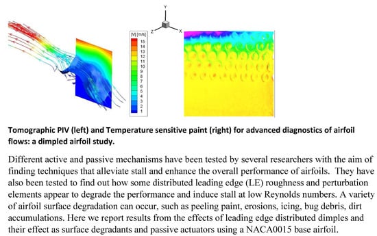
Aerodynamic stall causes abrupt decrease in lift and increase in drag, which often leads to unfavorable static or dynamic loading conditions for low-Reynolds-number airfoils. Different active and passive mechanisms have been tested by several researchers with the aim of finding techniques that alleviate stall and enhance the overall performance of airfoils. They have also been tested to determine how some distributed leading edge (LE) roughness and perturbation elements appear to degrade the performance and induce stall at low Reynolds numbers [1,2]. A variety of airfoil surface degradation can occur, such as peeling paint, erosions, icing, bug debris, dirt accumulations, protective barrier coating peeling, etc., depending on the application, degradation inevitably occurs over long-term airfoil operation. If degradations are sufficiently large in size, they may cause significant power loss, as previously reported in many investigations [1,2]. On the other hand, similar degradation elements, either passive or active, can lead to improved airfoil performance. For instance, active control mechanisms, such as dynamic pitch control [3], plasma actuators [4], and synthetic jets [5,6], have been demonstrated effective in stall control, which enhances airfoil lift generation under large incident angles and therefore increases the overall power production of the rotor blades. This improvement is largely related to the suppression of flow separation under larger angles of attack (AoA) scenarios. However, the active methods are typically not cost-effective and require relatively complicated materials and structures. Hence, the passive method of delaying stall is another important method that requires further investigation. It has been found that passive mechanisms/structures can alter the aerodynamics of airfoils substantially. Vortex generators and elevated wire on top of the LE were found to improve the post-stall behaviors of a pitching NACA0021 airfoil [7]. Large single-row disturbance generators significantly improved the performance of a pitching OA209 airfoil by delaying stall angle up to five degrees [8]. Meanwhile, research has demonstrated that introducing VGs at the mid-chord locations on the suction side can delay stall to various extents [9,10].
Although a substantial amount of work has been conducted on effects of these simple passive mechanisms on the suction side flow separation, it is still unclear and debatable how large distributed elements on the LE affect the aerodynamics at high AoA. In fact, the effects of distributed LE structures would have important implications in the real-life operation. Effects of geometry, thickness [11], and size [1,2] of the LE disturbances have been reported. Distributed at the LE, these structures may stabilize [12], modify, or intensify [13] the growth of the Tollmien-Schlichting (T-S) wave, leading to delayed or advanced transition from laminar flow to turbulence. It is also unknown whether certain passive flow control methods, such as distributed dimples used on golf ball surfaces (which includes spin and induced Magnus force features), would help prevent stall at large AoA. A number of passive and active methods have attempted to minimize the stalls.
To fill these gaps, we investigated the effects of three different types of distributed leading-edge elements, including dimples, bumps, and two-dimensional (2D) bumps on the stall behavior of a stationary NACA0015 [2]. There we performed standard planar particle image velocimetry (PIV) to investigate the stall AoA’s and the flow field variations among different models. Standard 2D PIV is most common and the simplest to set up, but it provides velocity components in only two directions. Here, we focused our study on the effects of a dimple configuration on LE that produce abrupt stall at a certain AoA using 3D flow and surface measurement techniques as explained in the following.
In an attempt to better understand the three-dimensionality (3D) of complex flows and obtain the third velocity component, a variety of techniques have been devised [14]. Examples include stereoscopic PIV, tomographic PIV, holographic PIV, dual-plane PIV, and curved laser sheet methods [15]. Most of the abovementioned techniques require specialized calibration or image correlation methods beyond those typically used for 2D single plane PIV. In the present investigation, two- and four-camera tomographic PIV [16,17,18,19] was used to obtain PIV data and gather details of boundary layer, flow separation, and near-surface flows for a dimpled configuration. The data were complemented by the temperature sensitive paint (TSP) [20,21] measurements, which provided a quantitative measurement of the separation regions and turbulence levels in LE and within the dimple regions.
2. Experimental Setup
In this study, models used in our previous investigation [2] with smooth and dimpled LE surface conditions (Figure 1) were tested. Both models had the same basic geometry of NACA0015 with a chord length c = 135 mm. A smooth airfoil was used as a baseline (referred to as “smooth”). On the second model, hemispherical cuts into the surface (referred to as “dimples”) were evenly distributed on the 20% chord of the LE of a NACA0015 with a staggered pattern. These dimples had a diameter d = 5 mm and a depth h = 2.5 mm, resulting in a roughness depth to chord ratio h/c = 0.0185. Both models were precisely fabricated using 3D printers with acrylonitrile butadiene styrene (ABS) plastic material. They were printed in two symmetrical halves and glued together. The model surfaces were carefully polished and treated with acetone vapor to remove spurious features and LE gaps.
In the present study, experiments were conducted in a low-speed, open-circuit wind tunnel with a 0.3 m × 0.3 m square test section. The models were fixed to a support structure with a geared dial system to accurately change the AoA. The models were tested under same wind speed conditions, namely ~10 m/s, resulting in Reynolds number of ~100,000 based on c. Measurements were done at incrementally increased AoA to find the angle at which separation happens for each model. Tomographic PIV and TSP were set up to conduct the near-wall and 3D flow structure study to characterize and understand the physics of the flow behavior. The setup and measurement techniques will be discussed next.
As with PIV designs, the combination of laser-sheet thickness and the time between the two frames should be such that particles do not move out of the laser sheet. Often, the focus of studies on transitional flow around airfoils is on the flow behavior in the viscous region near the wall. The walls are curved in shape and attached laminar, transitional, and turbulent boundary layer streamlines primarily follow the shape of the curved wall. Curved walls make it difficult to use traditional PIV in the spanwise viewing direction near the wall. Several researchers [22,23] have successfully applied 2D planar PIV in the spanwise direction plane parallel to the suction side of an airfoil (or flat plate with adverse pressure gradient [24]) by taking advantage of the low curvature of the blade in the region of interest. Curved laser-sheet PIV has been reported as well [2,15]. It has also been obtained by spanwise scanning PIV near the wall and through a separation bubble on the suction side of a SD7003 airfoil at Reynolds numbers of 2.0 × 10⁴ − 6.0 × 10⁴ [22].
To better capture the inherent three-dimensional nature of the flow around a dimpled system, the 3D measurements were designed to yield data near the wall. Surfaces were painted with flat black to minimize extraneous laser-light reflections and the center illuminated by the laser (green—532 nm) was painted red to further minimize the direct reflection onto the camera. Two- and four-camera tomographic PIV systems were set up in the experiments in that progression to allow for the acquisition of more data. In general, a higher number of cameras allows for more thickness of the interrogation volume, more seeding, more resolution, and more accuracy of the measurements [18]. Figure 2 and Figure 3 show the schematic of the principles and photography of the setup.
In the tomographic system, in order to test the 3D dimpled and smooth NACA 0015 airfoils, the airfoils were attached inside the wind tunnel by means of a bracket connected to the underside of the airfoil. The rod connecting to the bracket exited the wind tunnel on the bottom side and was capable of altering the angle of attack. Each airfoil was tested with the wind tunnel, producing a freestream velocity of about 10 m/s and at AoA of 10°, 12°, and 15°. The system consisted of the dual-head laser (NewWave MiniLase-III Nd:YAG, Sunnyvale, CA, USA) capable of ~100mJ/pulse and 15 Hz repetition rate and a combination of PIV cameras and adjustable Scheimpflug adapters from La Vision (Göttingen, Germany). Two cameras were Imager Intense LaVision Models with 1376 × 1040 pixels and two cameras were LaVision Imager LX GigE Models with 1608 × 1208 pixels. The two sets of cameras and lasers were synchronized with an external delay generator (ISSI PDG-2, Dayton, OH, USA) and one ‘PTU’ from LaVision. A dual-plane, dual-sided calibration target for 3D measurements with dimensions 204 × 204 mm from LaVision (model 106-10, Göttingen, Germany) was used for the calibration. The calibration, data acquisition, image processing, and data processing (volume self-calibration, 3D reconstruction, MART algorithm, etc.) [16,17,18,19] were performed with the Flow Master DaVis 8 (LaVision) software (v.8) supporting two and four cameras.
In order to record data for a volume, the laser sheet was widened to about 10 mm with the use of a cylindrical lens before being projected onto the top surface of the airfoil through a rectangular aperture to illuminate a parallel sided volume, which is a critical adjustment to obtain accurate measurements. The laser sheet was also oriented so that it would cross through the center of three rows of dimples and partially through the remaining two rows. To allow accurate reconstruction, the four cameras were placed on one side of the wind tunnel. Figure 3 displays the location of each camera with respect to an airfoil at zero degrees.
After aligning the laser and cameras for ideal volume reconstruction, the cameras were calibrated using LaVision’s calibration plate. The plate contained two surfaces to allow for three-dimensional calibration with calibration dots of 2.5 mm in diameter and 10 mm distance vertically and horizontally from other calibration dots. All four cameras were calibrated at the same time with the center of the two calibration planes in the middle of projected laser volume. After that, the software proceeded to locate the calibration dots for each camera and configure the volume reconstruction steps.
The seeding of the air during testing was acquired by dispersing atomized ‘DEHS’ oil (submicron sizes) into the inlet corresponding only to the location of the laser volume being projected. This reduced the amount of noise the cameras captured due to laser reflection of the airfoil and wind tunnel surfaces. The data was taken using two computer configurations, with each computer controlling two cameras. Both computers along with the laser were triggered using the external triggering system referred to above. After collecting simultaneous data from both computers, the data was merged correlating matching data based on individual images reviewed. Before processing the data, the original calibration was corrected using LaVision Davis’s self-calibration process. The maximum number of particles that were used to calculate the peak density was 500,000. The volume was reconstructed using the max x and y ranges and a z range of −3 mm to 3 mm. The allowed triangulation error that was calculated and used was 1.5 pixels. The calibration was set to create 8 x and y subvolumes with 4 z subvolumes. To correct for outlining calibration vectors, vector processing was performed on the self-calibration before applying the new calibration. The default “Universal outlier detection/removal/insertion” setting was used along with smoothing 3 × 3 × 3 at a multiplication of 1× and a strength of 0.5. To ensure the entire image was corrected, all the subvolumes were filled up. To ensure the new calibration did not need to be corrected again, self-calibration was performed again. Before applying the calibration, the new calibration vectors were found to be insignificant in magnitude and were aligned in the same direction. Therefore, it was determined that the self-calibration did not need to be continually performed after the first process. Once the calibration was finalized, the data for each airfoil and AoA was processed using the following order of processes: Image preprocessing, volume reconstruction, volume correlation, vector postprocessing, 3D rendering, and vector statistics. The image preprocessing utilized several settings to reduce the ghost intensity in the raw images, along with magnifying the max image intensity to about 64k. For each airfoil and AoA, a different mask was applied to remove any area that did not have the laser volume creating direct illumination. The volume reconstruction was set to construct the volume with the same settings used in the self-calibration by applying the max x and y dimensions and with the z dimension of −3 mm to 3 mm. The volume correlation used four correlation window sizes starting from a voxel size of 96 to 48, with each step using an overlap percentage of 75%. The peak search radius and volume binning was set to start at 8. Neither of the correlation volume or multi-pass postprocessing subsettings were used. The vector postprocessing 3D settings were set to the same used for the volume self-calibration. However, in this case, not all the voxels were filled up. Using the average velocity magnitude setting in the vector statistics process accommodated for the lack of completely filled planes from the previous process. This allowed for a clean reconstruction of the air flow visualized by the entire data set. Masking was applied to the areas without laser illumination, such as the pressure side underneath the airfoil.
Temperature sensitive paint (TSP) [20,21] was set up to perform surface measurements in the LE region. TSP can give accurate measurements of the separation regions due to the differences in heat transfer in the attached and separated flow regions. A replica of the 3D printed airfoil was spraypainted with TSP paint (UniTemp, ISSI Inc., Dayton, OH, USA) [21] and reference images with no flow (‘wind-off’) and no light (‘background’) were taken. Then, the model was heated ~10 degrees above the room temperature the wind tunnel was run to obtain a ‘wind-on’ image and capture those differences. The illumination source was a LED light source (ISSI LM2X-DM-400, Dayton, OH, USA), which provided 400 nm wavelength for paint excitation. The LED was pulsed and synchronized with the TSP camera (a 1.9 Mpix color camera with GigE connectivity, ISSI PSP-CCD-C, Dayton, OH, USA) using the pulse delay generator PDG-2 (ISSI, Dayton, OH, USA). Images were acquired with pulse durations ~400 ms and were averaged and processed using the ‘ProAcquire’ and ‘ProImage’ software (v.3.1), respectively (ISSI) [21]. The processing typically includes background subtraction, generation of markers for image alignments, filtering, calculating the ratio between wind-off and wind-on images, and conversion to temperature using a calibration file for the paint. Figure 4 shows a schematic and photography of the current TSP setup.
3. Results and Discussion
At low Reynolds numbers and AoA, it is often recognized that a “separation bubble promotes laminar to turbulent flow transition at the leading edge, facilitates the turbulent layer reattachment, and contributes to the high lift of a low-Reynolds-number airfoil” [22,23,24]. The “burst” of separation bubble (abrupt separation) at high AoA is the reason of a sharp decrease in lift and increase in drag for a leading-edge type stall. As the Reynolds number and AoA increase, the reattachment does not occur. As a basic symmetrical airfoil, NACA0015 resembles these features at low Reynolds number conditions. Since it has been extensively studied for various research purposes, a large database of analytical, numerical, and experimental research [25] exists very close to our current conditions. At Re ≈ 100,000, maximum lift is reached at about 15 degrees. After that, a sharp decrease in lift and increase in drag occurs, indicating the occurrence of the aerodynamic stall. These features are well-captured in PIV measurements [1,2]. Figure 5 shows results for the averaged velocity field over the smooth baseline model and the dimpled model for pre-stall and post-stall angles from our previous investigation [2]. In that study, it was found that the flow remains well-attached to the suction side until the AoA reaches above 15 degrees. The change between 15 degrees and 16 degrees is significant, indicating a LE-type separation. At 16 degrees, the flow directly detached from high curvature of the leading edge, causing a large slope in the ensuing shear layer.
The existence of LE elements/structures are found to have significant impact on the stall angle, as well as the mechanisms of the stall. As shown in Figure 5 [2], the distributed three-dimensional dimples actually slightly advance the stall (~1 degree) at Re = 100,000, relative to the baseline model. Meanwhile, the dramatic change between 14 degrees and 15 degrees and the large slope of the separated shear layer resemble the features shown in the smooth case, indicating a LE-type stall even though the dimple disturbances have been introduced. However, the thickness of the separated shear layer is obviously greater than that of the smooth case, which can be seen already by comparing Figure 5a,b, which will be discussed next. This is caused by a wandering shear layer in the dimple case as a result of disturbance-induced instability.
Due to the 3D nature of the dimple, the flow has inherent three-dimensionality [26,27,28,29] and the standard 2D PIV only provides a limited information of the boundary-layer flow. Depending on the Reynolds number and the dimple dimensions and configurations, various investigations [26,27,28,29] have reported a variety of vortical structures within the dimple cavity that contributed to the boundary layer disruption, separation, recirculation patterns, and a decreased drag in turbulent boundary layers. At low Reynolds numbers, the flow streamlines become curved on the dimple region, and the flow separates near the LE of the dimple and forms a recirculation zone before reattaching [26,27]. This investigation, initiated in [2], was undertaken to provide a global 3D study to investigate how these LE disturbances would affect global characteristics, such as leading edge phenomena and the stall process.
Results pertaining to the larger field of view showing global flow trends and velocity information in 3D are reported in the following. Data are presented with averaged and instantaneous properties including velocity vectors, streamlines, vorticity, and iso-surfaces. The 3D representation includes three planes and iso-surfaces covering the center and the sides of dimple spanwise extensions. The averaged flow field was taken from ~100 image pairs and the break-ups in the streamline continuity are due to three-dimensionality. In Figure 6, for reference, the average vector field is shown superimposed to a sample raw image background (from one of the cameras perspectives) at the center plane for 12-degree AoA (a) and 15-degree AoA (b). Vector fields and streamlines here are the result of applying a convective velocity subtraction to the vector field to emphasize the recirculation in the separation region. The noted red reflection on the airfoil surface indicates the laser-sheet thickness and location and the dimple coverage in the study (~9 mm).
The baseline smooth airfoil and the dimpled airfoil results for three depth z-planes are shown in Figure 7 and Figure 8, respectively, with streamlines on contours of velocity background for the two angles of attack. Two main findings from this data are related to the symmetry in both sides of the dimples and the notable disruption of the flow these LE dimples produce. First, in this global view, the three planes shown display minor differences, indicating symmetry. Second, and at the same time, they show the apparent influence of the dimples with respect to the smooth baseline. Besides the compression bubble in the LE of the airfoils, the dimple pattern generates transitional/turbulent bubbles in the dimple location. It is also apparent that the flow pattern before the separation region is quite different for the smooth and the dimpled cases. The dimple case obviously offers a much abrupter separation. This is evidence of dimple influence in boundary layer pattern. These mechanisms could be related to the particular staggerd pattern and depth of the dimples. Exploration of boundary layer pattern and disruption mechanisms would need be investigated using a closer view on the dimple cavity and for several dimple characteristics such as staggering pattern and dimple sizes such as those studies on flat surfaces [26,27,28,29]. However, this is beyond the scope of this real airfoil application investigation.
A large unsteady flow can be expected in these cases, especially with the large separation regions that occur during stall at the 15-degree AoA. A further interrogation of instantaneous instances produced plots such as those shown in Figure 9. These not only show evidence of three-dimensionality in the separation region, but again provide a continuous view of the depth of the flow in the spanwise (z direction), where similar flow features can be traced in each plane as a result of the tomographic reconstruction algortihms. For example, the regions of speed change, shear-layer structures, and recirculation-region patterns are readily captured in each plane. These features are washed out in the averged flow field plots, although Figure 10 shows a clean average pattern of the observed separation and the transitional/turbulent bubble pattern through the dimples past the LE.
The footprint of vortices in the shear layer and the separation and recirculating regions can be better tracked using vorticity fields and streamlines. This is shown in Figure 11 for the center plane (z = 0 mm) by comparing the instantaneous and average vorticity fields overlapped with streamlines. Vorticity is an invariant (independent of frame of reference), while the streamlines are result of the velocity field reference frame. Here, the streamlines were drawn from the velocity field after a convective velocity was subtracted. This allows visualizing the separation and recirculation regions and individual vortices from the shear layer and from dimples that are moving at that convective speed. Note that given the relatively low thickness of the volume reconstructed in this case, the iso-spanwise vorticity is plotted rather than a 3D vorticity. It should be noted that since vorticity uncertainty is higher than velocity, quantities derived from vorticity (e.g., vortex size and strength) yield higher uncertainties in the results than those from velocity and streamlines.
In order to gather some insight into the LE 3D flow structure, 3D iso-surfaces were reconstructed and are shown in various forms in Figure 12 and Figure 13. The iso-surfaces shown have two surfaces created: The first with the velocity magnitude zero, and the second iso-surface when velocity magnitude is equal to about 6 m/s. The first iso-surface helps to show the location of the airfoil. The figures show that the flow stays reattached at a minimum velocity of 6 m/s and that flow reversal can occur and result in the flow reversal entering back into the flow at a velocity of up to 6 m/s. Also, it is noteworthy that the streamlines which are not in the flow reversal move from the front–right of the image (z = 3mm) to the back–left (z = −3mm) by the time they exit the data reconstruction. However, the flow reversal starts in the front–left (z = 3 mm) and ends in the back–left (z = −3 mm). This means that the flow reversal re-enters the flow at the same location, but the beginning occurs from a different location than directly behind the ending location. This means there is some z-directional vorticity occurring in the flow reversal compared to the freestream flow.
A 3D vector plot reconstruction is also shown (Figure 14) with evidence of 3D motion within the volume, thereby demonstrating the usefulness and advantage of the tomographic technique. This plot highlights the fact that each plane has its own characteristics as reflected in the various 2D slices. It then follows that the averaged flow fields washed out much of these transversal (spanwise) variations.
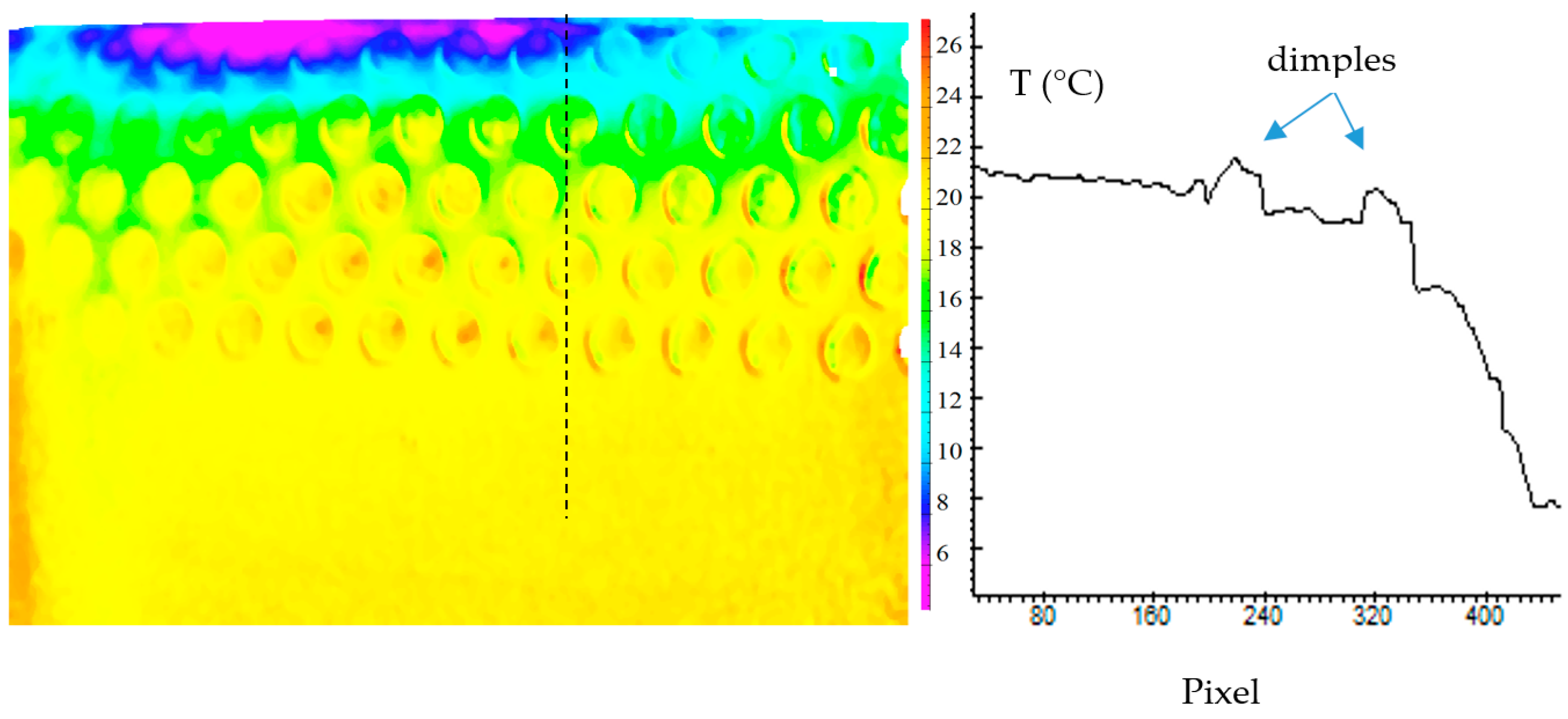
The complementary test using the TSP was performed on the dimpled airfoil and is shown next. Data acquisition comprised 128 images per run and the averaging was of 64 frames. An averaged TSP sample image for the 15-degree AoA case of the dimpled airfoil is shown in Figure 15, along with a line profile corresponding to the dashed vertical line shown on the TSP reconstructed image. The image of temperature (in °C) shows the change in intensity occurring in the LE area toward downstream, indicating separation after the second row of dimples. This is consistent with the velocity flow field obtained from PIV measurements. It is noteworthy that the TSP map and line profile show hotter regions inside the dimples, indicating higher temperature and heat transfer, thereby indicating higher transition/turbulence regions consistent with flows in cavities where recirculation and separation often occurs [26,27,28,29]. It also shows the airfoil spanwise surface temperature variation.
The TSP algorithms were corrected for illumination, paint thickness, and concentration variations to yield an accurate map [20,21]. A trend can be detected from this data that clearly exposes the fact that some dimples (individually or by given rows) have distinct features or even geometric characteristics. These produce variations in high-turbulence locations and some centers show more turbulence than others. Some of these can be traced back to imperfections and variations in the 3D printing quality which should be improved. In spite of that, the fact that dimpled surface and finish is irregular offers the opportunity to study flow over airfoil degradation patterns that are common in practice. Clearly, a study focusing on a zoom-in section of this airfoil would reveal details of the flow characteristics like those seen in numerical simulations and close-up experiments on dimpled surfaces.
4. Conclusions and Recommendations
An experimental study has been performed to study the flow separation and stall behavior of a dimple configuration in the leading edge of a NACA0015 airfoil. Compared with a baseline smooth airfoil case, distributed hemispherical dimples (h/c = −0.0185) extending from the leading edge (LE) point to 20% of the chord length were studied to assess the effects of airfoil surface degradation that would inevitably occur over long-term airfoil operation. The efficacy of the configuration was also studied using passive flow control methods. If degradations are sufficiently large in size (e.g., k/c ≥ 0.0185 in the present study), these degradations may cause significant power loss as previously reported in many field investigations. The investigation provided information on the separation structures that explain some of these phenomena. Used as passive flow control methods, dimples, however, would not prevent separation if distributed on 20% of the LE according to the current results. It is worthwhile to further investigate whether these dimples would help improve stall if placed on other locations or under other regimes, as suggested by favorable results of previous vortex generator research.
Tomographic PIV combined with TSP surface measurements provided new information and a better understanding of the effects and the underlying physics. They showed the presence of transitional/turbulent bubbles in the vicinity and within the dimples. Significant differences were observed between the smooth and the dimpled airfoil, including their attachment and separation patterns in the leading edge.
Additional 3D and TSP measurements very close to the dimple regions using close-up views would provide further insight into the global flow dynamics and the local dimple flow, vorticity field, vortex structures, and their effects and interactions with the main flow and shear layer. Improving the four-camera arrangements and further reducing airfoil laser reflection (e.g., using a different angle setup for the cameras) could allow to gather higher resolution and higher accuracy data near the wall. Some 3D printing improvements would also make the models roughness and the LE more uniform. Nonetheless, an irregular surface is also of interest for mimicking real airfoil degradation.
The inclusion of more laminar and turbulent Reynolds numbers and other configurations including cambered airfoils would provide additional information for various regimes and efficacy for passive control performance. The addition of time-resolved capabilities (high-repetition-rate PIV systems) would allow study transients and the effects of the dimples and other structures in moving airfoils and in flapping, flutter, and spinning phenomena at various frequencies. This would allow the assessment of other effects of flow and vortex motions on the airfoil.
Author Contributions
Formal analysis, A.J.S., A.H.U. and J.E.; Writing—original draft, A.J.S., A.H.U. and J.E.
Funding
This research received no external funding.
Conflicts of Interest
The authors declare no conflict of interest.
Nomenclature
| α, AoA | = angle of attack |
| CL | = lift coefficient |
| c | = chord |
| d | = dimple diameter |
| h | = dimple depth |
| LE | = leading edge |
| M | = magnification |
| PIV | = particle image velocimetry |
| Re | = Reynolds number |
| TSP | = temperature sensitive paint |
| u | = velocity component in x direction |
| v | = velocity component in y direction |
| V | = velocity magnitude |
| x | = main-flow direction |
| y | =surface normal direction |
| z | = spanwise direction |
References
- Zhang, Y.; Igarashi, T.; Hu, H. Experimental Investigations on the Performance Degradation of a Low-Reynolds-Number Airfoil with ith Distributed Leading Edge Roughness. In Proceedings of the 49th AIAA Aerospace Sciences Meeting including the New Horizons Forum and Aerospace Exposition, Orlando, FL, USA, 4–7 January 2011. [Google Scholar]
- Zhang, Y.; Estevadeordal, J.; Bhusal, S.; Krech, J. Effects of Leading-Edge Structures on Stall Behaviors of a NACA0015 Airfoil: A Multi-plane PIV Study. In Proceedings of the 34th AIAA Applied Aerodynamics Conference, Washington, DC, USA, 13–17 June 2016. [Google Scholar]
- Hwang, I.S.; Min, S.Y.; Jeong, I.O.; Lee, Y.H.; Kim, S.J. Efficiency improvement of a new vertical axis wind turbine by individual active control of blade motion. In Proceedings of the Smart Structures and Materials 2006: Smart Structures and Integrated Systems, San Diego, CA, USA, 26 February–2 March 2006. Abstract Number: 6173, Pagination: 617311. [Google Scholar]
- Greenblatt, D.; Schulman, M.; Ben-Harav, A. Vertical axis wind turbine performance enhancement using plasma actuators. Renew. Energy 2012, 37, 345–354. [Google Scholar] [CrossRef]
- Sasson, B.; Greenblatt, D. Effect of Leading-Edge Slot Blowing on a Vertical Axis Wind Turbine. AIAA J. 2011, 49, 1932–1942. [Google Scholar] [CrossRef]
- Yen, J.; Ahmed, N.A. Enhancing vertical axis wind turbine by dynamic stall control using synthetic jets. J. Wind. Eng. Ind. Aerodyn. 2013, 114, 12–17. [Google Scholar] [CrossRef]
- Choudhry, A.; Arjomandi, M.; Kelso, R. Methods to control dynamic stall for wind turbine applications. Renew. Energy 2016, 86, 26–37. [Google Scholar] [CrossRef]
- Heine, B.; Mulleners, K.; Joubert, G.; Raffel, M. Dynamic Stall Control by Passive Disturbance Generators. AIAA J. 2013, 51, 2086–2097. [Google Scholar] [CrossRef] [Green Version]
- McCullough, G.B.; Gault, D.E. Examples of Three Representatine Types of Airfoil-Section Stall at Low Speed; NACA Technical Note 2502; National Advisory Committee for Aeronautics: Moffett Field, CA, USA, 1951; p. 263.
- Shan, H.; Jiang, L.; Liu, C.; Love, M.; Maines, B. Numerical study of passive and active flow separation control over a NACA0012 airfoil. Comput. Fluids 2008, 37, 975–992. [Google Scholar] [CrossRef]
- Li, Y.; Tagawa, K.; Liu, W. Performance effects of attachment on blade on a straight-bladed vertical axis wind turbine. Curr. Appl. Phys. 2010, 10, S335–S338. [Google Scholar] [CrossRef]
- Fransson, J.H.M.; Talamelli, A.; Brandt, L.; Cossu, C. Delaying Transition to Turbulence by a Passive Mechanism. Phys. Rev. Lett. 2006, 96, 064501. [Google Scholar] [CrossRef] [PubMed] [Green Version]
- Kerho, M.F.; Bragg, M.B. Airfoil Boundary-Layer Development and Transition with Large Leading-Edge Roughness. AIAA J. 1997, 35, 75–84. [Google Scholar] [CrossRef] [Green Version]
- Raffel, M.; Willert, C.E.; Scarano, F.; Kahler, C.; Wereley, S.T.; Kompenhans, J. Particle Image Velocimetry: A Practical Guide, 3th ed.; Springer: New York, NY, USA, 2018. [Google Scholar]
- Estevadeordal, J.; Marks, C.; Sondergaard, R.; Wolff, M. Curved laser-sheet for conformal surface flow diagnostics. Exp. Fluids 2011, 50, 761–768. [Google Scholar] [CrossRef]
- Elsinga, G.E.; Scarano, F.; Wieneke, B.; Van Oudheusden, B.W. Tomographic particle image velocimetry. Exp. Fluids 2006, 41, 933–947. [Google Scholar] [CrossRef]
- Wieneke, B. Volume self-calibration for 3D particle image velocimetry. Exp. Fluids 2008, 45, 549–556. [Google Scholar] [CrossRef]
- Scarano, F. Tomographic PIV: principles and practice. Meas. Sci. Technol. 2013, 24, 1–27. [Google Scholar] [CrossRef]
- Sciacchitano, A.; Wieneke, B. PIV uncertainty propagation. Meas. Sci. Technol. 2016, 27, 084006. [Google Scholar] [CrossRef] [Green Version]
- Liu, T.; Sullivan, J.P. Pressure and Temperature Sensitive Paints; Springer: Berlin/Heidelberg, Germany, 2005. [Google Scholar]
- ISSI Inc., Pressure and Temperature Sensitive Paints. Available online: https://innssi.com/tsp/ (accessed on 1 October 2019).
- Burgmann, S.; Brücker, C.; Schröder, W. Scanning PIV measurements of a laminar separation bubble. Exp. Fluids 2006, 41, 319–326. [Google Scholar] [CrossRef]
- Zhang, W.; Hain, R.; Kähler, C.J. Scanning PIV investigation of the laminar separation bubble on a SD7003 airfoil. Exp. Fluids 2008, 45, 725–743. [Google Scholar] [CrossRef]
- Rist, U.; Lang, M.; Wagner, S. Investigations on controlled transition development in a laminar separation bubble by means of LDA and PIV. Exp. Fluids 2004, 36, 43–52. [Google Scholar] [CrossRef]
- Drela, M. XFOIL: An Analysis and Design System for Low Reynolds Number Airfoils. In Lecture Notes in Engineering; Springer Science and Business Media LLC: Berlin/Heidelberg, Germany, 1989; pp. 1–12. [Google Scholar]
- Kovalenko, G.V.; Terekhov, V.I.; Khalatov, A.A. Flow regimes in a single dimple on the channel surface. J. Appl. Mech. Tech. Phys. 2010, 51, 839–848. [Google Scholar] [CrossRef]
- Van Nesselrooij, M.; Veldhuis, L.L.M.; Van Oudheusden, B.W.; Schrijer, F.F.J. Drag reduction by means of dimpled surfaces in turbulent boundary layers. Exp. Fluids 2016, 57, 142. [Google Scholar] [CrossRef]
- Tay, J.; Lim, T.T.; Khoo, B.C. Drag Reduction with Diamond-shaped Dimples. In Proceedings of the AIAA Aviation Forum, Dallas, TX, USA, 17–21 June 2019. AIAA-2019-3296. [Google Scholar]
- Xie, Y.; Shen, Z.; Zhang, D.; Ligrani, P. Numerical Analysis of Flow Structure and Heat Transfer Characteristics in Dimpled Channels with Secondary Protrusions. J. Heat Transfer 2016, 138, 031901. [Google Scholar] [CrossRef]
- Stolt, A.; Estevadeordal, J.; Krech, J.; Zhang, Y. A tomographic PIV and TSP Study of Leading-Edge Structures on Stall Behaviors of NACA0015. In Proceedings of the 55th AIAA Aerospace Sciences Meeting, Grapevine, TX, USA, 9–13 January 2017. [Google Scholar]
Figure 1.
Test models and dimple geometry details. Adapted from Zhang et al. [2].
Figure 1.
Test models and dimple geometry details. Adapted from Zhang et al. [2].

Figure 2.
Basic process for multiple camera tomographic particle image velocimetry (PIV).
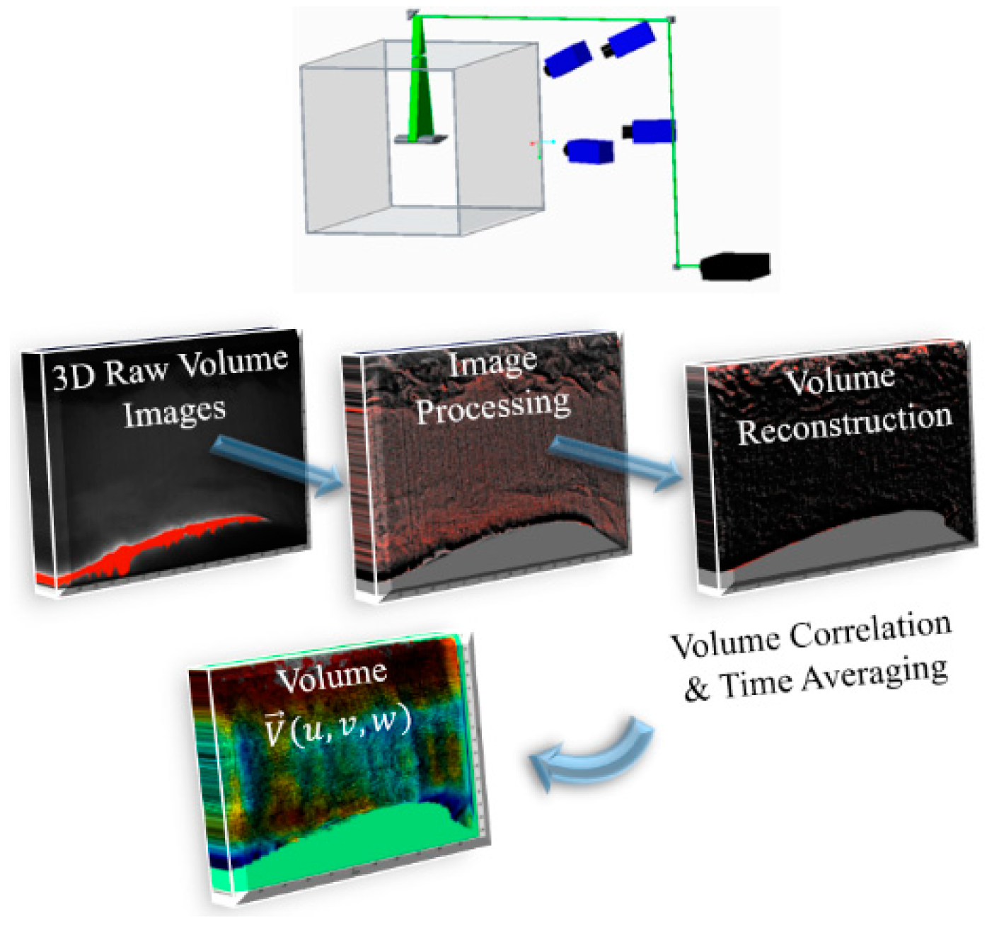
Figure 3.
Tomographic setup photography.

Figure 4.
Temperature sensitive paint (TSP) schematic (ISSI Inc.), reproduced from [21]. (a) and current North Dakota State University (NDSU) Advanced Flow Measurements Laboratory setup photography (b).
Figure 4.
Temperature sensitive paint (TSP) schematic (ISSI Inc.), reproduced from [21]. (a) and current North Dakota State University (NDSU) Advanced Flow Measurements Laboratory setup photography (b).
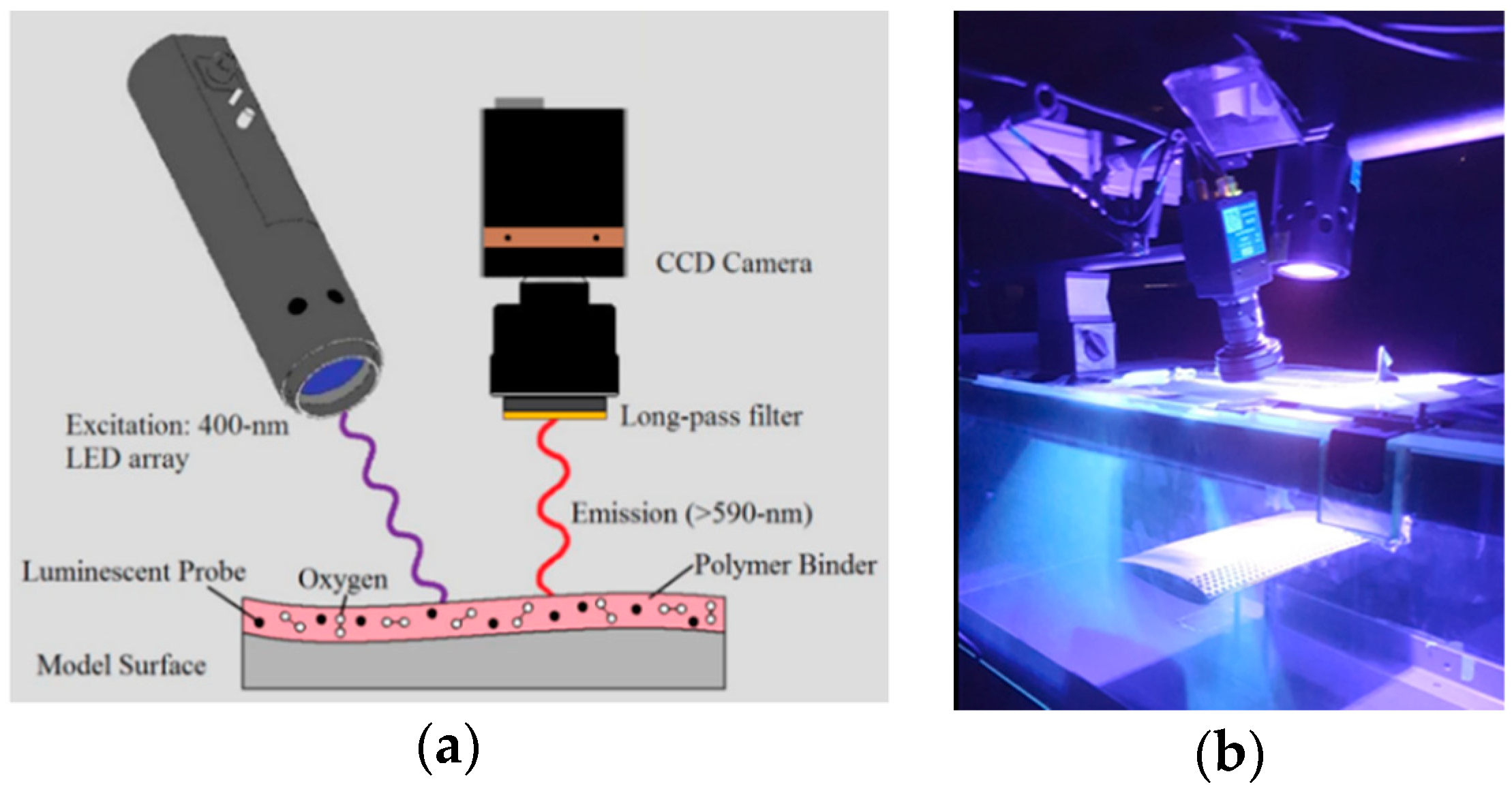
Figure 5.
Averaged velocity field at high angle of attack (AoA) for the smooth (a) and dimpled (b) airfoils. Reproduced from Zhang et al. [2].
Figure 5.
Averaged velocity field at high angle of attack (AoA) for the smooth (a) and dimpled (b) airfoils. Reproduced from Zhang et al. [2].
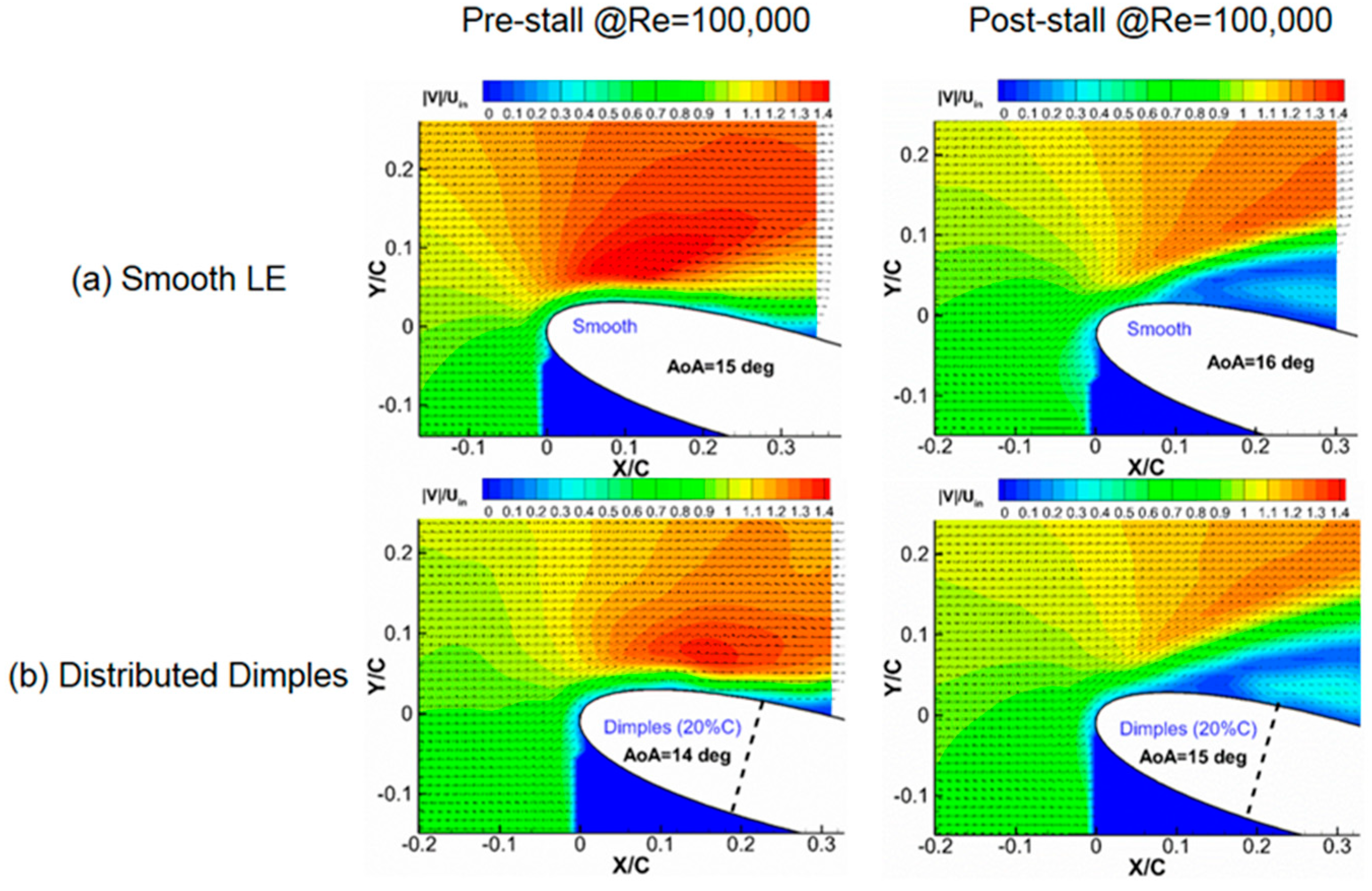
Figure 6.
Average vector field superimposed to a sample raw image background (from one of the camera perpectives) at the center plane for 12-degree AoA (a) and 15-degree AoA (b). Vector fields and streamlines are the result of applying a convective velocity subtraction to vector field. Red reflection on airfoil surface indicates the laser-sheet thickness and dimple coverage (~9 mm).
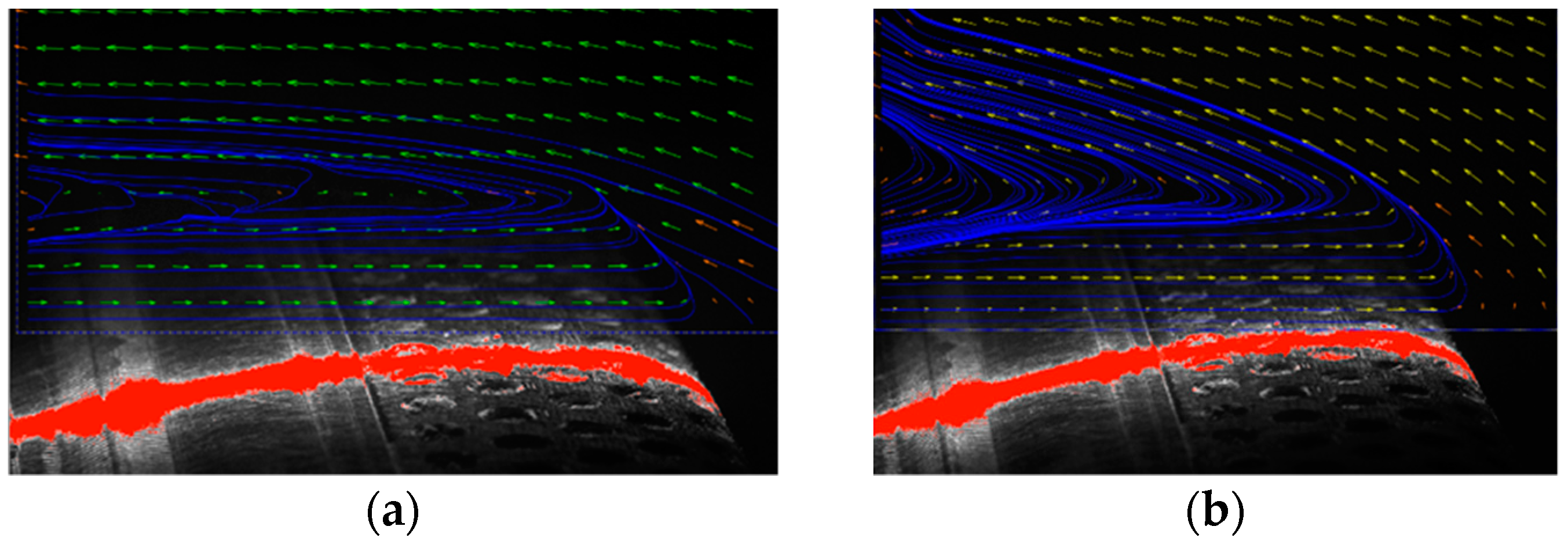
Figure 7.
Three sample planes from two-camera 3D reconstruction for the smooth airfoil at two AoA.
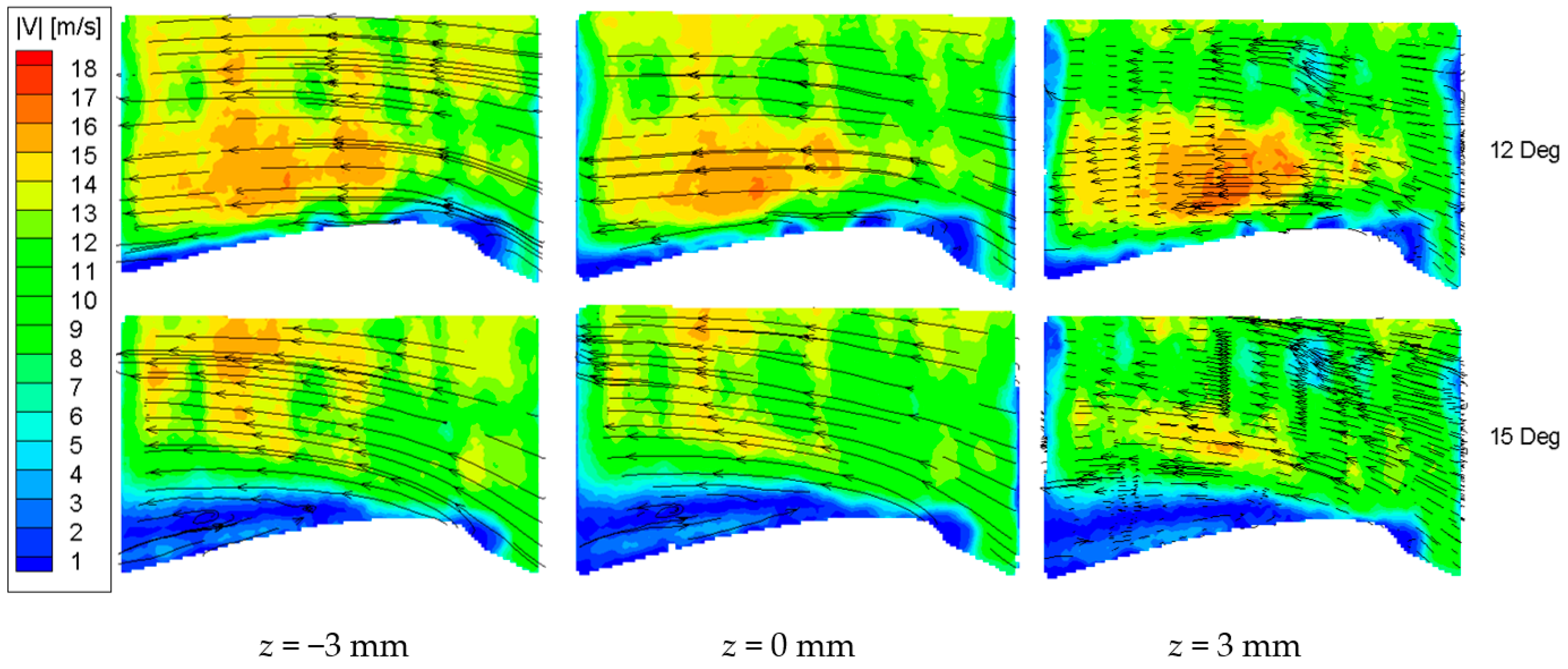
Figure 8.
Three sample planes from two-camera 3D reconstruction for the dimpled airfoil at two AoA.

Figure 9.
Instantaneous vector field with turbulent separated region for dimpled airfoil (15-degree AoA).
Figure 9.
Instantaneous vector field with turbulent separated region for dimpled airfoil (15-degree AoA).

Figure 10.
Average vector field showing turbulent bubbles formed where the dimples are located (15-degree AoA).
Figure 10.
Average vector field showing turbulent bubbles formed where the dimples are located (15-degree AoA).
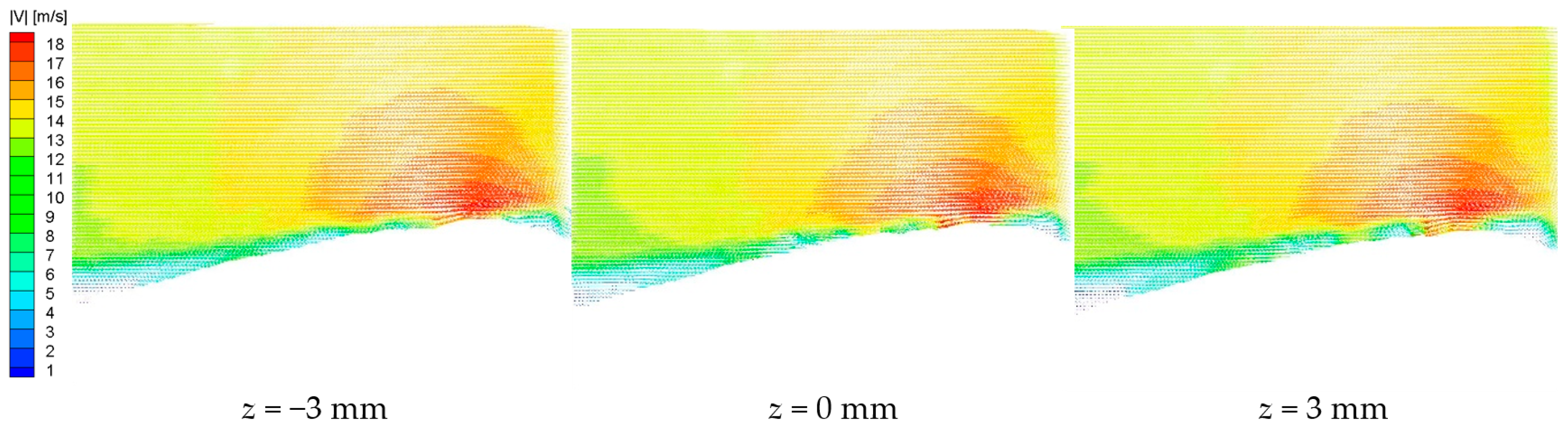
Figure 11.
Instantaneous (a) and average (b) spanwise vorticity (ωz) fields superimposed with average vector field at center plane (z = 0 mm) for 12-degree AoA (left) and 15-degree AoA (right). Vector fields and streamlines are the result from applying a convective velocity subtraction.
Figure 11.
Instantaneous (a) and average (b) spanwise vorticity (ωz) fields superimposed with average vector field at center plane (z = 0 mm) for 12-degree AoA (left) and 15-degree AoA (right). Vector fields and streamlines are the result from applying a convective velocity subtraction.
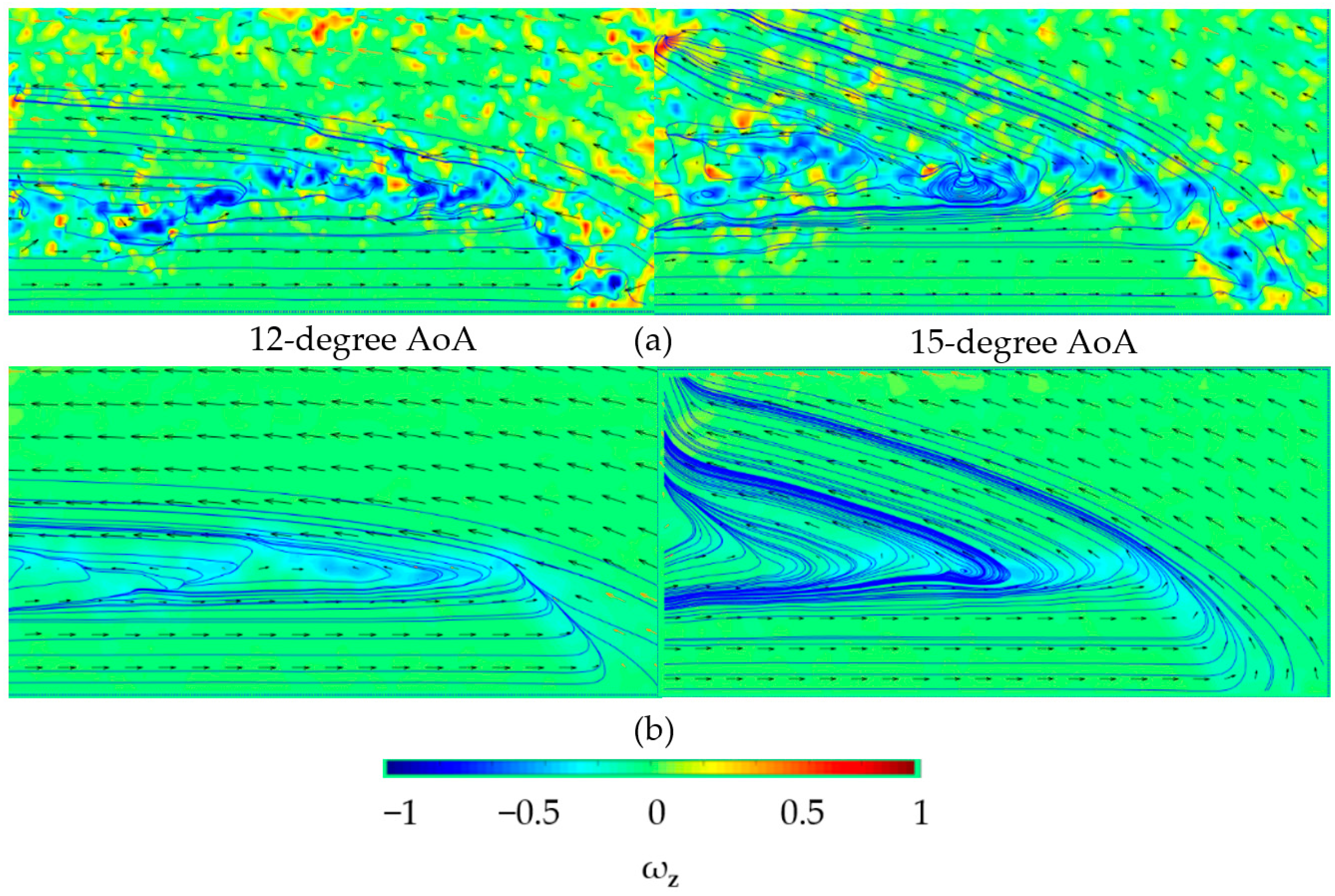
Figure 12.
Iso-surfaces and streamlines at two scale display levels. Reproduced from Stolt et al. [30].
Figure 12.
Iso-surfaces and streamlines at two scale display levels. Reproduced from Stolt et al. [30].
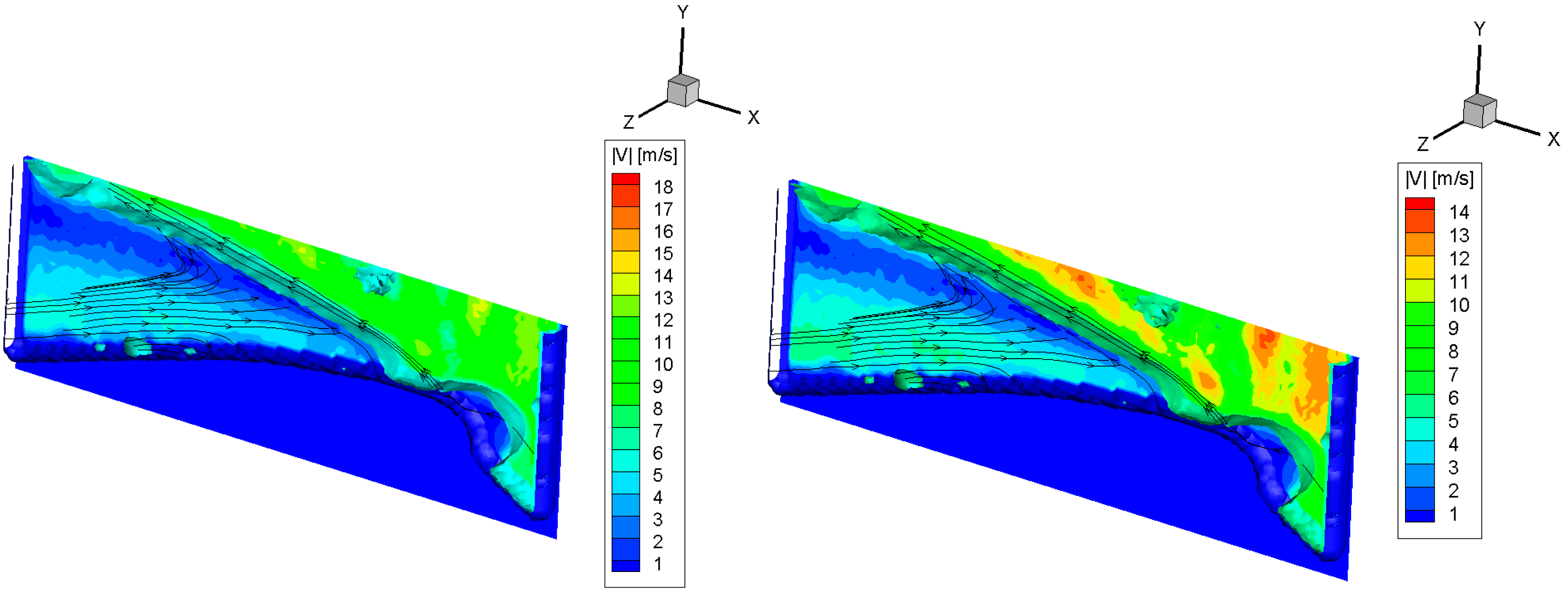
Figure 13.
Iso-surfaces and streamlines at two display formats. Reproduced from Stolt et al. [30].
Figure 13.
Iso-surfaces and streamlines at two display formats. Reproduced from Stolt et al. [30].
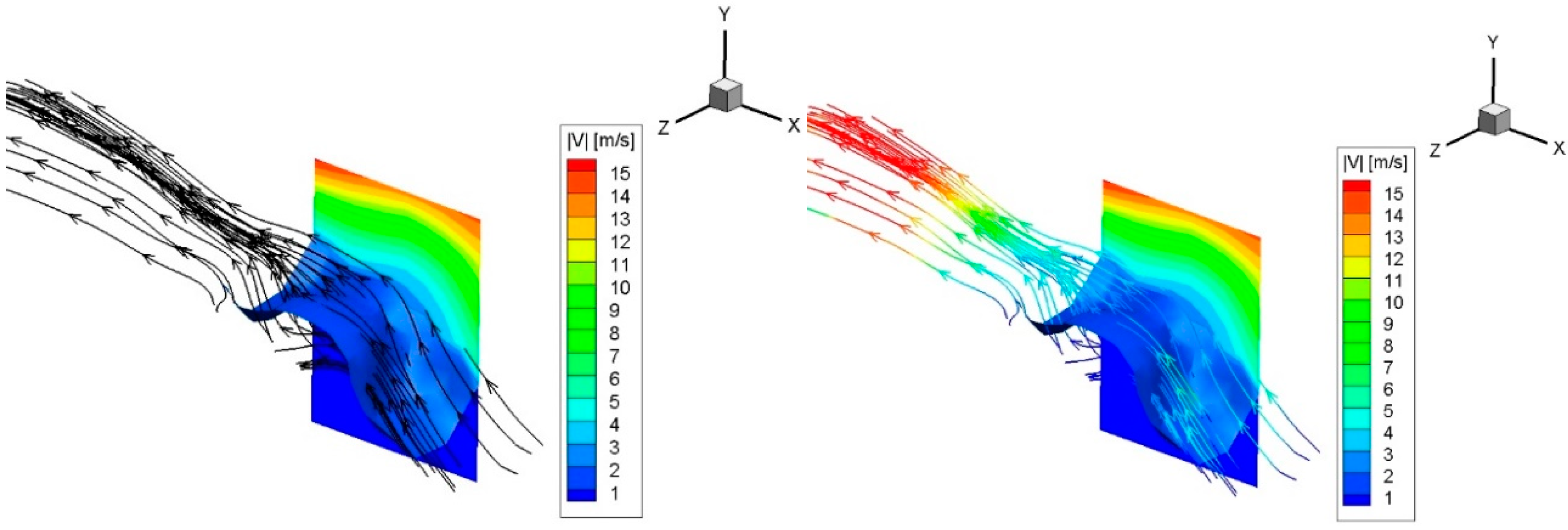
Figure 14.
Average velocity field view of the leading edge (LE) dimpled airfoil at the 15-degree AoA. Reproduced from Stolt et al. [30].
Figure 14.
Average velocity field view of the leading edge (LE) dimpled airfoil at the 15-degree AoA. Reproduced from Stolt et al. [30].
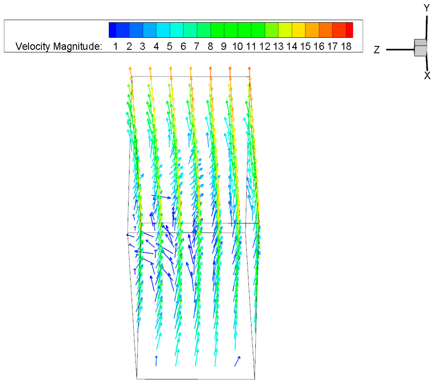
Figure 15.
Average TSP map and line profile for the dimpled airfoil at the 15-degree AoA. Reproduced from Stolt et al. [30].
Figure 15.
Average TSP map and line profile for the dimpled airfoil at the 15-degree AoA. Reproduced from Stolt et al. [30].
© 2019 by the authors. Licensee MDPI, Basel, Switzerland. This article is an open access article distributed under the terms and conditions of the Creative Commons Attribution (CC BY) license (http://creativecommons.org/licenses/by/4.0/).
Share and Cite
MDPI and ACS Style
Stolt, A.J.; Ullah, A.H.; Estevadeordal, J. Study of Leading-Edge Dimple Effects on Airfoil Flow Using Tomographic PIV and Temperature Sensitive Paint. Fluids 2019, 4, 184. https://doi.org/10.3390/fluids4040184
AMA Style
Stolt AJ, Ullah AH, Estevadeordal J. Study of Leading-Edge Dimple Effects on Airfoil Flow Using Tomographic PIV and Temperature Sensitive Paint. Fluids. 2019; 4(4):184. https://doi.org/10.3390/fluids4040184
Chicago/Turabian StyleStolt, Adam J., Al Habib Ullah, and Jordi Estevadeordal. 2019. "Study of Leading-Edge Dimple Effects on Airfoil Flow Using Tomographic PIV and Temperature Sensitive Paint" Fluids 4, no. 4: 184. https://doi.org/10.3390/fluids4040184