Experimental Measurement of Steady and Transient Liquid Coiling with High-Speed Video and Digital Image Processing

Abstract

Liquid coiling occurs as a viscous fluid flows into a stagnant reservoir causing a localized accumulation of settling material, which coils into a stack as it accumulates. These coiling flows are broadly characterized into three primary coiling regimes of viscous, gravitational, or inertial coiling, based on the velocity of the falling fluid, the height of the fall, the radius of the fluid rope, the stack height, and the fluid properties including viscosity. A computer-controlled flow delivery apparatus was developed here to produce precisely controlled flow conditions to study steady and transitional coiling regimes with independently varied parameters. Data were recorded using high-speed digital video cameras and a purpose-built digital image processing routine to extract rope and stack dimensions as well as time-resolved coiling frequency. The precision of the setup and data analysis methods allowed a detailed study of the transition between gravitational and inertial flow regimes. The results show a smooth transition between the regimes, with no evidence of the inertial-gravitational regime. Unsteady coiling was able to be momentarily produced by applying a perturbation to the system, but the unstable regime quickly decayed to either the base inertial or gravitational regime.

Dataset:https://drive.google.com/drive/folders/1kNXjOryyqkDASyPqajeBdJx3jp2XXuxp?usp=sharing

Dataset License: CC-BY-SA

1. Introduction and Liquid Coiling Regimes

Under appropriate conditions, a falling stream of viscous liquid may exhibit the phenomena of liquid coiling when encountering a quiescent reservoir of the same fluid. Deceleration of the falling liquid can cause the stream to spontaneously rotate about and accumulate into a cylindrical stack [1]. This instability is analogous to buckling of solid columns under compressive loads [2]. Differences and complexities arise as liquid continues to flow into the system and dissipates into a surrounding reservoir.

The liquid coiling phenomenon can be categorized into four different coiling regimes defined as viscous, gravitational, inertial-gravitational, and inertial. Parametric relations have been developed to describe the steady coiling frequencies for the four regimes using numerical simulations [3]. The flow regime of the coil stack is influenced by a variety of factors including fluid flow rate, kinematic viscosity, and drop height. These factors affect the general shape of the coil stack and the range of the coil dimensions. These dimensions include the tail radius, stack height, stack width, and coiling frequency as identified in Figure 1.

Numerical simulations of a viscous liquid rope identify distinct, steady coiling regimes [4]. Coiling frequency provides a quantifiable metric to identify a viscous, gravitational, and inertial coiling regime with respectively increasing coiling frequencies [5]. Extensive numerical and experimental research has been conducted to quantify the various liquid coiling regimes and to correlate numerical simulation to experimental data [6]. Experimental investigation under a constant flow rate and a variable height show good correlation with the numerical analysis [7].

Simulations and experiments show the existence of a fourth regime, the inertial-gravitational regime, which is a region of instability that occurs during the transition between the gravitational and inertial regimes [6]. However, frequency does not guarantee explicit identification of the transitional inertial-gravitational regime. This flow manifests in an unpredictable manner with rapid stack growth and collapse with variable coiling frequencies generally similar in magnitude to the gravitational and inertial regimes. Inertial-gravitational coiling is observed to be erratic in nature, and transitions have been observed following manual perturbations to the system [8]. Experimentation within the inertial-gravitational regime inherently requires a time component due to the unpredictable and varying coiling patterns [9].

Additional experimental studies with substantial quantitative models describing the underlying physics of other aspects of the liquid coiling type instabilities have been performed. Secondary buckling or supercoiling of the stack deposited by traditional liquid coiling have been investigated and systematically measured [10]. Bubble generation within the stack has been demonstrated with systematic Fermat spirals [11]. Additionally, rope coiling onto an automated moving surface has been explored, which resulted in the ability to describe coiling regimes much like those seen in classic liquid coiling [12].

Recent experiments have employed high speed imaging to view the coiling motion at frame rates exceeding 1000 fps often with a manual analysis of the images [2,7,10,13]. In older experimental work, inaccuracies in the measurement of coiling frequency due to camera limitations have resulted in the failure to experimentally record the inertial-gravitational regime in some investigations [14]. The work presented in this paper expands upon previous work by automating the analysis of image sets using image processing techniques. The image processing routines are developed to track and measure features of the coil to provide a systematic analysis that increases the repeatability of the results and the ability to interpret larger quantities of data. An automated system was also developed to produce these coiling flows with the ability to independently vary parameters of the flow with precise control. Further, this system is demonstrated under transient flow rate conditions with time-resolved measurements of coiling frequency, stack height, and stack diameter.

2. Test Apparatus Design and Calibration

2.1. Variable Syringe Pump Test Stand

A programmable syringe pump was designed and fabricated to generate precise and variable flow. The flow is driven by a stepper motor powered syringe pump allowing for the control of the flow rate. Laser cut acrylic sheets (6 mm thick) comprise the majority of the syringe pump structure and are supported by an 80/20 brand aluminum extrusion frame as visible in Figure 2a. Manual scissor lifts placed on opposite sides of the frame are utilized to vary drop height between tests. To ensure that the syringe orifice is appropriately aligned, a digital level was used to confirm the adjustment of the scissor lifts before every test to within 0.1°. The syringe pump was designed for modularity with interchangeable syringes and an 18 gauge Leur taper syringe tip. The syringe tip fixed the orifice diameter at 0.97 mm. Syringes used during testing had a 33 mL capacity that allowed for sufficient vertical travel of the syringe plunger per volume of liquid expelled to ensure flow rate accuracy. Syringes are held rigidly via the finger flange located at the top of the barrel, and the tip is supported by a height adjustable plate.

The syringe plunger is actuated by a NEMA 23 stepper motor with a threaded spindle. A push rod is securely fastened to the drive nut on the threaded spindle with an aluminum adapter block. To translate the rotary motion of the motor into a linear motion, the push rod is held irrotationally by two fixed acrylic plates with appropriately sized square cutouts. Figure 2b shows a diagram of the syringe apparatus.

A reservoir was also fabricated from laser cut acrylic to provide the stationary liquid for the coil to form on top of. Before testing, the reservoir is filled to its maximum. Overflow from testing is caught by another container placed below the reservoir. By testing with the reservoir overflowing, the liquid level on which the coil forms is consistent. This aids in the digital image processing routine. A scissor lift holds the reservoir and overflow container, but this is not adjusted for height variation but rather to place the reservoir at a desired location in the camera’s field of view. The reservoir also incorporates a focusing plate that allows for the focusing of the camera exactly at the location of the liquid coil, which is further described in Section 3.2.

2.2. System Control and Calibration

An Arduino Mega 2560 micro-controller was used for the control of the syringe pump stepper motor and camera synchronization. An A4988 stepper motor controller was used to trigger motor stepping concurrent to rising edges of a 5 V digital output pin from the Arduino. Arduino scripts were written to perform steady state and linear ramping flow rate conditions based on the time duration between motor steps. Tests were initiated by the press of a non-latching button, which would set an elapsed time variable to zero within the script. Based on the elapsed time, different ramping and holding operations can be performed with the stepper motor and correlation with camera triggering can be made. A BNC wire interface was fabricated between an Arduino output pin and the TTL trigger functionality of the Photron high-speed cameras. Once the elapsed time reaches a desired value, a signal on this pin would trigger the camera. As the Arduino controls the stepper motor and is used to determine camera triggering, each frame can be correlated with an instantaneous flow rate.

When testing near the transition between inertial and gravitational regimes, as determined by varying drop height under steady flow rate conditions discussed in Section 4.2, unsteady coiling characteristics were initiated by a physical perturbation to the system. This perturbation was performed as a single mild impact from a hammer to the aluminum frame of the syringe pump. For correlation between this event and imaging, the head of the hammer was electrified and contact with the syringe pump frame was used as a momentary switch. Upon receiving the signal of the hammer impact, the Arduino would trigger the camera similarly to other tests. The camera was configured to record at a center trigger for these trials, which provided imaging before and after the perturbation.

The time interval between two rising edges of the 5 V pulses from the Arduino to the motor controller defines the step rate of the motor and thus the flow rate through the syringe. Calibrations were performed on Arduino scripts to ensure accurate step rates. An oscilloscope was used to measure the time between rising edges, and an offset was manually programmed to calibrate the timing. The time offset is effectively an experimentally measured value correlating to the finite time for the Arduino to loop once through the script. This approach ensures that calibrations of each code script are accurate regardless of the desired motor step rate. Once step rates are calibrated, stepper motor control provides an accurate and controllable open-loop control solution for the fluid flow rate.

3. Image Recording and Analysis

3.1. Cameras and Lighting Used during Experiments

Images were recorded at a frame rate of 1 kHz to provide adequate time resolution for the coiling frequencies being measured, and a shutter speed of 10 µs allowed negligible image blur. Photron UX-100 Mini (Photron, Tokyo, Japan) and SA-X2 (Photron, Tokyo, Japan) cameras were used throughout testing with resolutions set at 1024 by 1024 pixels. The Photron SA-X2 with 64 GB of memory was only used on the variable flow rate and perturbation tests to provide a longer record time of 43.6 s, but the 4 GB memory of the UX-100 Mini was sufficient for steady-state trials, with 10.9 s of recording time. All tests were performed with the same 60 mm fixed focal length lens with an $f/4$ aperture.

A backlighting arrangement shown in Figure 2a was implemented in all tests for increased clarity and contrast in images. An array of white LEDs with a frosted plastic screen created a source of diffuse light, which appears as an even white background in images. Liquids block and refract significant amounts of light; thus, the edges of the coil appear nearly black and can be precisely imaged with minimal ambiguity due to the high contrast. The center of the liquid appears white, but this was resolved in image processing by performing a flood filling operation from the center of the tail at the top of the image.

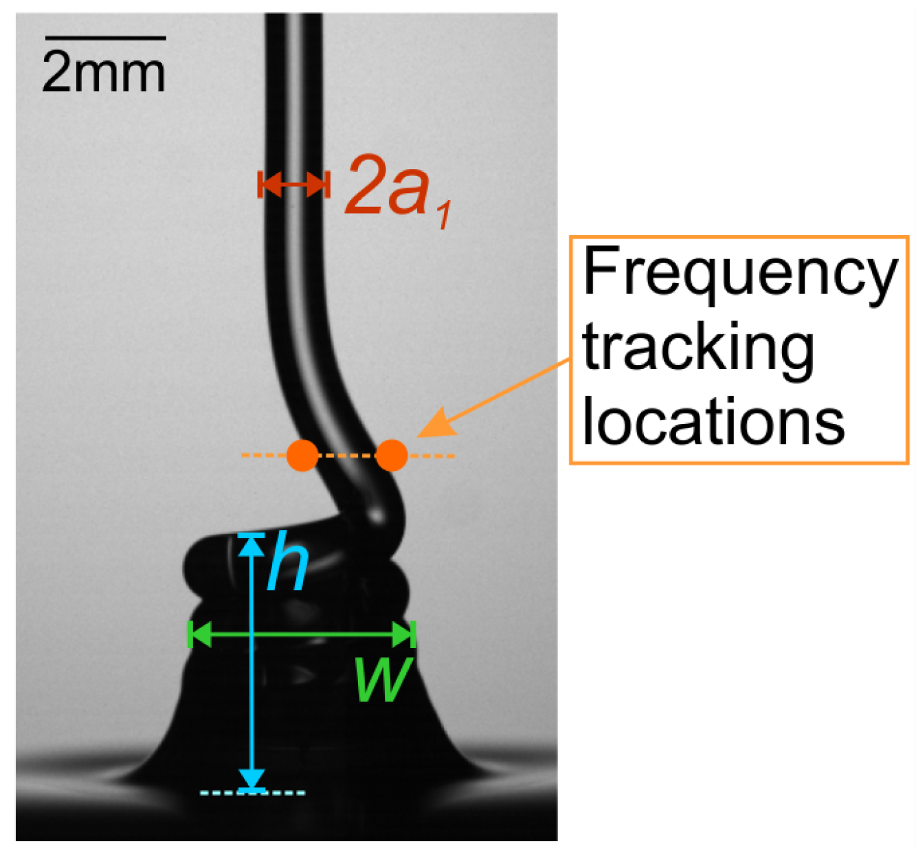
3.2. Automated Approach to Measuring Coiling Parameters from Images

MATLAB was used to process high-speed test image files. Regions of interest (ROIs) were selected by the user on the initial image to designate the tail and stack regions of the coil as shown in Figure 3. The image portions in the tail and stack ROIs were then binarized using a threshold of the average pixel intensity within the threshold ROI. The threshold ROI is the 10 × 10 array of pixel in the upper left-hand portion of an image. The resulting binarized ROIs are used for measurements where the background and coil are pure white and black, respectively.

While ROIs are manually defined once, these windows change in size with respect to the changing size of the coil stack allowing for a measurement of transient liquid coiling tests. This was done by setting a buffer region on the initial ROIs on the first image. The buffer region maintains a set pixel distance between the edges of the coil stack and the boundaries of the ROI. The ROI will extend or retract depending on the size of the current coil stack allowing for transient data analysis with fluctuating flow properties.

Tail radius, stack height, and stack width measurements are performed within the tail and stack ROIs after images are binarized. Tail radius is determined by the width of the black portion within the bottom row of pixels in the tail ROI. Measurement data along the top edge of the stack proved difficult due to the constant deposition of the liquid rope coil. Therefore, the measurement line shown in Figure 3 was set in order to determine measurements from a defined location. This line was positioned at a distance equivalent to the tail radius below the top of the coil stack, which allows for consistent measurement. Stack height was determined by measuring from this line to the bottom of the ROI at the liquid level within the reservoir. The stack width was measured as the distance between the edges of the coil stack along the measurement line.

The coiling frequency of the stack was determined by tracking the left and right edges of the depositing coil within the tail ROI throughout all test images. The sinusoidal motion of the falling rope was plotted against elapsed testing time as shown in Figure 4. The peaks of the curves were identified and the period was calculated for each full coil revolution. Frequency is simply calculated as the reciprocal of the coiling period.

A focusing object is imaged before every test which provides a conversion from pixel length to actual length. This laser-etched acrylic plate is placed in the center of the reservoir and allows for focusing and scale reference. The focusing pattern, seen in Figure 5, is of the New Mexico Tech logo and text, which gives detailed features for adjusting camera focus. Placement in the reservoir directly under the syringe orifice allows for an exact focus on the center of the coil. A 19.1 mm square is present as a scale reference, and a MATLAB code was written to measure the side length. Side length is calculated by taking the square root of the entire pixel area within the black outline of the square, allowing for a more robust measurement.

4. Steady Coiling Experiments

4.1. Demonstrating Different Flow Regimes with Honey

Honey was used here to conduct a series of steady state tests. Previous experiments have shown that honey can be used to demonstrate liquid rope coiling [13]. Viscosity was measured to be 6900 cSt with an Anton Paar MCR301 rheometer, and the honey was stored in a container within a climate-controlled facility. Experimental investigation has shown honey to be a Newtonian fluid [15].

The drop height and flow rate were incremented independently. Starting from a short drop height and high flow rate, both parameters were systematically adjusted to produce viscous, gravitational, and inertial coiling regimes. As shown in Figure 6, the different regimes are identified due to the distinctly different coiling frequencies. Coiling frequency was demonstrated to be consistent throughout each trial, and the scatter seen in the data is indicative of the measurement precision. Since each frequency datapoint is representative of the coil completing one full revolution, there is broader discretization at higher frequencies. The coil stack height remained constant during each individual steady state test. The raw stack height data was filtered using a moving average due to the small height fluctuations that occurred in measurement along a variable location.

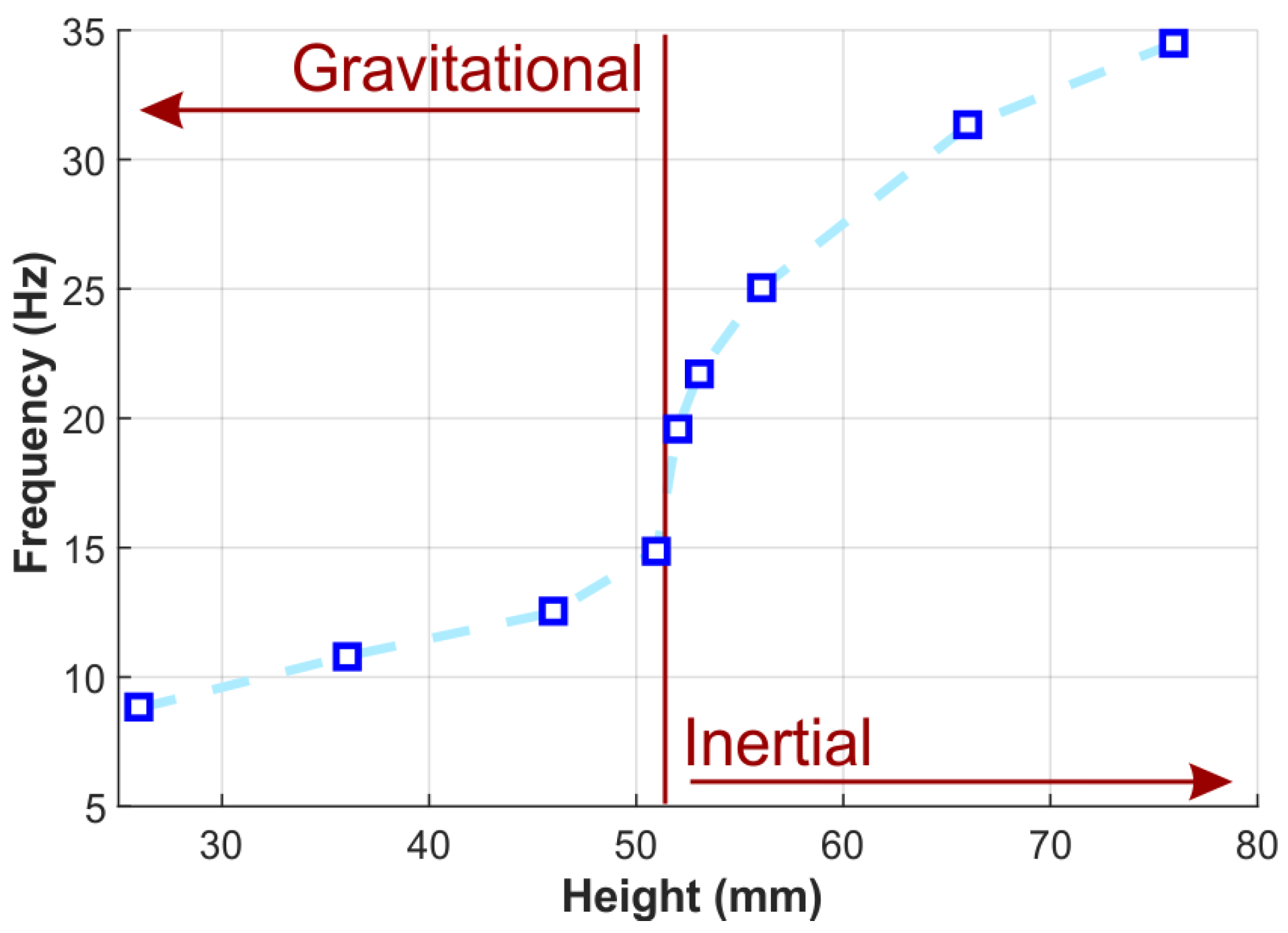
4.2. Varying Drop Height under Steady Conditions

A series of tests was performed under the steady state conditions with a fixed flow rate of 0.18 mL·s⁻¹ and various heights. The drop height was altered between individual trials. At a 26 mm drop height, coiling frequency and characteristics resembles the gravitational regime. However, at a drop height of 76 mm, the higher coiling frequency and thinning liquid tail connote an inertial flow regime. Measured frequency as a function of height for this test series is shown in Figure 7. By iteratively increasing drop height, the transition between the two regimes was characterized by a significant increase in coiling frequency after 51 mm. While the step between heights was initially 10 mm, additional tests were performed at 51, 52, and 53 mm to provide higher resolution for the trend around the transition.

All tests in this series exhibited steady coiling characteristics, and the transition between the gravitational and inertial regimes was immediate. No unsteady frequency or looped coiling was noted over the duration of high-speed recordings. By only varying height through multiple constant flow rate trials, an ability to smoothly transition between the gravitational and inertial regimes was demonstrated via a continuous trend in increasing coiling frequency. This continuous transition was observed without any of the erratic characteristics of the inertial-gravitational regime.

5. Flow Regime Transitions during Unsteady Conditions

5.1. Transient Flow Rate

The liquid coil was examined under transient flow rate conditions to observe the changing coil properties of stack height, stack width, and frequency change while transitioning from the gravitational regime to the inertial regime and, conversely, from the inertial regime to the gravitational regime. The coil was allowed to reach a steady state at the beginning and end of each trial by holding a flow rate constant for 1 s. Figure 8 shows how frequency varies smoothly with a decreasing flow rate during the transition from inertial to gravitational flow. Spread within the data were interpreted as measurement error, as no apparent unsteadiness in the coiling occurred. In the converse accelerating flow rate scenario, stack height and diameter both increased smoothly and proportionally with the flow rate, which is shown in Figure 9. Additionally, the transition from gravitational to inertial flow occurred roughly where the periodic oscillations in stack height and diameter were no longer observed. The underlying physics of the stack region of the flow have been described in [4,7,13].

The transition from one regime to the next showed no signs of erratic coiling between regimes. Coiling parameters all followed a smooth and continuous trend in the transition between inertial and gravitational flow for both increasing and decreasing flow rates. These testing scenarios clearly demonstrate that transitions can occur between flow regimes when only one parameter is continuously altered. The experiments described in Section 4.2 showed this when one parameter was discretely altered. These trials demonstrate that, in some circumstances, the inertial-gravitational regime is not necessarily measurable or readily attainable. In these experiments, the inertial-gravitational regime was not observed, as the dimensionless parameter $\mathrm{\Pi }={({\nu }^5/g{Q}^3)}^{(1/5)}$ as described by Ribe [3,4] was particularly small in these experiments.

5.2. Introduction of Perturbations to Induce Unsteady Coiling Frequency

To replicate previous experiments in observing coexisting coiling states, perturbations, in the form of light taps to the apparatus, were induced in an attempt to shift the flow to another state [8]. The fall height of the apparatus was lowered into a region where the transition from gravitational to the inertial regime usually occurs. A perturbation was induced by lighting tapping the apparatus with a small hammer. The hammer served to trigger the camera at the moment of contact with the apparatus due to an electrical circuit being completed upon contact. The perturbation could be observed as propagating through the coil. The coiling frequency was observed to oscillate but then reestablish steady coiling sometime after the perturbation, as shown in Figure 10. In these experiments, settling to the original coiling frequency was observed rather than settling to a coexisting steady state. The coexisting nature of the coil was not observed, possibly due to the marginally higher flow rate of this experiment in comparison to previous work [4].

6. Non-Dimensional Analysis of Steady State Coiling

A non-dimensionalization was performed to relate coiling frequency (f), flow rate (Q), drop height ($h_d$), orifice diameter (d), kinematic viscosity ($\nu$), and gravity (g) to compare coiling between gravitational and inertial regimes. While previous non-dimensionalization has included surface tension in the creation of Pi groups, it is not considered here [16]. Surface tension does not appear in the coiling frequency relationships posed by Ribe [17]. Coiling frequency is being used as the primary means to describe flow regimes. From the six chosen parameters, the calculated Pi groups for frequency and height are listed in Equations (1) and (2). The additional Pi groups in Equations (3) and (4) correspond to flow rate and gravity, respectively.

$${\mathrm{\Pi }}_1=\mathrm{Ro}=\frac{f{h}_d^2}{\nu }$$

(1)

$${\mathrm{\Pi }}_2=\mathrm{H}=\frac{h_d}{d}$$

(2)

$${\mathrm{\Pi }}_3=\frac{Q}{h_d\nu }$$

(3)

$${\mathrm{\Pi }}_4=\frac{g{h}_d^3}{{\nu }^2}.$$

(4)

The Pi groups created in Equations (1) and (2) correspond to the Roshko ($\mathrm{Ro}$) number and non-dimensional height (H), respectively. The third and fourth Pi groups can be deduced from other non-dimensionalizations [8,13]. With these two parameters, a comparison can be made between different datasets of frequency versus height. The data generated in the present work is compared to previously published work by Habibi [7] and Cruickshank [16]. The magnitude of the Roshko number and non-dimensional height varies significantly between the datasets, which is attributed to different values of ${\mathrm{\Pi }}_3$ and ${\mathrm{\Pi }}_4$. The groups ${\mathrm{\Pi }}_3$ and ${\mathrm{\Pi }}_4$ are not consistent between datasets, and are not further examined here. Similarity between the datasets is shown by presenting Ro and H as ratios to their respective transition values (${\mathrm{Ro}}_{\mathrm{trans}}$ and ${\mathrm{H}}_{\mathrm{trans}}$) when the coiling changes from gravitational to inertial. This normalization to transition values allows the three datasets to be on the same order of magnitude which allows for comparison between the trends seen in inertial and gravitational flow. The regime transition is precisely known in the experimental data collected, as reported in Figure 7 here and by Habibi [7]. Experimental data presented by Habibi annotated where the regime transition occurred and were used to calculate regime transition values. Flow regimes were not named in the work by Cruickshank [16], as regimes were not yet individually identified, but the slope change on logarithmic axes is clear in the dataset. A regime change in the experimental data presented by Cruickshank can be inferred by assuming the transition between individual data points. The transitional values for ${\mathrm{Ro}}_{\mathrm{trans}}$ and ${\mathrm{H}}_{\mathrm{trans}}$ from the Cruickshank data were approximated by iteratively assuming a regime transition between each of the reported data points and choosing the iteration that showed a close match to the other two datasets. Experimentally determined and inferred values for a transitional Roshko number and a non-dimensional height are presented in

Table 1. Transition values with respect to Roshko numbers and non-dimensional heights as plotted in Figure 11.

	${\mathbf{Ro}}_{\mathbf{trans}}$	${\mathbf{H}}_{\mathbf{trans}}$
Experimental Data	6.65	51.5
Habibi, 2006	3.45	13.9
Cruickshank, 1980	5.52	5.02

. In this scaling, dividing by the transitional value only translates the data and does not affect the slope.

In Figure 11, the relationship between the Roshko number and the non-dimensional height is linear on logarithmic axes, thus implying a power law relationship. At the regime transition, there is a notable change in the trend’s slope, thus an exponent in the power law relationship, and a jump in the Roshko number. By plotting data on these non-dimensional axes, different flow regimes are clearly identified. As the third and fourth Pi groups identified here do not match between the three datasets, this comparison does not show full dynamic similarity. The comparison made here simply demonstrates the similarity between datasets through a somewhat unique and reduced set of dimensionless parameters.

7. Conclusions

Through implementation of high-speed imaging and digital image processing, an experimental understanding of viscous liquid rope coiling is refined by the improved measurement techniques presented here. Imaging at rates of 1 kHz with exposure times of 10 µs allows for sufficient time resolution to resolve individual revolutions of the liquid coil. This eliminated the risk for aliasing seen in other experiments at low sampling rates. Image processing techniques allowed for an accurate and systematic measurement of coiling metrics including stack height, stack width, coil radius, and coiling frequency.

Testing was performed to identify the transition between gravitational and inertial regimes by varying height and flow rate. A series of steady tests with a constant flow rate and incrementally increasing height demonstrated a transition between the two regimes without any individual tests exhibiting unsteady coiling characteristics. Further, testing of transient flow rates at a constant height was analyzed in terms of frequency, stack height, and coil diameter versus time. These results indicate an ability to transition between gravitational and inertial regimes in a controlled test apparatus without observation of inertial-gravitational flow.

Upon the introduction of mechanical perturbations to the test apparatus, the unsteady coiling was induced. Forcing of this unsteadiness was seen experimentally as variations in frequency as a function of time. The unsteady coiling frequency demonstrates the characteristic of settling to a steady condition seen before the perturbation.

By creating a controllable test apparatus, parameters including flow rate and fall height were more accurately quantified. Additionally, an ability to create a variable flow rate environment was achieved, allowing transient testing. Comparability to previous experimental results between gravitational and inertial flow regimes was demonstrated by comparing Roshko numbers with non-dimensional fall heights.

References

1. Barnes, G.; Woodcock, R. Liquid rope-coil effect. Am. J. Phys. 1958, 26, 205–209. [Google Scholar] [CrossRef]
2. Habibi, M.; Rahmani, Y.; Bonn, D.; Ribe, N.M. Buckling of liquid columns. Phys. Rev. Lett. 2010, 104, 074301. [Google Scholar] [CrossRef] [PubMed]
3. Ribe, N.M. Coiling of viscous jets. Proc. R. Soc. Lond. Ser. A 2004, 460, 3223–3239. [Google Scholar] [CrossRef]
4. Ribe, N.M.; Huppert, H.E.; Hallworth, M.A.; Habibi, M.; Bonn, D. Multiple coexisting states of liquid rope coiling. J. Fluid Mech. 2006, 555, 275–297. [Google Scholar] [CrossRef]
5. Barnes, G.; Mackenzie, J. Height of fall versus frequency in liquid rope-coil effect. Am. J. Phys. 1959, 27, 112–115. [Google Scholar] [CrossRef]
6. Ribe, N.M.; Habibi, M.; Bonn, D. Stability of liquid rope coiling. Phys. Fluids 2006, 18, 084102. [Google Scholar] [CrossRef] [Green Version]
7. Habibi, M.; Maleki, M.; Golestanian, R.; Ribe, N.M.; Bonn, D. Dynamics of liquid rope coiling. Phys. Rev. E 2006, 74, 066306. [Google Scholar] [CrossRef] [PubMed]
8. Ribe, N.M.; Habibi, M.; Bonn, D. Liquid rope coiling. Annu. Rev. Fluid Mech. 2012, 44, 249–266. [Google Scholar] [CrossRef]
9. Chiu-Webster, S.; Lister, J.R. The fall of a viscous thread onto a moving surface: A fluid-mechanical sewing machine. J. Fluid Mech. 2006, 569, 89–111. [Google Scholar] [CrossRef]
10. Habibi, M.; Hosseini, S.H.; Khatami, M.H.; Ribe, N.M. Liquid supercoiling. Phys. Fluids 2014, 26, 024101. [Google Scholar] [CrossRef]
11. Habibi, M.; Moller, P.C.F.; Ribe, N.M.; Bonn, D. Spontaneous generation of spiral waves by a hydrodynamic instability. EPL 2008, 81, 38004. [Google Scholar] [CrossRef] [Green Version]
12. Welch, R.L.; Szeto, B.; Morris, S.W. Frequency structure of the nonlinear instability of a dragged viscous thread. Phys. Rev. E 2012, 85, 066209. [Google Scholar] [CrossRef] [PubMed]
13. Maleki, M.; Habibi, M.; Golestanian, R.; Ribe, N.M.; Bonn, D. Liquid rope coiling on a solid surface. Phys. Rev. Lett. 2004, 93, 214502. [Google Scholar] [CrossRef] [PubMed]
14. Huppert, H.E. The intrusion of fluid mechanics into geology. J. Fluid Mech. 1986, 173, 557–594. [Google Scholar] [CrossRef]
15. Mossel, B.; Bhandari, B.; Arcy, B.D.; Caffin, N. Determination of Viscosity of Some Australian Honeys Based on Composition. Int. J. Food Prop. 2003, 6, 87–97. [Google Scholar] [CrossRef]
16. Cruickshank, J.O. Viscous Fluid Buckling: A Theoretical and Experimental Analysis with Extensions to General Fluid Stability. Ph.D. Thesis, Iowa State University, Ames, IA, USA, 1980. [Google Scholar]
17. Ribe, N.M. Liquid rope coiling: A synoptic view. J. Fluid Mech. 2017, 812, R2. [Google Scholar] [CrossRef]
Figure 1. A general coil stack formed from falling honey. The measured dimensions include tail radius ( a 1 ), stack height (h), stack width (w), and coiling frequency ( Ω ). Highlighted areas show the tail and stack regions of interest where image-based measurements are made.
Fluids 03 00107 g001
Figure 2. (a) An annotated photograph of the test setup in use, and (b) the schematic of the highlighted syringe apparatus with components labeled.
Fluids 03 00107 g002
Figure 3. (a) Annotated locations of the threshold array, tail ROI, and stack ROI used in coil measurements. The (b) tail and (c) stack ROIs are thresholded into black and white before the annotated measurements are taken.
Fluids 03 00107 g003
Figure 4. Example tail edge location tracking versus elapsed time during a trial. Peak points used to calculate coiling frequency are noted by circles and squares for the right and left edges of the tail, respectively.
Fluids 03 00107 g004
Figure 5. A representative image taken of the focusing plate before testing. The pixel area within the outer square is measured by a MATLAB script and represented by the red region shown.
Fluids 03 00107 g005
Figure 6. (a) Steady coiling with corresponding coiling frequency in various regimes. Instantaneous frequency measurements are represented by data points. Dashed lines denote the mean frequency throughout the steady coiling. (b) The viscous regime using honey at 0.2 mL·s−1 from a fall height of 3.0 cm with a mean frequency of 5.9 Hz, (c) the gravitational regime using honey at 1 mL·s−1 from a fall height of 5.7 cm with a mean frequency of 9.8 Hz, and (d) the inertial regime using honey at 1 mL·s−1 from a fall height of 8.6 cm with a mean frequency of 26.4 Hz.
Fluids 03 00107 g006
Figure 7. Frequency versus height for a series of steady flow rate tests of honey at 0.18 mL·s−1. Individual trials are denoted by blue squares. The dashed blue line represents linear interpolation between trials. The transition from gravitational to inertial flow between trials at 51 and 52 mm is annotated.
Fluids 03 00107 g007
Figure 8. Coiling frequency as a result of transient flow rate using honey. The flow rate was decelerated from an initial, steady flow rate of 0.7 mL·s−1 to 0.15 mL·s−1 over 3 s at a fall height of 6 cm. (a) The coiling frequency dropped continuously with decreasing flow rate. Images of the coil (b) before and (c) after deceleration show the changes in the coil.
Fluids 03 00107 g008
Figure 9. Stack height and width increasing as a result of increasing flow rate. Honey at an initial, steady flow rate of 0.15 mL·s−1 increased to 0.7 mL·s−1 at a fall height of 6 cm. (a) Stack height increasing over time as the flow rate increased and (b) the corresponding increase in stack width over time.
Fluids 03 00107 g009
Figure 10. Steady coiling, using honey, around the inertial-gravitational regime induced with a perturbation.The flow rate was 0.85 mL·s−1 from a fall height of 7 cm. (a) Coiling frequency oscillates in an unsteady manner for a brief period before returning to steady coiling once the perturbation has passed. (b) Image of the perturbation propagating along the coil can be observed in the slight bending of the falling liquid.
Fluids 03 00107 g010
Figure 11. Roshko numbers and non-dimensional heights of the experimental data collected here and those reported by Habibi [7] and Cruickshank [16].
Fluids 03 00107 g011