Abstract
This study analyzes the feasibility of using pressure swirl atomizers at scale as energy generators. Likewise, the Ansys Fluent numerical simulation tool was used, configured based on the Volume of Fluid (VOF) multiphase model and six DOF motion for rigid bodies. In turn, three configurations of feeding flow were tested: upper manifold, lower manifold, and dual manifold. The numerical results show that it is possible to produce mechanical energy with 29.4% and 32.9% efficiency (using the SST k- and k- turbulence model, respectively), while generating a uniform spray effect at the outlet of the atomizer, even though this has certain ovoid-type deformities. Likewise, it was found that the addition of an internal rotor to the swirl chamber caused the generation of a very low-pressure contour, leading to an increase in the mass flow consumption of the atomizer. Also, four cases were analyzed, considering a hydraulic supply of both manifolds: 250 kPa, 300 kPa, 350 kPa, and 400 kPa, in order to obtain the characteristic curve of the turbine depending on the mass flow obtained for each case. Finally, this research proves how viable the use of this type of technology is in the field of renewable energy generation and the impact on its performance under different configurations of hydraulic supply.
1. Introduction
Efficient management of fluid distribution in atomization systems is key to optimizing combustion processes, increasing efficiency in areas such as aeronautics [1]. Generally, atomizers are made up of channel inlets, a swirl chamber, a convergent closed (or open) end section, and an orifice outlet [2]. Geometrically, the types of atomizers vary depending on the arrangement of their inlet channels, which can be conical, helical, or tangential. These configurations significantly influence the rupture phenomena of the liquid film and spray angles, particularly with helical arrangements that reduce spray angles [3].
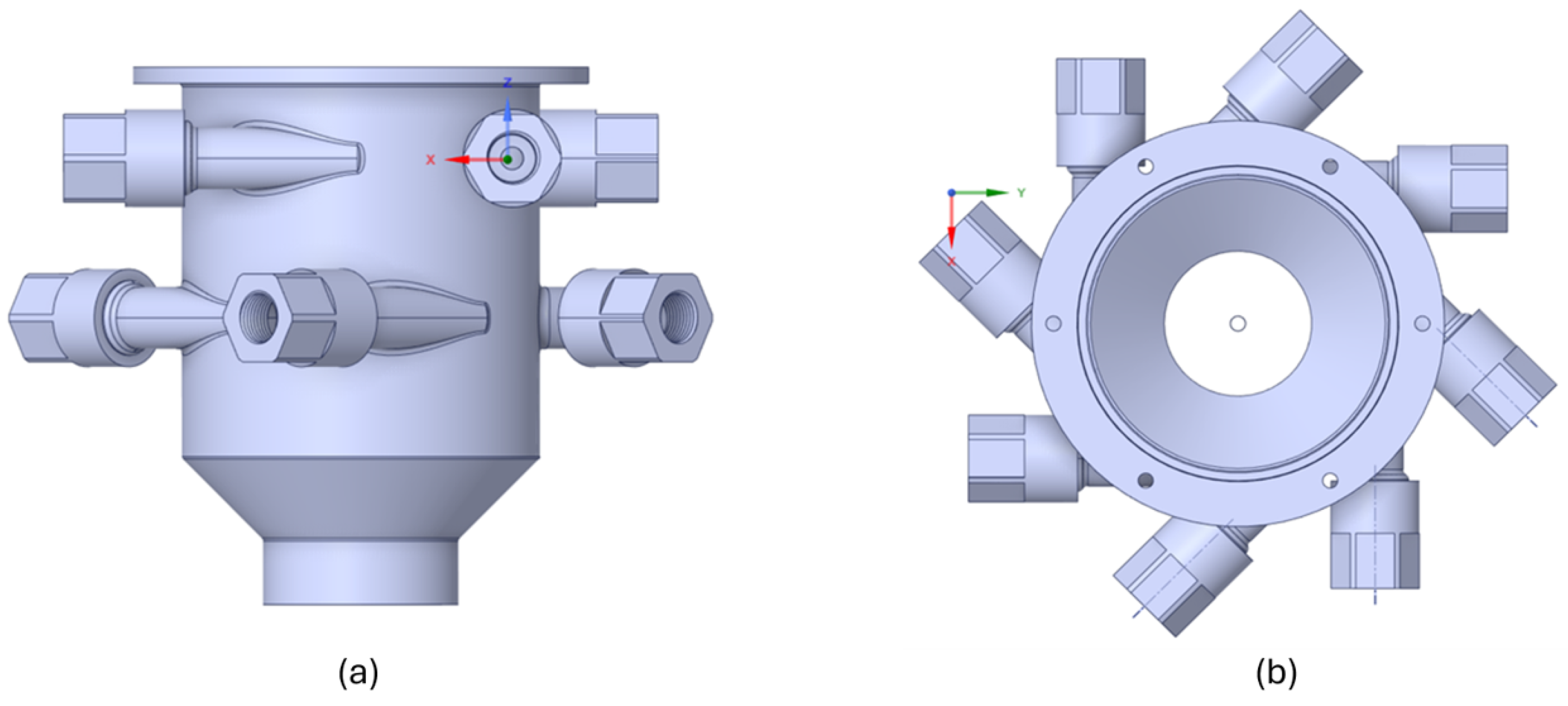
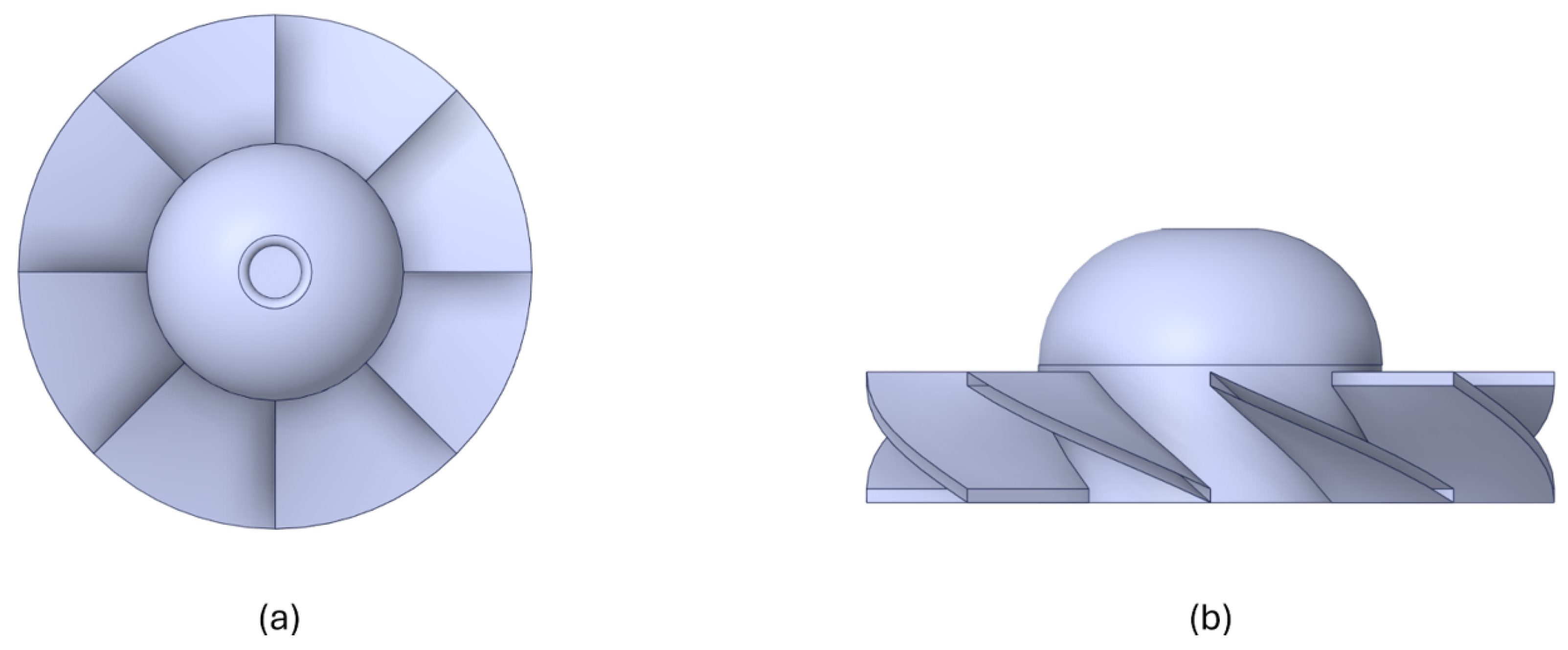
In a general overview, the geometry of atomizers encompasses various designs, each influencing spray characteristics and fluid dynamics. Two configurations (among many) are shown in Figure 1: (a) conical pressure-swirl atomizers, which operate with a higher flow rate, promoting a steady liquid discharge and uniform distribution, and (b) tangential pressure-swirl atomizers, whose design features multiple inlet channels arranged around a swirl chamber, allowing the fluid to enter at an angle and induce rotational motion before exiting through the nozzle [3]. Focusing on the second type, tangential centrifugal atomizers generate a spray characterized by a conical pattern, depending on the design of the outlet orifice and the distribution of the inlet channels. The spray angle typically varies between and , influenced by the injection pressure and orifice diameter. The atomization quality is evaluated by the mean droplet size (Sauter Mean Diameter, SMD), which can range between and , depending on the viscosity of the fluid and the tangential velocity imparted in the turbulence chamber [4].
Figure 1.
Illustration of the geometric parts and internal flow of the atomizer, (a) conical pressure swirl atomizer and (b) tangential pressure swirl atomizer.
In this study, these tangential centrifugal atomizers will be specifically employed as potential hydraulic turbines, leveraging their vortex generation and fluid acceleration properties to explore novel energy conversion mechanisms. This research aims to evaluate their feasibility in hydro-energy applications.
Figure 2 illustrates the geometric components and internal flow of the atomizer, providing a visual representation of how the fluid enters, circulates through the swirl chamber, and exits as a spray. The internal design, including the number and orientation of the inlet channels, directly influences the resulting spray pattern and droplet distribution. Additionally, factors such as chamber diameter, nozzle shape, and injection pressure play a crucial role in determining the stability and dispersion characteristics of the atomized fluid.

Figure 2.
Illustration of the geometric parts and internal flow of the atomizer.
Convetionally, the study of particle size and spray angle are particularly important since they are delimited by their application environment. For example, a higher-pressure rate will generate smaller droplets and a larger spray angle [5]. On the other hand, the mean Sauter diameter increases due to the coalescence of large droplets moving under the atomizer [6]. In this sense, recent contributions in this area were developed using image processing algorithms [7] to predict SCA, without the need to acquire sophisticated equipment such as PIV.
A way to classify atomizers is according to the dimensions of their outlet orifice, more specifically by the aperture coefficient parameter C, which relates the radius of the swirl chamber and the radius of the atomizer outlet. Based on this parameter, open C=1 and closed C>1 atomizers are obtained (Figure 3).
Figure 3.
Geometric configuration of atomizers according to C.
It was shown that an atomizer with an open end consumes a greater mass flow, compared to a closed one with the same number of channels “n” [8]. Likewise, in [9] it was revealed that it is important to control the mass flow that enters the atomizer, since it directly impacts the thickness of the liquid film. It is important to highlight that [8] is taken as background for this research, because it is vital to increase the thickness of the liquid film to ensure that the blades of the proposed internal rotor impact the injected fluid. Ultimately, this study will start from the design equations of centrifugal atomizers, where the proposed model will be validated using numerical simulations in Ansys Fluent.
2. Mathematical Models
2.1. Mathematical Model of the Atomizer Without Considering Losses
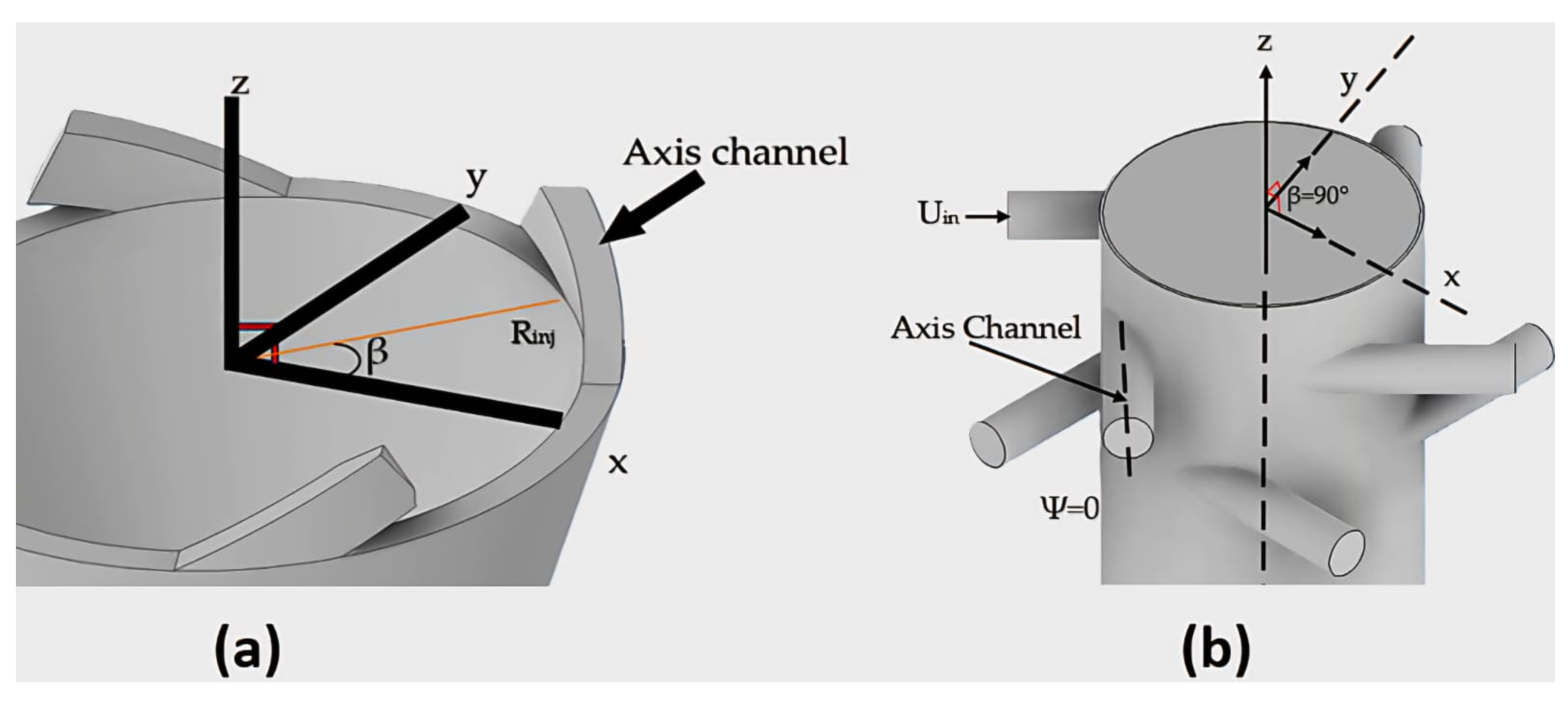
The mathematical model used for the design of the atomizer was the one developed by Rivas [10], as it is directly related to the dimensions of the swirl chamber. This model offers the possibility of obtaining the geometric characteristics of a type of atomizer, varying the angles of incidence of the inlet channels: and . For example, in the case of a tangential type: and . This mathematical model is based on what was proposed by Abramovich [11] using an ideal type of approach, without considering losses, and Kliachko [12] which considers fluid friction.
Starting from the concept of conservation of angular momentum:
By ordering the equations and applying the concept of continuity, we obtain, under steady state, the relationship of the tangential component of the velocity and the distance from the axis of the atomizer to the axis of the inlet channel (Equation (3)).
In the same way, it is possible to find the axial velocity of the liquid, using the continuity equation (Equation (4)). Consequently, the total velocity of the fluid in the injector can be calculated in the following way, neglecting its radial component (Equation (5)).
Another important parameter is the filling coefficient (Equation (6)), which relates the circular crown-shaped section of water formed in the swirl chamber (delimited by the radius of the air core ) in relation to the radius of the exit hole . Logically, indicates that the swirl chamber is filled with fluid, without the presence of the air core.
The discharge coefficient evaluates the actual mass flow (considering losses) in relation to the ideal mass flow. Likewise, based on the constructive geometric parameter A and the total velocity of the fluid , it can be obtained based on (Equation (7)).
The constructive geometric parameter or Abramovich number relates the tangential and axial speed within the injector. It is also obtained based on the dimensions of the radius of the exit hole, the radius of the inlet channels, and the distance from the center of the atomizer to the center of the inlet channel. Applying maximum flow theory to the discharge coefficient expression , parameter A is obtained based on the filling coefficient (Equation (8)).
Furthermore, based on Kessaev and Kupatenkov [13], the spray half-angle can be calculated, using the relationship of the tangential velocity and the magnitude of the total velocity. Finally, by integrating the angular momentum, (Equation (9)) is obtained.
2.2. Mathematical Model of the Atomizer Considering Losses
As the viscosity of the fluid is taken into consideration, the presence of the Blasius coefficient is observed, given by (). In turn, it is necessary to consider the losses due to the geometric contraction of the inlet channels using (Equation (10)) to determine the tilt angle and accordingly use Figure 4 [14].
Figure 4.
Obtaining the loss coefficient , due to the geometry of the inlet channel.
On the other hand, the loss coefficient due to the friction of the liquid on the walls of the inlet channels is a function of the Blasius coefficient and the geometric characteristics of the inlet channel (Equation (11)). In this way, it is possible to obtain the total loss coefficient using Equation (12).
Considering these hydraulic losses, the equivalent constructive geometric parameter can be obtained considering losses according to Kliachko [15] (Equation (13)).
2.3. Hydraulic Head
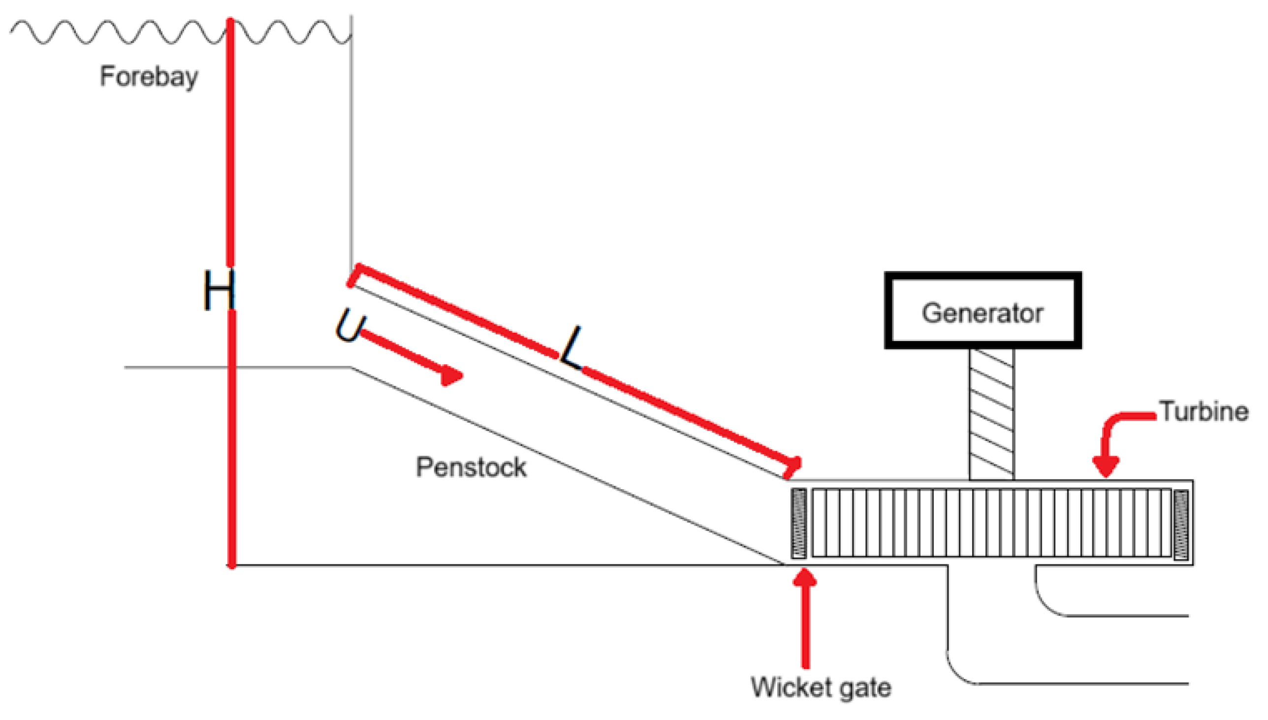
In hydroelectric power plants, the net head (H) is expressed as the difference between the stored head and the height of the fluid leaving the turbine [16,17], as it is presented in Figure 5. This parameter is vital for calculating the energy available in a tributary for the generation of electric power.

Figure 5.
Simple schematic of a hydroelectric plant.
2.4. Mechanical Power and Efficiency
It represents the useful work to move an object; in this case, the fluid hits the blades of the internal rotor, producing movement on the axis (Equation (16)). To calculate the efficiency of the system, the relationship between the useful mechanical power generated in the turbine shaft and the hydraulic power available in the water flow that feeds it is considered.
In the case of pressure-swirl atomizers, the equations directly relate to the injection pressure in the inlet channels. Therefore, it is possible to express the available hydraulic power through the equation shown in Equation (17).
3. Proposed Model
3.1. Swirl Chamber Structure
Table 1 shows the initial parameters for the design of the swirl chamber; the value of the mass flow was considered at 3.5 kg/s. Also, Table 2 shows the geometric parameters obtained from the conventional mathematical model based on the operating conditions of the atomizer.

Table 1.
Operation parameters of pressure swirl atomizer.
Table 2.
Pressure swirl atomizer dimensions calculated.
To obtain the second level of feed flow, the same dimensions of the atomizer are used at a single level, except for taking four input channels interspersed and giving them a vertical distance of 50 mm (Figure 6). Ref. [18] demonstrated that the height of the swirl chamber affects the atomization process, including the mass flow. In real applications, the selection of the atomizer manufacturing material must take into account surface roughness. Increased roughness can increase pressure losses, alter flow and spray angle, and affect droplet size distribution. It can also promote deposit buildup and wear. Therefore, it is crucial to choose materials and techniques that minimize these effects to ensure efficient atomization [19,20].

Figure 6.
Swirl chamber housing. (a) Front view of the dual-level scale atomizer and (b) plan view of the atomizer on a double-level scale.
3.2. Stabilizer
The purpose of this research is to implement an internal rotor, so it is necessary to prevent the rotor from suffering axial interferences that could reduce the performance of the proposed system. As can be seen in Figure 7a,b, the profile of the blades is closed, with a total of 8; the upper area is cylindrical with roundings to facilitate the discharge of water through the outlet orifice. It is necessary to clarify that it is proposed to design the structure of the atomizer with the stabilizer included so that it forms part of the casing of the turbulence chamber.
Figure 7.
Lower stabilizer design. (a) Plan view and (b) front view of the stabilizer designed in Spaceclaim.
3.3. Internal Rotor
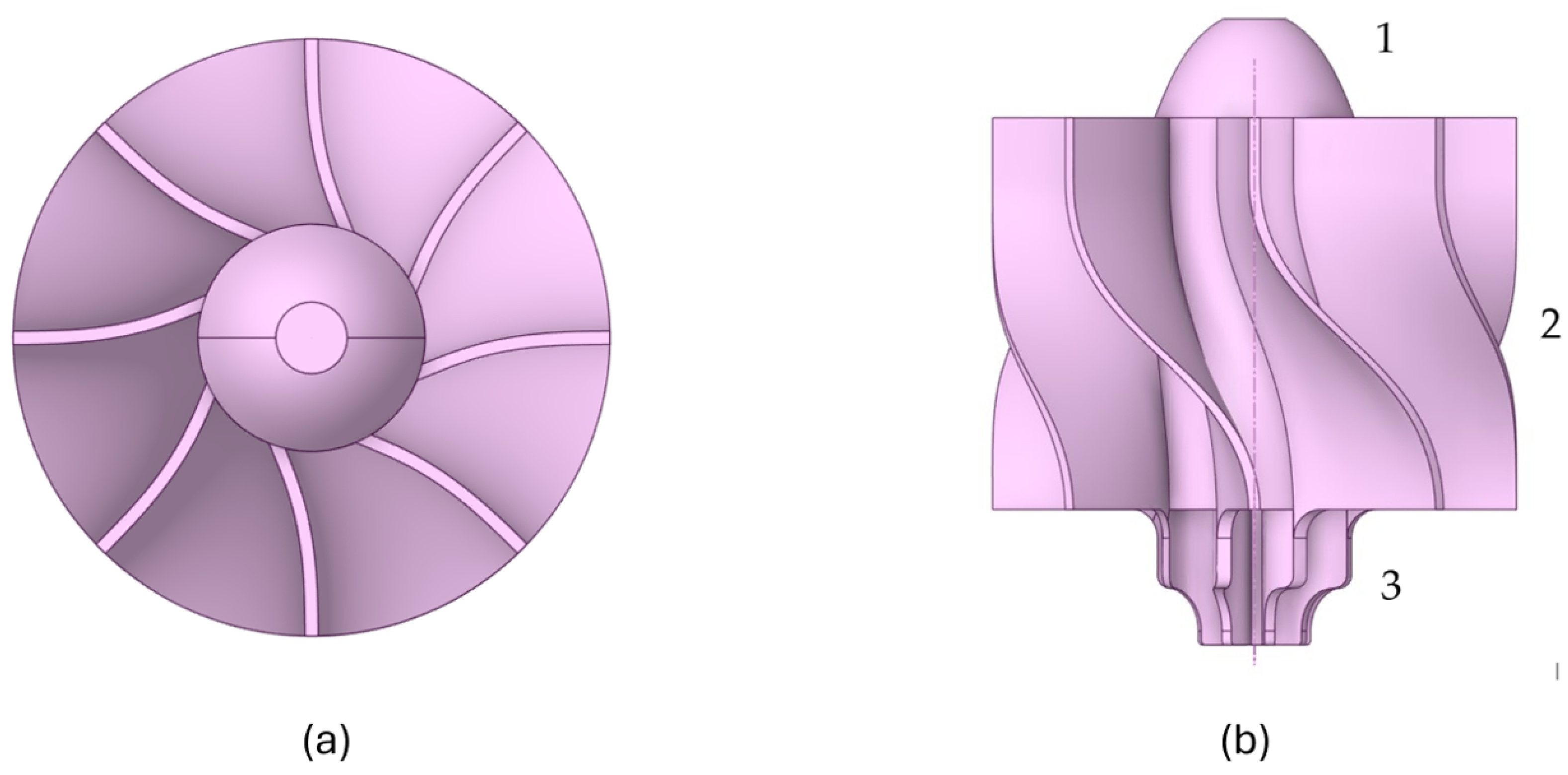
The rotor design in Figure 8a,b has a diameter of 96 mm and a height of 110 mm. The objective is for the main blades to hit the fluid closest to the inner face of the swirl chamber, the area where the water speed is highest in this type of atomizers [18]. Also, the design considered the vortex-type flow distribution generated within the atomizer. Therefore, its geometry considers three distinctive factors: dome, spiral-type blades, and a pre-stabilizer.
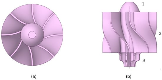
Figure 8.
Internal rotor design. (a) Plan view and (b) front view (1—dome, 2—blades, 3—pre-stabilizer) designed in Spaceclaim.
- The dome allows the portion of water formed in the upper area of the atomizer to be distributed more efficiently towards the main blades.
- Spiral-type blades allow for the centrifugal fluid movement to not be abruptly interrupted and for turbulence not to form at the intersections [21].
- The pre-stabilizer serves to redirect the portion of air that filters through the outlet hole, redirecting the fluid towards the walls of the swirl chamber and expelling it through the lower area.
The proper selection of materials for turbine components, such as the internal rotor and the stabilizer, is crucial to ensuring optimal performance and long service life. Below is an evaluation of potential materials, highlighting their key properties (Table 3).
Table 3.
Material properties comparison.
Stainless steel 316 was selected to perform the simulations of the turbine components, facilitating structural analysis. This material has a tensile strength of 580 MPa, a Young’s modulus of 290 GPa, and a density of 8.027 g/cm3, allowing for a more accurate evaluation of its behavior under operating conditions.
Compared to other materials such as aluminum 6061 (290 MPa, 69 GPa), PLA (52 MPa, 4.1 GPa), and ABS (50 MPa, 2.5 GPa), stainless steel 316 provides more precise results in terms of stress and deformation. Although titanium Ti-6Al-4V (895 MPa, 113 GPa) exhibits superior mechanical properties, stainless steel 316 was chosen due to its extensive use in computational studies and its compatibility with simulation tools, enabling a more detailed structural performance analysis.
4. Results
4.1. Mesh Conditions
Once the system is assembled with all the subparts, Figure 9 is obtained, where the volume of fluid to be used for the simulations can be seen.
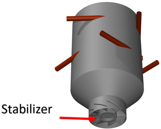
Figure 9.
Internal flow volume extract considering atomizer, stabilizer, and internal rotor.
Recent studies on atomizers have employed the technique to guarantee the accuracy of their models, ensuring proper resolution of the boundary layer. In this research, the same methodology is adopted due to its advantages, such as improved prediction of flow behavior near walls, which allows for more accurate results in the simulation of momentum and energy transfer phenomena [22,23]. Unlike the grid convergence index (GCI) method, which primarily assesses numerical convergence through successive mesh refinements, provides a physically meaningful criterion that ensures proper near-wall resolution and the accurate capture of wall shear stress and turbulence effects near solid boundaries.
Previous research has shown that wall shear stress and drag coefficient estimations are highly sensitive to variations in , even when values remain within the viscous sublayer [24]. Given the importance of correctly resolving these forces in the atomizer design, maintaining within the appropriate range ensures that turbulence interactions with the wall are properly captured, reinforcing the validity of the selected approach.
The dimensionless wall distance is a critical parameter in computational fluid dynamics (CFD) that quantifies the relative position of the first computational cell near a solid boundary. It is used to assess whether the mesh resolution is sufficient for accurately capturing the boundary layer effects, especially in turbulent flows. The equation governing is shown in Equation (18).
This parameter is particularly crucial in high-accuracy CFD simulations where near-wall turbulence needs to be resolved rather than modeled. In simulations using turbulence models such as SST k-, a fine mesh is required near the walls, ensuring that remains below 5 [25]. If is too high, the solver will fail to capture the viscous sublayer, leading to inaccurate estimations of wall shear stress, velocity profiles, and flow separation. The shear velocity Equation (19) is a fundamental quantity that represents the velocity scale associated with turbulent shear stresses near the wall. Also, wall shear stress , which results from the interaction of the fluid with the solid surface and determines the forces exerted by the fluid on the wall (Equation (20)). Finally, the skin friction coefficient can be estimated for turbulent boundary layers using
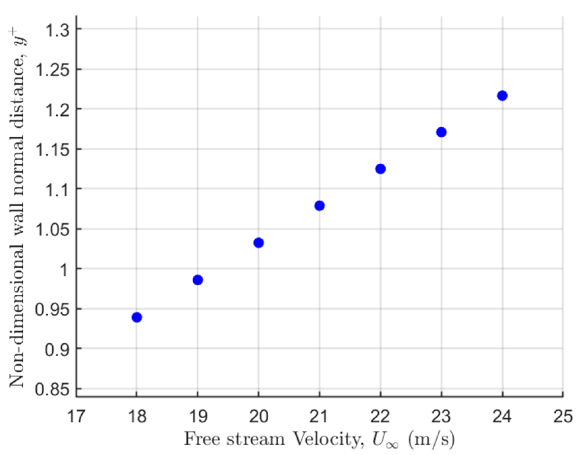
To determine the range of values in the simulation, an inlet hydraulic diameter mm of and a free-stream velocity between 18 m/s and 24 m/s are considered. By applying Equation (21), the friction coefficient is found to be within the range of [0.005202883; 0.005464308].
Using the obtained values and applying Equations (19) and (20) to determine the wall shear stress and friction velocity, respectively, the parameter is calculated considering the minimum cell distance to the wall, set at mm. By solving Equation (18), the resulting values are found to be within the range of 0.939–1.216 (Figure 10).
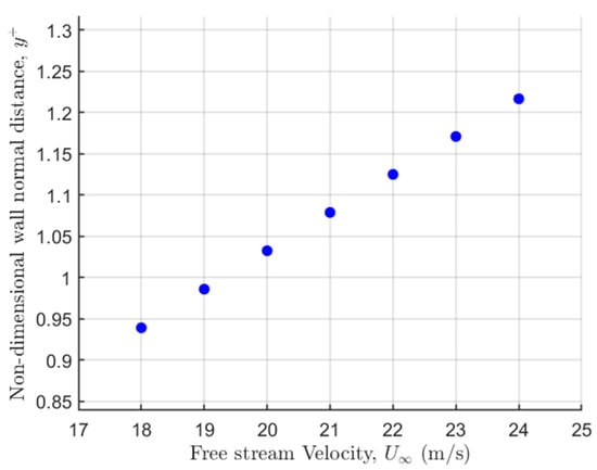
Figure 10.
Front view of mesh generation of double manifold atomizer with stabilizer and rotor included.
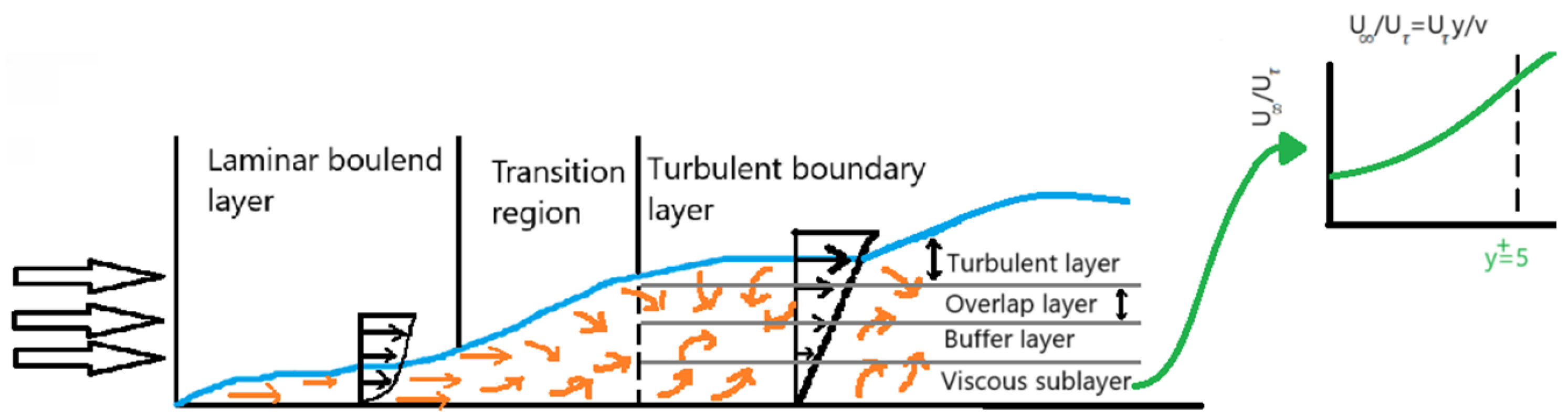
Figure 11 shows that the obtained values fall within the viscous sublayer region ( < 5), indicating that the standard wall function can be applied in turbulence models such as SST [25]. Finally, Figure 12 shows the refinement in the channel inlet applying this meshing technique.
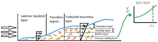
Figure 11.
Law of the wall.
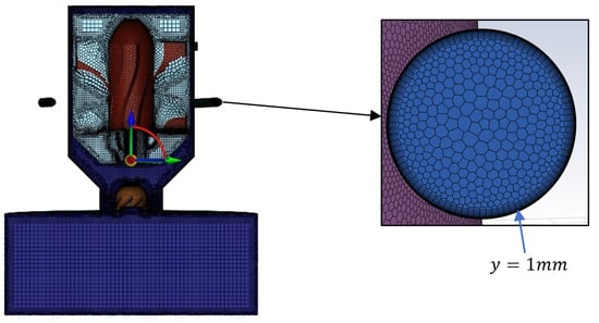
Figure 12.
Front view of mesh generation of double manifold atomizer with stabilizer and rotor included using O-Grid technique.
Table 4 shows mesh characteristics in all six cases considered, the first three supplying fluid under nominal conditions (i.e., 350 kPa, feeding flow in both manifolds, only in the lower manifold and the upper manifold), to quantify the turbine performance: torque, angular velocity, and efficiency. Additionally, in the other three cases, a flow supply in both manifolds was considered for the following pressures: 250 kPa, 300 kPa, and 400 kPa, in order to evaluate the hydraulic consumption of the system.
Table 4.
Cases and characteristics of poly-hexcore meshes.
4.2. Boundary Conditions
The computational domain was defined under Cell Zone Conditions as a mixture, ensuring a proper multiphase interaction. To facilitate fluid exchange between the internal rotating domain (rotor) and the stationary domain, an interface was created to maintain numerical consistency across the transition. Boundary conditions were specified as follows: for pressure inlets, the Direction Specification Method was set to Normal to Boundary, ensuring an accurate inflow direction, while for outlets, the Backflow Direction Specification Method was set to From Neighboring Cell, allowing for a realistic backflow behavior in recirculations produced by the air core. Despite being part of the rotating domain, the internal rotor was defined as a stationary wall with a no-slip condition to prevent conflicts with the dynamic mesh configuration, ensuring stable numerical behavior and accurate force transfer within the simulation. Table 5 shows the configuration of inlets and outlets considered for the simulation of all six analyzed cases.
Table 5.
Boundary conditions setting.
To simulate the mechanical power generated by the rotor in a real scenario, input parameters such as the multiphase VOF model and a surface tension coefficient of 0.073 were considered. The SST k- turbulence model was chosen because it is widely used for hydraulic turbine applications [26,27] due to its ability to accurately capture near-wall flow phenomena, such as boundary layer separation, and realistically represent pressure gradients and vortex formation. This was demonstrated in gravitational water vortex hydraulic turbines [28], where a good numerical correlation with experimentally generated vortex profiles was achieved. Moreover, it has been observed that this model provides a strong agreement with measured torque data in turbomachinery [29] and can also accurately predict jet dissipation and air–particle interactions, phenomena directly applicable to atomizers [30]. To complement this analysis, simulations were also performed using the k- turbulence model exclusively to evaluate its impact on power prediction. This model, often employed in hydraulic applications, is particularly useful for estimating large-scale flow structures and energy dissipation [31], which directly influence torque and rotational speed calculations. The comparative study between both turbulence models is essential to assess their accuracy in predicting the dynamic response of the rotor. Given that mechanical power output is derived from the product of torque and angular velocity, discrepancies between the models can indicate variations in the predicted energy transfer efficiency. To enable rotation, six degrees of freedom (6-DOF) for rigid bodies were activated, allowing for rotation around the Z-axis. The rotor’s mass and moment of inertia () were calculated using SolidWorks version 2024 with stainless steel 316 material properties. Reports on tangential velocity, moment, and angular velocity were generated.
4.3. Supplying Flow from Both Manifolds, Lower Manifold, and Upper Manifold
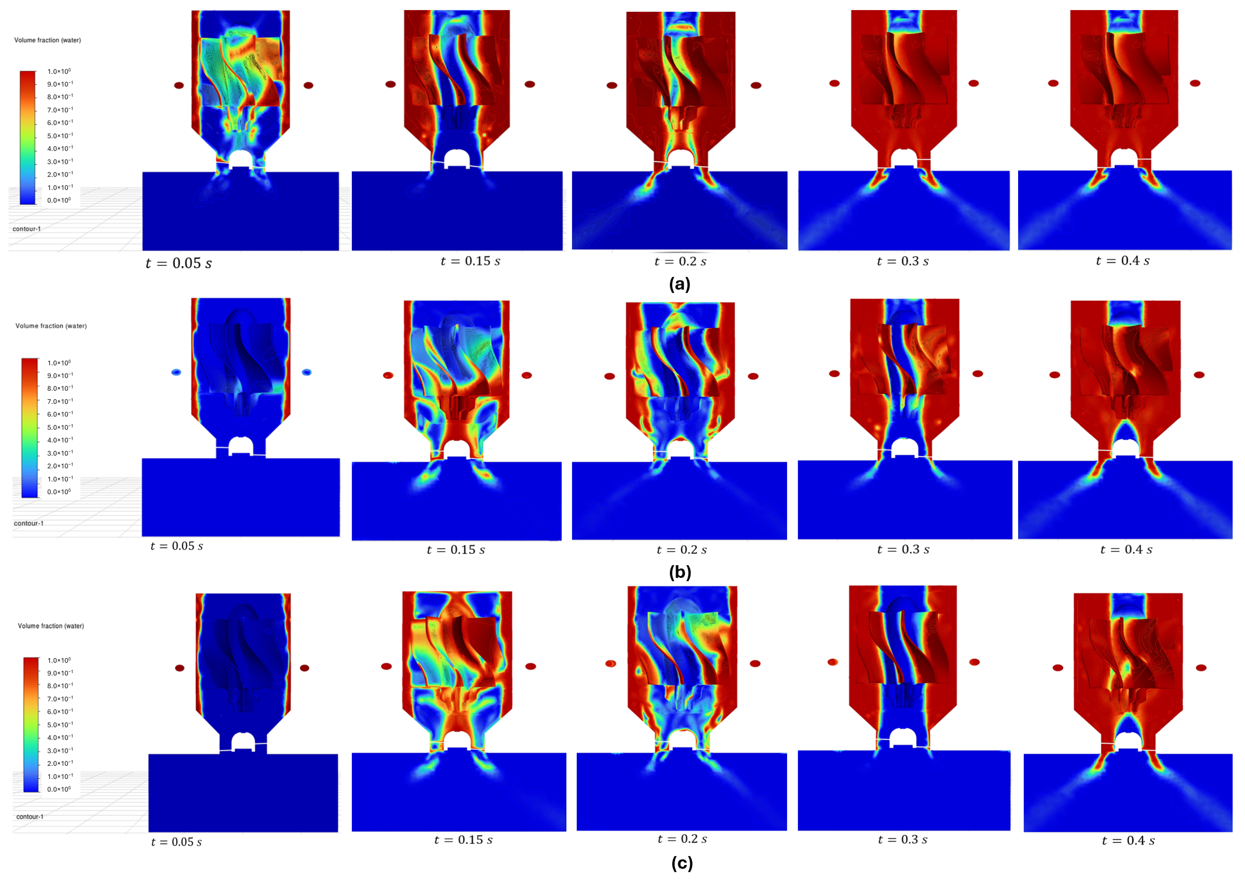
Below are the captures of the internal flow at the simulation instants: 0.05, 0.15, 0.2, 0.3, and 0.4 s. Figure 13a shows the atomizer fed by the eight channel inlets in nominal conditions ( kPa) with the rotor included. In the first captured instant (0.05 s), it is observed that a small portion of the liquid inside the swirl chamber hits the lower area of the blades and impacts the pre-stabilizer. In turn, starting at instant 0.15 s, it is observed that the liquid film formed gains greater thickness, and the portion of the fluid that collides with the blades is more uniform. Also, it is shown that, at 0.2 s of the simulation, a portion of the air enters through the stabilizer of the outlet orifice, directly affecting the pre-stabilizer of the internal rotor. This small interference is canceled moments later at 0.3 s and 0.4 s, where a quasi-stationary equilibrium is reached, resulting in a spray pattern with certain deformations and a small portion of air lodged in the upper area of the atomizer, surrounding the internal rotor dome.
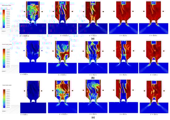
Figure 13.
Capture of the transient regime towards the quasi-stationary equilibrium at the simulation instants: 0.05, 0.15, 0.2, 0.3, and 0.4 s, supplying flow for both manifolds (a), lower manifold (b), and upper manifold (c).
Figure 13b,c show the results for the same supply pressure as the previous case but injecting only into the lower and upper manifold, respectively. In the first moments, significant differences are shown in the development of the internal flow. For example, in Figure 13b at moment 0.15 s, it is seen that the lower area of the internal blade is substantially covered by water because it is the direct entry area of the fluid. Likewise, at that same simulation moment, Figure 13c shows that a large part of the surface of the internal rotor is covered with water due to the path it makes from the upper area of the inlet to the orifice outlet.
For both cases, at instant 0.4 s, it is seen that the spray pattern is a little more uniform, keeping small differences with respect to the previous case. In turn, the formation of a tetrahedral-shaped air zone above the stabilizer due to the air core can be highlighted. Similarly, it is highlighted that the quasi-stationary equilibrium is reached later compared to case (a). As expected, this is due to the intake flow into the system (which will be discussed later in the power results obtained), which also leads to changes in the internal flow obtained in quasi-stationary equilibrium.
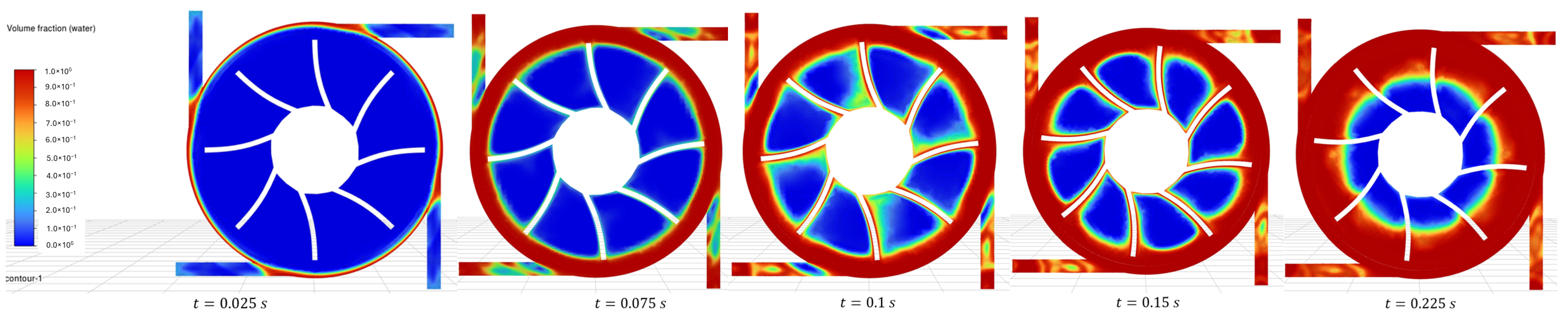
It is also important to highlight that, for cases (b) and (c) which have inlet channels without water entry, a counterflow is formed due to oversaturation of the swirl chamber, as the numerically obtained flow rate exceeds the design value of 3.5 kg/s (demonstrated in Section 4.4), leading to localized pressure gradients that force water and air portions to enter these unused inlet channels in the first simulation instants, as shown in Figure 14, causing portions of water with air particles entering and being seen as a hydraulic loss, since they do not contribute to the movement of the internal rotor.
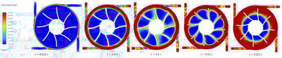
Figure 14.
Internal flow of inlet channels without hydraulic supply at simulation instants: 0.025, 0.075, 0.1, 0.15, and 0.225 s.
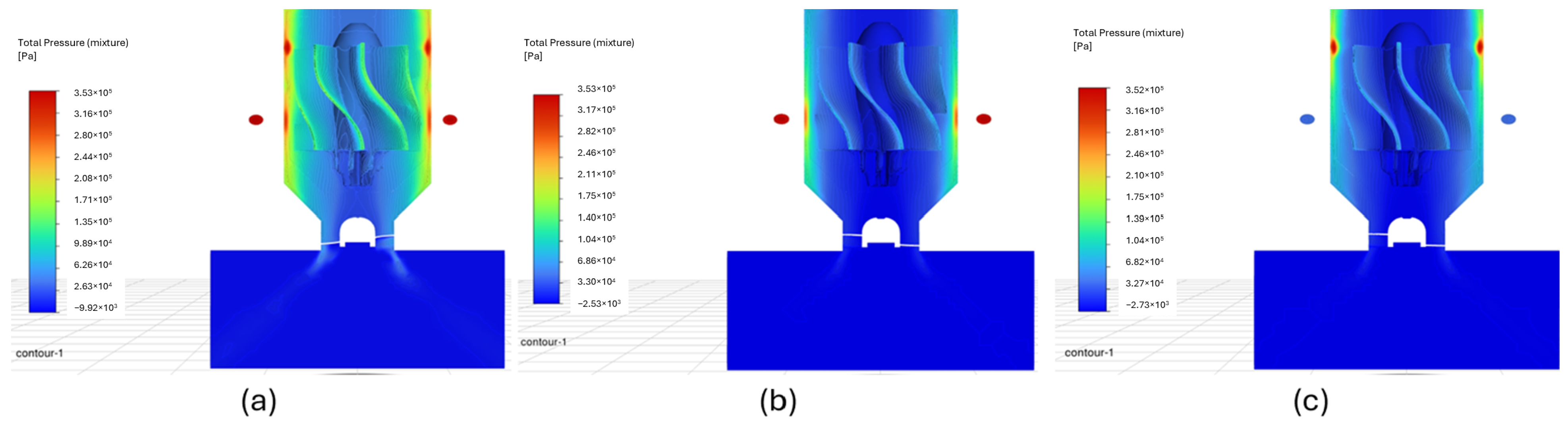
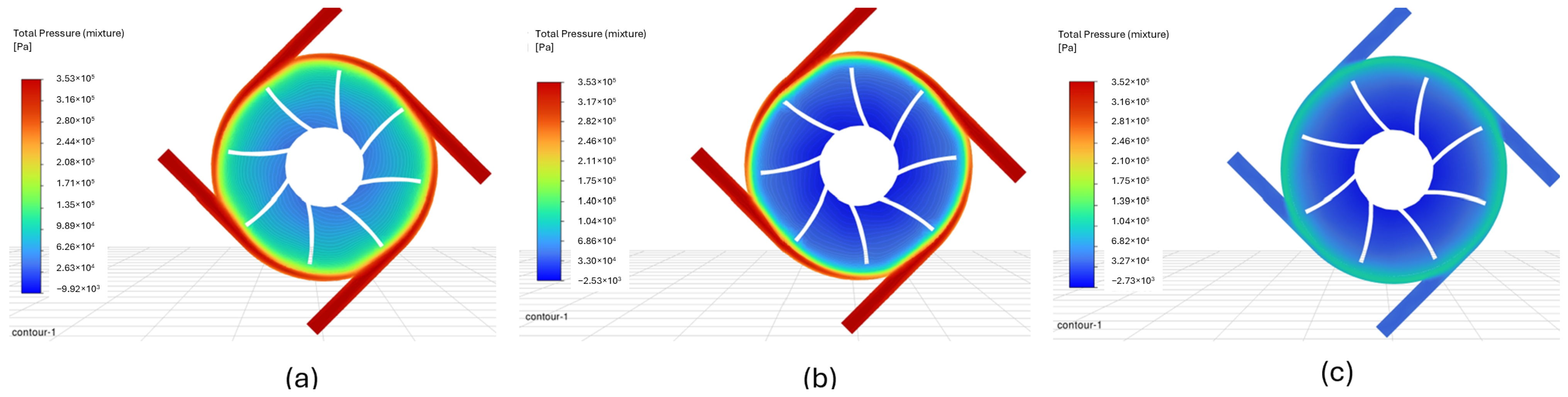
Also, in Figure 15 (in a, b, and c) high-pressure regions (depicted in red) are located near the inlets, where the fluid enters the swirl chamber with significant energy. As the fluid progresses through the system, the pressure decreases (shifting to blue), particularly in the center and downstream of the chamber, indicating the expansion effect of the fluid causes a decrease in pressure, since the pressure energy is redistributed to adapt to the increase in volume and, in part, is converted into kinetic energy that will cause the turbine’s movement.
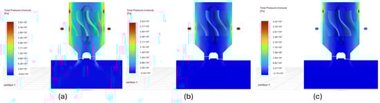
Figure 15.
Front view of the total pressure distribution of the fluid mixture within the swirl chamber, supplying flow at 350 kPa from both manifolds (a), lower manifold (b), and upper manifold (c).
Figure 15a shows that the pressure distribution is more uniform from the exit of the fluid from the channel inlets to the surfaces of the internal rotor, observing that the fluid enters with 350 kPa of pressure (adopting reddish colors) and when approaching the walls of the swirl chamber decays to approximately 300 kPa, to finally impact the internal rotor blades with a pressure of 124 kPa. This is unlike Figure 15b,c, where it is observed that the fluid transitions abruptly up to 80 kPa in the areas closest to the internal rotor blades.
This phenomenon can be attributed to the sudden expansion of the fluid as it fully traverses the inlet channels. In a quasi-steady state, the fluid inundates the swirl chamber, causing it to become fully saturated. As the water travels vertically within the atomizer’s internal structure, attempting to fill the chamber, it experiences significant energy losses due to the combined effects of gravitational forces, increased turbulence, and friction against the chamber walls. This contrasts with case (a), where the activation of the second manifold offsets these losses by enhancing the dynamic pressure of the adjacent fluid.
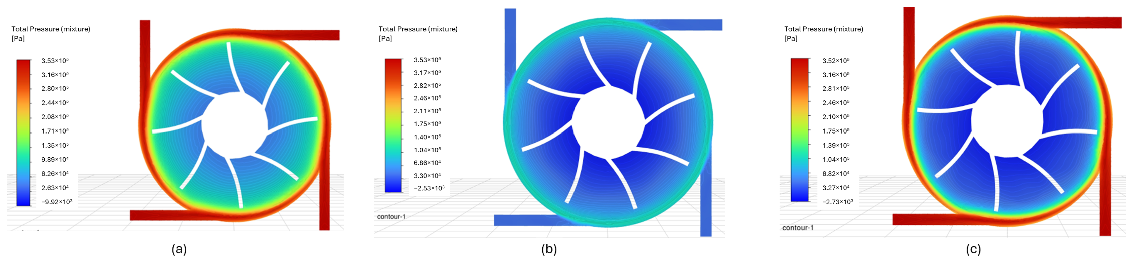
Figure 16a shows what was previously explained, highlighting that the zone of lowest pressure (referring to the central zone of the atomizer) is around 51.7 kPa, a product of the collision of the particles with the blades of the internal rotor, causing considerable load losses in that area. On the other hand, Figure 16b illustrates the abrupt pressure change resulting from the fluid’s transition from the lower to the upper manifold. Significantly low pressures, approximately 50.7 kPa, are observed in the inlet channel zones without supply, a consequence of the counterflow described earlier. Additionally, in Figure 16c, the pressure contours within the swirl chamber are noteworthy, ranging from 277 to 256 kPa. The central surface of the atomizer, in contrast, exhibits a pressure of 14.99 kPa.
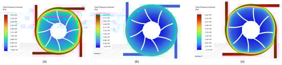
Figure 16.
Cross-sectional view of total pressure distribution of the fluid mixture within the swirl chamber from the upper manifold, supplying flow at 350 kPa from both manifolds (a), lower manifold (b), and upper manifold (c).
The pressure contours in Figure 17a reveal a pattern that is almost identical to the one previously analyzed, as exemplified by Figure 16a. Meanwhile, the most notable feature in Figure 17b is the pressure observed in the central area of the atomizer surrounding the rotor dome, which measures approximately 15.2 kPa. This value is slightly lower than the 18.5 kPa observed in Figure 16c, despite the fluid being injected through different manifolds in the atomizer. This similarity suggests that cases (b) and (c) are practically analogous in terms of pressure distribution. A comparable observation applies to Figure 17c and Figure 16b, as the minimum and maximum pressure values are nearly identical, regardless of the manifold used for fluid injection in each case.
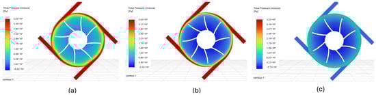
Figure 17.
Cross-sectional view of total pressure distribution of the fluid mixture within the swirl chamber from the lower manifold, supplying flow at 350 kPa from both manifolds (a), lower manifold (b), and upper manifold (c).
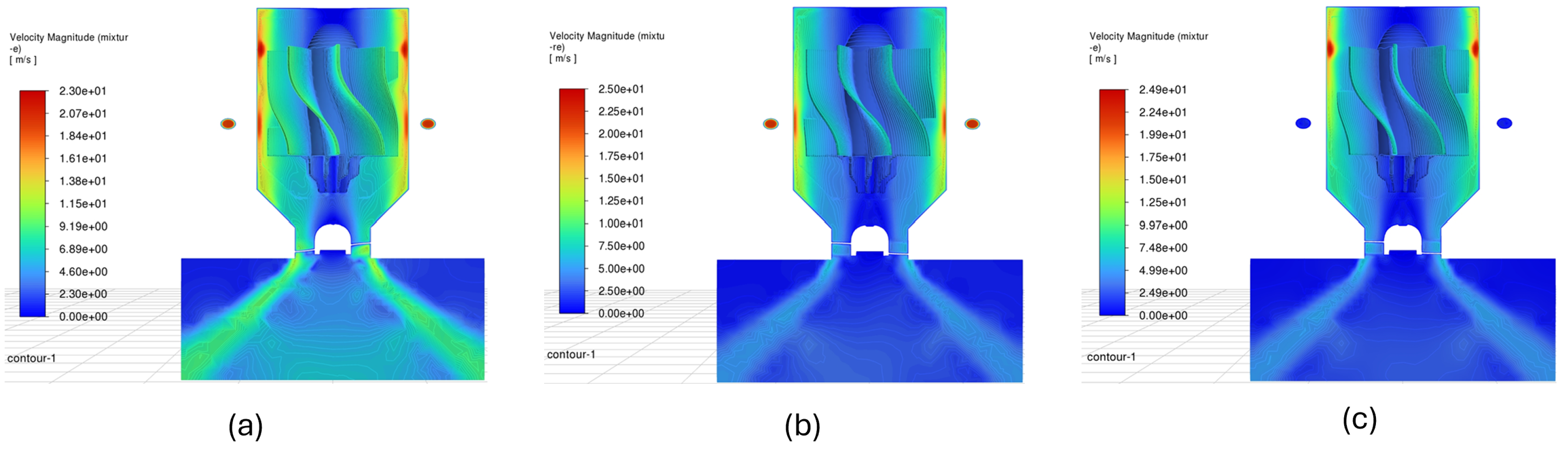
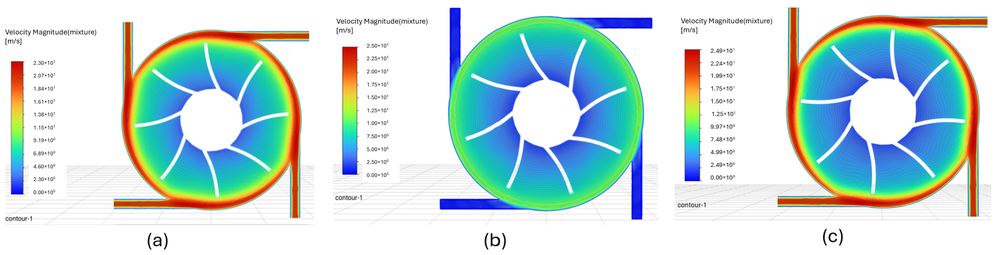
Figure 18a shows that, as occurs with the pressures, the velocity profile in the atomizer exhibits a more uniform distribution than the other cases analyzed. Additionally, the spray outlet adopts a more intense color, reaching 11.2 m/s. This is logically caused by the greater mass flow that passes through the eight channel inlets. Likewise, it is important to highlight that the particles with considerable speed are found in the external area of the blades, overlaid with green.
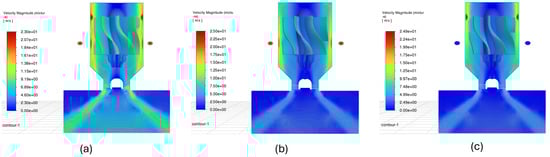
Figure 18.
Front view of velocity magnitude of the fluid mixture within the swirl chamber, supplying flow at 350 kPa from both manifolds (a), lower manifold (b), and upper manifold (c).
Figure 18b,c show that the atomizer’s exit velocities achieved were quite close: 6.5 m/s and 6.98 m/s, respectively. The same occurs for the fluid found in the lower area of the internal rotor, where the backflow produced by the air core occurs, since for both cases values of 0.75 m/s were recorded.
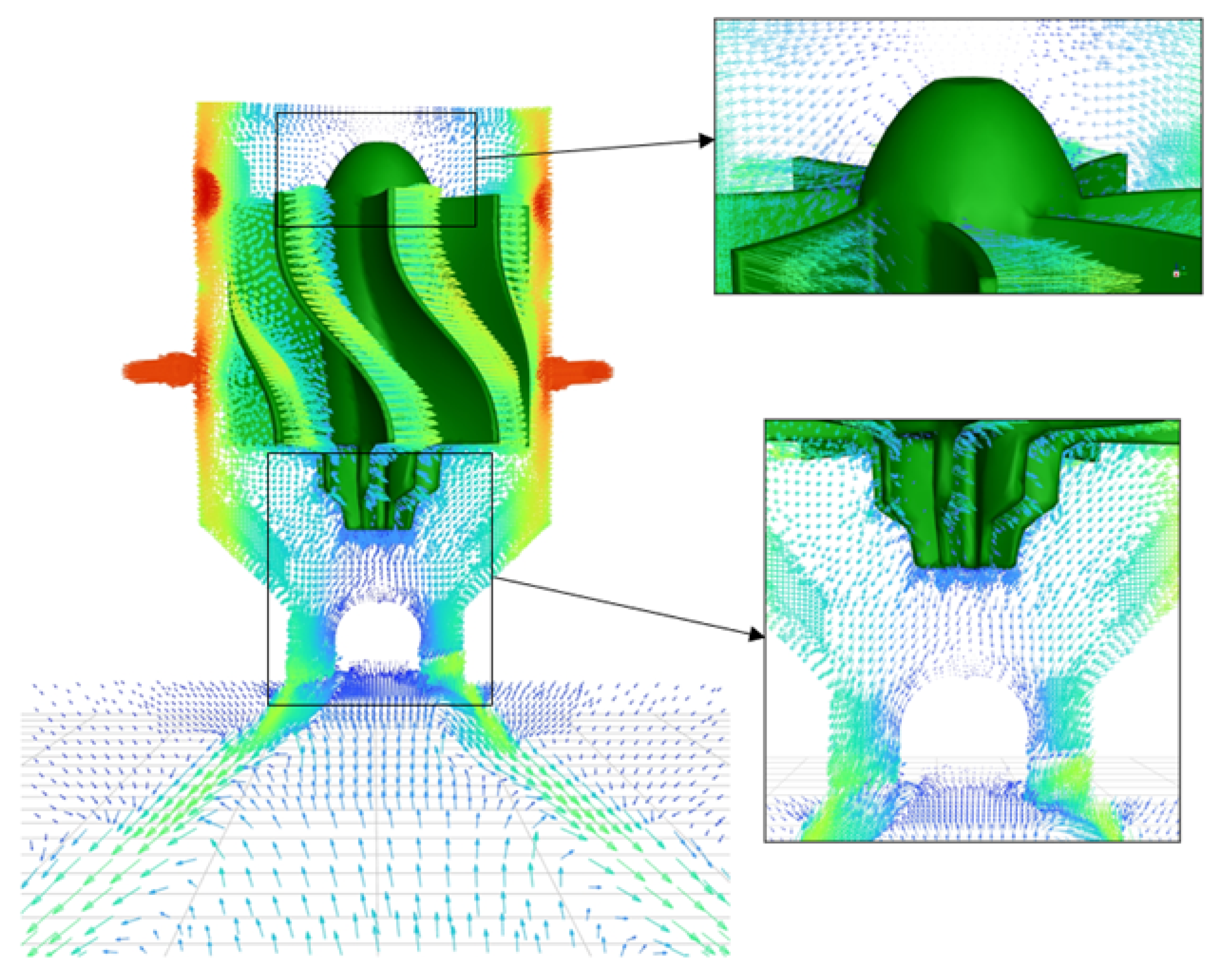
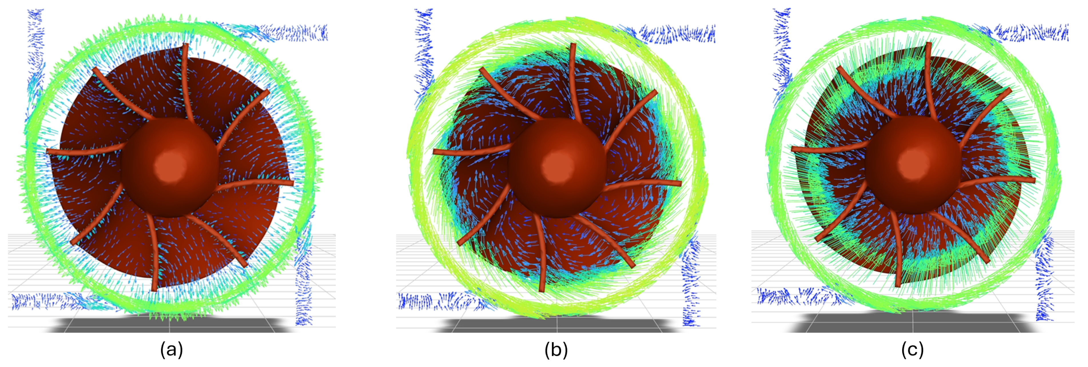
For the three cases, it is agreed that the lowest speeds are found in the upper area of the internal rotor, where the dome is located (0.24 m/s). In that sense, the behavior of the internal flow is shown in Figure 19, which illustrates how the upper dome helps direct the fluid towards the blades, ensuring uniform distribution and minimizing unwanted turbulence.
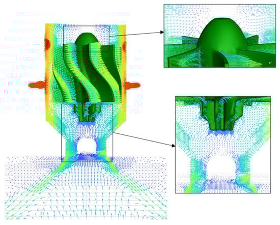
Figure 19.
Front view of velocity vector of the fluid mixture within the swirl chamber, supplying flow at 350 kPa from both manifolds.
Likewise, the performance of the stabilizer is observed. As expected, part of the air remains attached to its structure, preventing this fluid from entering the swirl chamber. However, a small portion in the central area manages to penetrate the structure. This behavior is noticeably visible in the lower part of the atomizer, but as the air approaches the central areas of the swirl chamber, this ascending velocity profile is considerably attenuated and redirected by the pre-stabilizer at the base of the internal rotor.
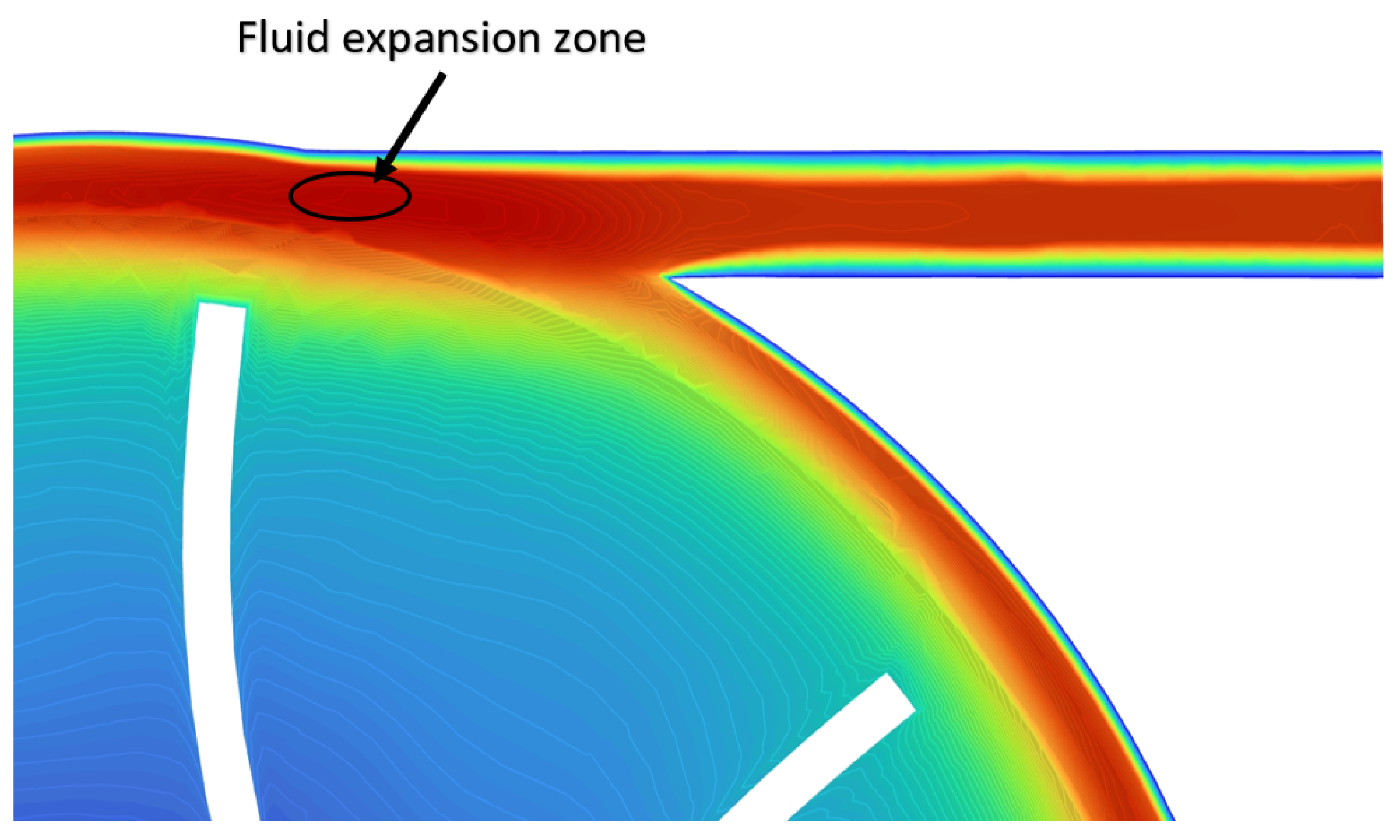
As already mentioned, the walls of the atomizer are those that have the highest velocity particles in the system, but it is important to highlight that this behavior is substantially predominant in the fluid expansion zones. As can be seen in Figure 20, the maximum velocities found for all cases are located immediately after the fluid has completely crossed the inlet channel. From there, it is highlighted that the intense orange profile gradually fades slightly after traveling along the walls of the swirl chamber and hitting the turbine blades.

Figure 20.
Fluid expansion zone where the maximum velocity obtained is found.
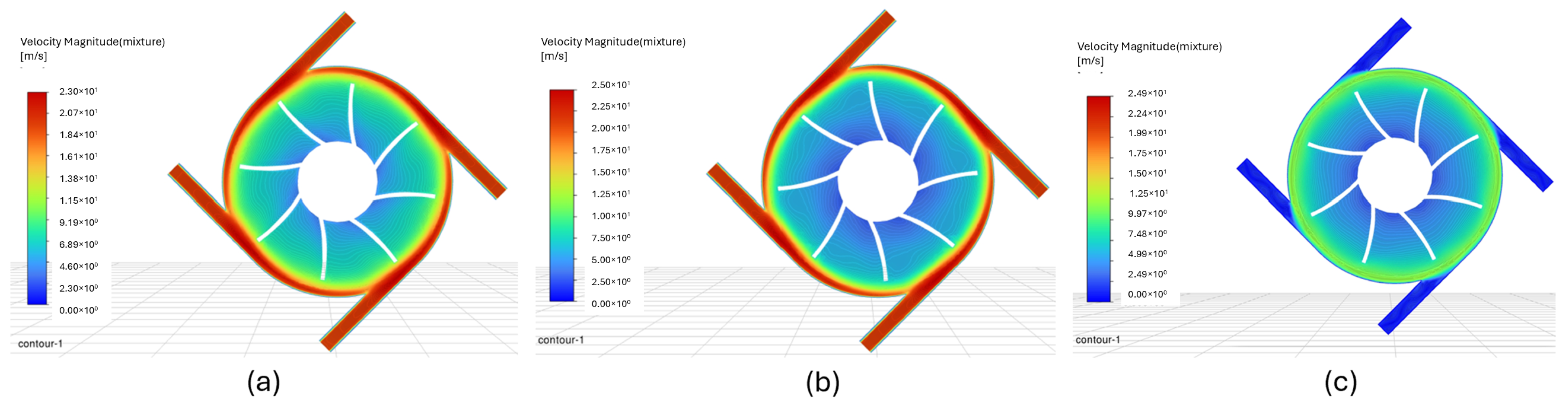
In Figure 21a, the fluid stored in the inlet channels, highlighted in orange, exhibits velocities ranging from 19.8 m/s to 23 m/s within the fluid expansion zone. The latter value is the lowest among the maximum values reached in all three cases analyzed. This behavior can be explained by the previously analyzed pressure distribution: as the pressure drop is abrupt, the velocity increases following the pressure gradient. Additionally, the low-pressure regions create a suction effect, drawing more fluid into these areas and further accelerating the flow.
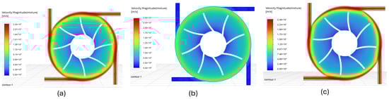
Figure 21.
Cross-sectional view of velocity magnitude of the fluid mixture within the swirl chamber from the upper manifold, supplying flow at 350 kPa from both manifolds (a), lower manifold (b), and upper manifold (c).
Evidence of this is seen in the pressures recorded in the central area of the atomizer (50.7, 15.2, and 18.5 kPa for cases (a), (b), and (c), respectively), with case (a) demonstrating more controlled particle velocities without sudden variations. On the other hand, Figure 21b shows that the velocity along the contours of the swirl chamber is approximately 10.9 m/s, while in the central area of the atomizer it reaches 2.99 m/s. Notably, the portions of water stored in the inlet channels without supply exhibit significantly lower velocities, around 1.5 m/s. In Figure 21c, as expected, the most abrupt changes in particle velocity occur in the region surrounding the inner rotor, with bluish contours indicating values ranging from 7.7 m/s to 3.2 m/s (in the center of the chamber).
Figure 22a shows that the behavior of the fluid in the cross-section of the lower manifold is nearly identical to what is observed in Figure 21a, with no notable differences. Additionally, Figure 22b,c do not reveal significant changes in the velocity distribution of the water. However, in the third case, the counterflow occurs at a lower region, and the velocity adjacent to the chamber walls is 10.4 m/s (highlighted in green), which is similar to the value obtained in Figure 21b.
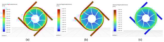
Figure 22.
Cross-sectional view of velocity magnitude of the fluid mixture within the swirl chamber from the lower manifold, supplying flow at 350 kPa from both manifolds (a), lower manifold (b), and upper manifold (c).
Figure 23 demonstrates the velocity profiles of the particles located at the entrances of the channels without hydraulic supply. It can be observed that the reflux entering these channels has practically negligible velocities, along with the formation of small vortices and recirculations. On the other hand, it is observed that, despite the unfavorable behavior of this portion of the liquid, a significant number of particles (colored in green) tend to generate the desired swirl effect to induce rotation. Finally, to mitigate backflow, the implementation of flexible silicone membranes as an anti-return system is proposed as a strategy. These membranes, located at the entrance of each channel (at the root of the swirl chamber walls), allow for the unidirectional passage of fluid and close automatically in the absence of supply, preventing the accumulation of liquid in the inactive conduits. Its compact design guarantees efficient sealing without altering the geometry of the system, nullifying the formation of vortices and improving the stability of the internal flow.
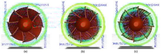
Figure 23.
Cross-sectional view of velocity vectors of the fluid mixture within the swirl chamber from the upper manifold, supplying flow at 350 kPa from the lower manifold at instant 0.025 s (a), 0.075 s (b), and 0.1 s (c).
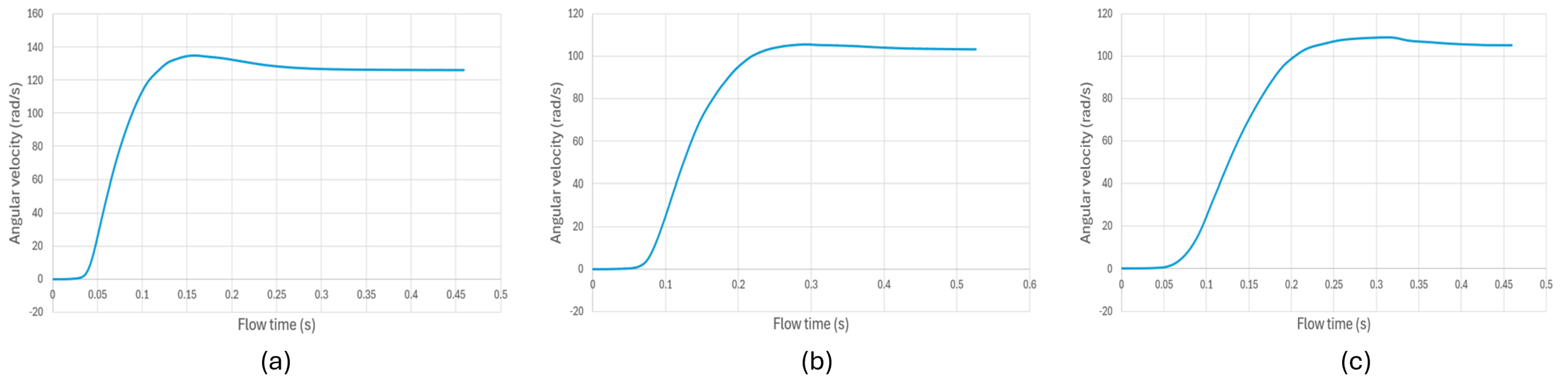
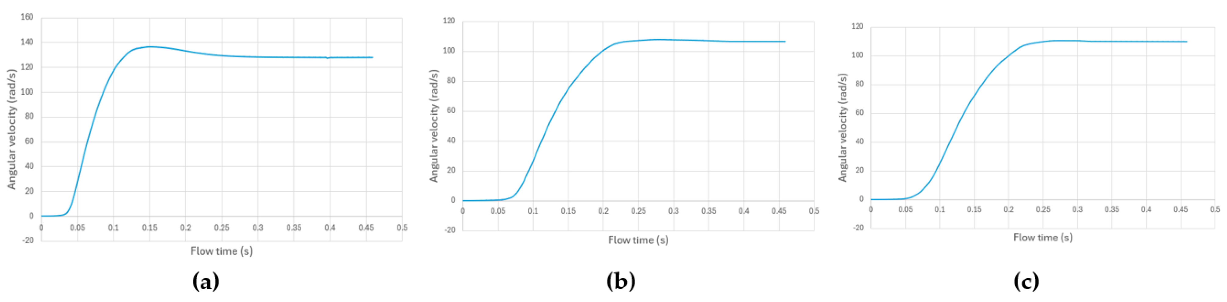
For the transient analysis of the turbine’s angular velocity, a total of 45,000 iterations were conducted with a timestep () of 0.001 s, ensuring a high temporal resolution to capture the dynamic response of the system. The results for the three cases exhibit consistent ascending trends, indicating a coherent acceleration phase followed by stabilization. In Figure 24a, the rotor experiences a rapid acceleration phase, reaching a peak velocity of approximately 140 rad/s within the first 0.125 s of simulation. This sharp increase suggests an initial impulsive torque. However, the system subsequently undergoes a stabilization phase, where the velocity settles at 126.1 rad/s, indicating that the initial peak is transient and influenced by early flow instabilities. In contrast, Figure 24b,c depict smoother acceleration curves, free of abrupt peaks, with a more gradual velocity increase until reaching a quasi-steady state at around 0.45 s. The final stabilized angular velocities in these cases are 103.5 rad/s and 105.2 rad/s, respectively, which are noticeably lower than in case (a). The absence of sharp peaks in cases (b) and (c) suggests that the flow characteristics lead to a more progressive energy transfer, due to reduced mass flow rate and impact velocities on the rotor blades, as previously discussed in the previous paragraph.
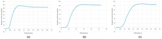
Figure 24.
Transient state results from angular velocity of the internal rotor using SST k- turbulent model, supplying flow at 350 kPa from both manifolds (a), lower manifold, (b) and upper manifold (c).
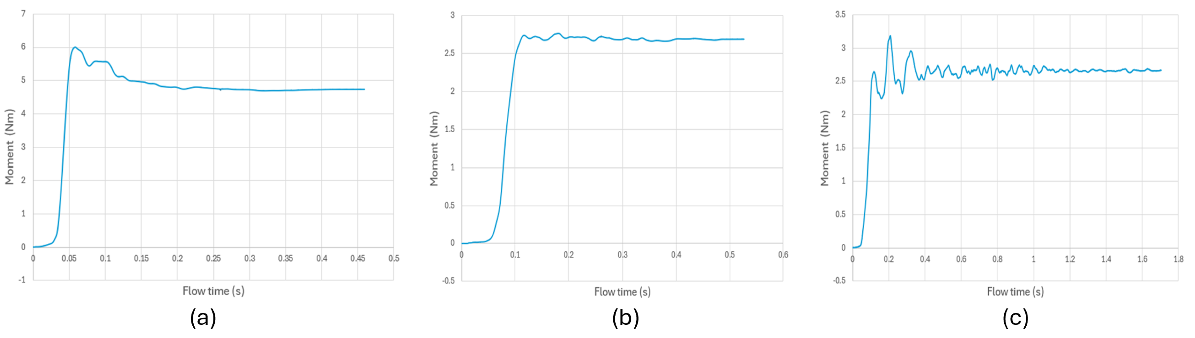
The obtained moment graphs reflect trends consistent with the previous results. In the first case, illustrated in Figure 25a, the dual-feed system reaches a maximum peak of approximately 6 Nm during the first 0.08 s of simulation. Subsequently, the moment drops to 5.5 Nm after 0.1 s and finally stabilizes at 4.73 Nm. Figure 25b, on the other hand, shows a lower performance, with a peak of 2.75 Nm in the initial 0.1 s. From that point on, small oscillations are observed that gradually converge until reaching a stable value of 2.69 Nm. Finally, in case (c) it was necessary to increase the number of iterations to almost 90,000 due to the erratic behavior obtained at the initial moments (see Figure 25c), where it was possible to capture a maximum peak of 3.2 Nm at moment 0.2. This oscillatory pattern persists until approximately 1 s of simulation, at which point the oscillations are considerably attenuated, stabilizing at 2.67 Nm. All the results obtained in quasi-steady state are summarized in Table 4.
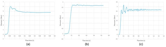
Figure 25.
Transient state results from moment of the internal rotor using SST k- turbulent model, supplying flow at 350 kPa from both manifolds (a), lower manifold (b) and upper manifold (c).
Figure 26 shows the angular velocity obtained using the k- turbulence model. A similar behavior is observed compared to the previous case with the SST k- model, reaching a peak value of 136.4 rad/s before stabilizing in a quasi-steady state from 0.25 s of simulation, with a final angular velocity of 127.7 rad/s (shown in Figure 26a), resulting in a difference of 1.6 rad/s compared to the SST k- model.
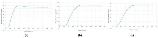
Figure 26.
Transient state results from angular velocity of the internal rotor using k- turbulent model, supplying flow at 350 kPa from both manifolds (a), lower manifold (b), and upper manifold (c).
On the other hand, due to the lower flow rate passing through the system in cases (b) and (c), the stabilization time is longer, occurring after 0.3 s of simulation. In these cases, Figure 26b,c show very similar curves, where the final stabilized angular velocities are 106.4 rad/s and 109.7 rad/s, respectively. The difference in angular velocity between both turbulence models is due to how each one predicts energy dissipation and stress distribution on the rotor. The k- model, designed for fully turbulent flows, tends to underestimate dissipation in regions of strong curvature and rotation, leading to a more uniform pressure field and lower resistance to rotor movement. As a result, a greater fraction of the fluid’s energy is transferred to the rotor, slightly increasing its angular velocity. In contrast, the SST k- model, being more sensitive to boundary layer effects and flow separation, captures pressure gradients and dissipation near the rotor surfaces more accurately. This results in a more pronounced shear stress field, increasing resistance to movement and slightly reducing the angular velocity compared to the k- model.
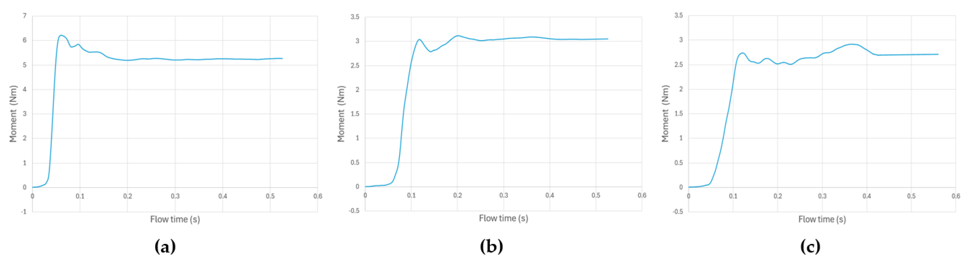
The results shown in Figure 27a indicate that the maximum peak torque obtained was 6.11 Nm at 0.07 s of simulation. A decreasing trend is observed immediately after, reaching 5.7 Nm at 0.1 s. From 0.2 s onward, the first signs of stabilization appear, with the torque reaching 5.2 Nm, and finally, a quasi-steady state is achieved at 0.3 s, with a stabilized value of 5.27 Nm. Figure 27b shows significant differences compared to the SST k- model. The curve exhibits an increasing trend, followed by a slight drop at 0.14 s. After this point, the torque rises again until 0.2 s, surpassing 3 Nm, and then gradually stabilizes at 3.05 Nm. Finally, Figure 27c presents a more erratic behavior, where stabilization occurs at a considerably later stage. In this case, a steady state torque of 2.71 Nm is reached only after 0.4 s of simulation.
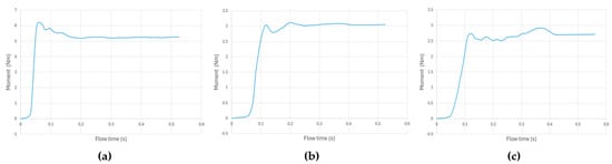
Figure 27.
Transient state results from moment of the internal rotor using SST k- turbulent model, supplying flow at 350 kPa from both manifolds (a), lower manifold (b), and upper manifold (c).
The results shown in Table 6 show significant changes in the mass flow rates obtained compared to the mathematical model calculated (3.5 kg/s), since it is shown that in the central zone of the swirl chamber low pressure zones form (shown in the previous results) causing the injection flow to be altered. These obtained data confirm the hypothesis made with the magnitude of the velocities in the expansion zone, because the fluid will be absorbed by the low pressures, which also directly impacts the mass flow rate. This fact in turn involves the fact that the torque obtained for case (a) is evidently maximized by the 5.795 and 5.835 kg/s recorded from SST k- and k- turbulence model, which also causes the slight differences between the angular velocities obtained: 126.1 rad/s and 127.7 rad/s, respectively.
Table 6.
Turbine operating conditions and performance based on the 3 cases analyzed.
Table 7 shows the mechanical power generated by the system which was calculated based on Equation (16). These data, together with the available hydraulic power, help to obtain the efficiency using Equation (17). Finally, it is observed that the maximum efficiency obtained is 29.4% and 32.9% (both manifolds fed), and this slight difference goes hand in hand with the counterflow found in the manifolds without hydraulic supply and the tetrahedral air core found in the area below the internal rotor. Both factors reduce the overall performance of the system because they do not contribute to the movement of the turbine. The other two cases (b) and (c) show quite similar behaviors where there is a very slight difference in mass flow rate, torque, and angular velocity, where it is observed that the k- model tends to overestimate the results obtained. Although there is no mathematical model, this comparison is useful to validate the operating conditions obtained numerically and to delimit them within an interval of interest. This also establishes the first step for future research involving experimental tests, where the most suitable model between the two can be defined according to the characteristics of the flow based on the geometry and the specific operating conditions of the turbine.
Table 7.
Turbine operating conditions and performance based on the 3 cases analyzed.
4.4. Varying Pressure Inlet Feeding Both Manifolds
Three additional cases were analyzed (d, e, and f), considering an inlet pressure to the atomizer of: 250, 300, and 400 kPa. These tests were carried out in order to verify the hydraulic consumption of the turbine and obtain its characteristic curve.
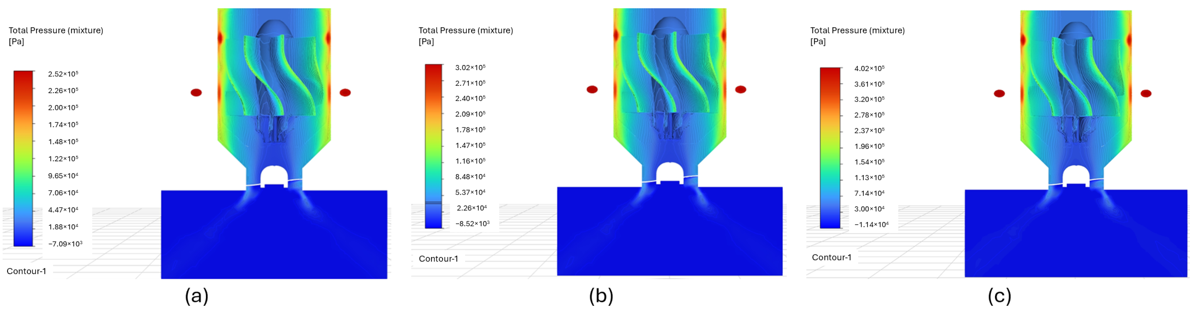
In all Figure 28, it can be observed that the pressure distribution is quite similar to the previously analyzed case (a), showing differences in the maximum and minimum magnitudes obtained. Such is the case of −7.09 kPa, −8.52 kPa, and −11.4 kPa, for Figure 28a,b,c, respectively. In this sense, it is curious that, when injecting a flow with higher pressure, the low-pressure zones become even more negative. This is easily justified by the exit velocity of the fluid, which directly affects the stabilizer blades. As the injection pressure increases, the exit velocity is also altered.

Figure 28.
Total pressure contour in the turbine system utilizing both manifolds, for 250 kPa (a), 300 kPa (b), and 400 kPa (c).
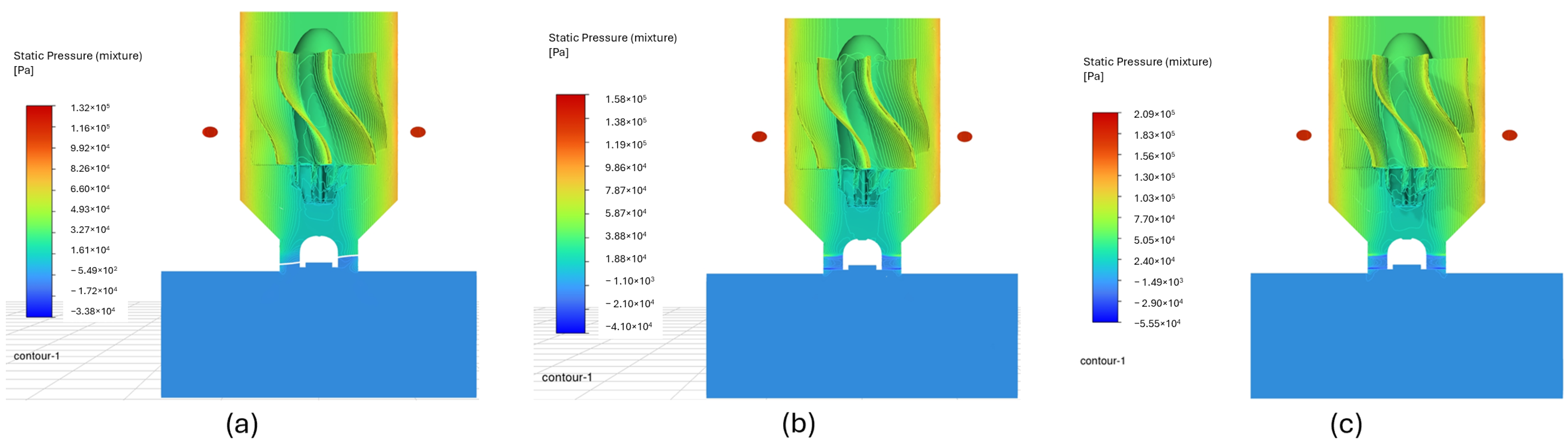
On the other hand, the analysis of static pressure distribution reveals a significant pressure gradient across the turbine’s internal components. As shown in Figure 29a, higher static pressures are concentrated around the walls of the swirl chamber, where the fluid follows a tangential trajectory. This region, shaded faintly in orange, exhibits pressures around 80 kPa, which is attributed to the centrifugal force generated by the rotational motion of the fluid. The pressure buildup in this area aligns with the classical behavior of swirling flows, where static pressure reaches a maximum near the outer periphery due to the conservation of angular momentum. Downstream, as the fluid approaches the contraction region, particularly near the stabilizer, a considerable pressure decay is observed. This effect is clearly depicted in Figure 29b,c, where the static pressure values drop significantly along the surfaces of the stabilizer blades. The recorded pressure ranges are [, ] kPa in case (b) and [, ] kPa in case (c), highlighting an intensification of the adverse pressure gradient. This pronounced drop is directly linked to the high fluid velocities induced by the convergent section of the outlet orifice, which accelerates the flow, reducing the static pressure according to Bernoulli’s principle.

Figure 29.
Static pressure contour in the turbine system utilizing both manifolds, for 250 kPa (a), 300 kPa (b), and 400 kPa (c).
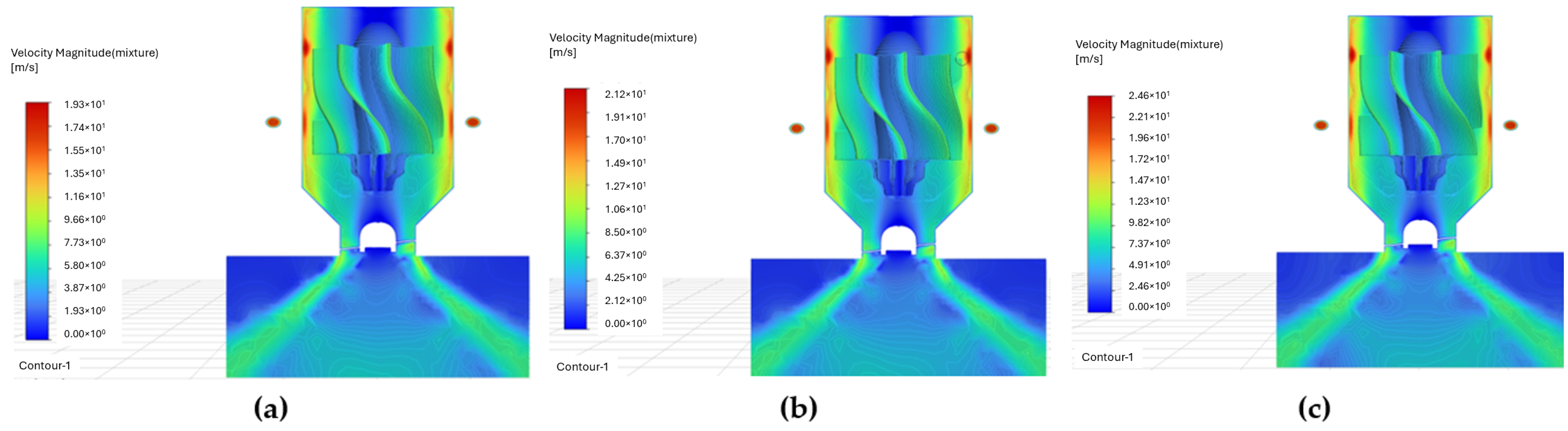
Figure 30 shows the velocity magnitude profile of the internal flow, which reveals a consistent trend: as the inlet pressure increases in the inlet channels, the velocity at the swirl chamber walls also increases in all three cases. However, it is especially relevant to observe the velocities in the contraction zone, near the stabilizer, since a considerable drop in static pressure was observed there. In this sense, three intervals of fluid exit velocities can be defined: [9.46–9.66] m/s, [10.4–10.6] m/s, and [11.7–12] m/s, corresponding to Figure 30a,b,c, respectively. These values highlight the behavior of the flow in a critical region, where the drop in static pressure in the contraction is reflected in the increase in fluid velocity, which is related to the principle of conservation of energy and the acceleration of the flow when passing through an area of smaller cross-section. Furthermore, the effects of the air core, which penetrates the stabilizer, contribute to a considerable decrease in the velocities in the upper area of the stabilizer and the lower part of the inner rotor (pre-stabilizer), which also impacts the pressure distribution in that area. In detail, the velocities in that area for the different cases vary between 0.19 and 1.55 m/s in Figure 30a, between 0.42 and 2.12 m/s in Figure 30b, and between 0.49 and 2.45 m/s in Figure 30c.
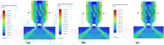
Figure 30.
Velocity magnitude contour in the turbine system utilizing both manifolds, for 250 kPa (a), 300 kPa (b), and 400 kPa (c).
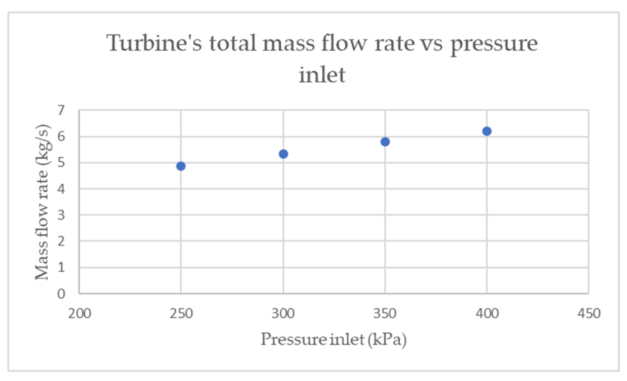
The mass flow obtained (Table 8 and Figure 31) shows a logical increasing tendency, the lowest of all referring to case (d) has a value of 4.866 kg/s, a value much higher than the design flow (3.5 kg/s). As previously detailed, this is caused by the considerable low pressures generated in the center of the atomizer and in the structure of the stabilizer, which causes a flow suction effect.
Table 8.
Numerical mass flow rate obtained.
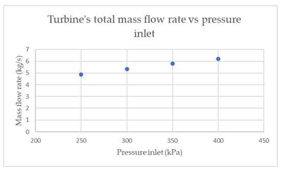
Figure 31.
Hydraulic system consumption in relation to fluid injection pressure for both manifolds.
5. Conclusions
The objective of this study was to evaluate the potential of centrifugal atomizers as energy generation systems, focusing on their internal flow dynamics and hydraulic performance under varying configurations. In this study, the mesh was designed following best practices for turbulence modeling, ensuring proper near-wall resolution through the criterion. While a formal grid convergence index (GCI) analysis was not conducted, the selected mesh provides stable and physically consistent results, aligning with the comparison of results obtained using two turbulence models. Numerical simulation tests were conducted to analyze factors such as mass flow rate, pressure response, and mechanical efficiency, providing valuable insights into the viability of this technology for renewable energy applications. The simulations confirmed that these systems can produce mechanical energy while maintaining uniform spray effects, despite minor flow deformations. This demonstrates their potential for integration into renewable energy solutions.
Among the feeding configurations tested, the dual manifold setup emerged as the most efficient, achieving an efficiency of 29.4 and 32.9%, using the SST k- and k- turbulence model, respectively. It was observed that this configuration maximized mass flow, torque and angular velocity (126.1 and 127.7 rad/s). To evaluate the performance of the proposed design, it is important to compare it with conventional hydraulic turbines and identify its differences and potential improvements. Currently, turbines such as Francis or Pelton have well-documented efficiencies (85–90%), but their performance depends on specific conditions. For example, Pelton turbines are very efficient for high head heights (greater than 300 m), while the ideal operating range for Francis turbines is at flow rates of around 0.2–10 m3/s. Although efficiency in this system may be lower than that of some traditional turbines, its optimized flow distribution design could make it more adaptable to variations in flow rate without significant efficiency loss. Unlike a Pelton turbine, which requires high-pressure water jets, this system aims to enhance flow utilization through a refined inlet channel geometry. Another important aspect to consider is manufacturing, as many turbines require high-precision components and costly materials, whereas this design could be simpler and more cost-effective to produce. Overall, this comparison helps contextualize where the system stands in the field of energy generation, highlighting its advantages and identifying areas for further optimization.
Regarding the turbine design, it can be stated that it was effective due to the fluid behavior observed around the upper dome, which helps direct the water portions towards the inner rotor blades (Figure 19). Additionally, for cases (b) and (c), the pre-stabilizer effectively redirected the particles in the small air core towards the outlet orifice. However, the efficiency in both cases was slightly reduced by the appearance of backflows at the inlets of the channels without hydraulic supply, which decreased the usable mass flow. Another important factor that influenced the performance was the abrupt pressure drop around the inner rotor. While this positively affected the magnitude of the fluid velocity in the expansion zone, it did not have the same effect in the area adjacent to the surface of its blades, where significantly lower values were observed compared to case (a).
Some key aspects to improve to optimize system efficiency are as follows:
- Supply fluid using both manifolds in order to reduce hydraulic losses caused by the aforementioned counterflow.
- Increase the length of the turbine to better match the height of the swirl chamber, thus taking full advantage of the velocity profile adjacent to the walls.
- Ensure that the inner rotor blades are even closer to the swirl chamber so that they can be aligned directly with the liquid expansion zone. Similarly, it is possible to increase the number of manifolds and evaluate the turbine performance under these new conditions.
Finally, the response to pressure variations (between 250 and 400 kPa) was consistent, with a proportional increase in mass flow from 4.87 to 6.21 kg/s, respectively. This behavior facilitated the development of the turbine characteristic curve, which is an essential tool to understand its performance and ensure its efficient integration into a hydraulic generation system.
Author Contributions
Conceptualization, D.C., A.U., J.R., D.V., C.R., W.N., G.Z. and G.R.; methodology, J.R. and D.V.; software, D.C., A.U. and J.R.; validation, D.C., A.U. and J.R.; formal analysis, J.R.; investigation, D.C., A.U., W.N. and G.Z.; data curation, D.C., A.U. and J.R.; writing—original draft preparation, D.C., A.U., J.R., D.V., C.R., W.N., G.Z. and G.R.; writing—review and editing, D.C., A.U., J.R. and G.Z.; visualization, D.C., A.U. and J.R.; supervision, J.R. and G.Z.; project administration, J.R.; funding acquisition, J.R. and C.R. All authors have read and agreed to the published version of the manuscript.
Funding
The authors would like to thank to the “Dirección de Investigación de la Universidad Peruana de Ciencias Aplicadas” for the support provided to carry out this research work through the UPC-EXPOST-2025-1 incentive.
Data Availability Statement
The original contributions presented in the study are included in the article, further inquiries can be directed to the corresponding author.
Conflicts of Interest
The authors declare no conflicts of interest.
Nomenclature
| A | Geometrical characteristics parameter of pressure-swirl atomizer |
| Equivalent geometrical characteristics parameter due to viscosity of | |
| swirl atomizers | |
| C | Aperture coefficient |
| Discharge coefficient | |
| Equivalent discharge coefficient | |
| Skin friction coefficient | |
| D | Turbine diameter |
| Inlet slot cross-sectional area | |
| g | Gravity acceleration |
| H | Hydraulic head |
| Channel inlet length | |
| N | Revolutions per minute |
| n | Number of inlet channels |
| Mass flow rate (kg/s) | |
| Differential pressure | |
| Hydraulic power available | |
| Mechanical power | |
| Q | Flow rate (/s) |
| Swirl chamber radius | |
| Distance from the center of the atomizer to the center of the inlet channel | |
| Air core radius | |
| Exit hole radius | |
| Inlet channel radius | |
| T | Torque |
| U | Axial velocity |
| W | Radial velocity |
| Dimensionless distance to wall | |
| Greek Symbols | |
| Spray semi-angle | |
| Swirl angle | |
| Loss coefficient | |
| Mechanical efficiency | |
| Filling coefficient | |
| Tilt angle | |
| Blasius resistance coefficient | |
| Liquid absolute viscosity | |
| Helix angle | |
| Liquid density | |
| Liquid kinematic viscosity | |
| Angular velocity (rad/s) | |
| Wall shear stress | |
| Subscripts | |
| a | Air core |
| eq | Equivalent parameter due to hydraulic losses |
| inj | Parameter related to inlet channels |
| in | Parameter related to atomizer inlet |
| o | Atomizer orifice outlet |
| out | Parameter related to atomizer outlet |
| S | Swirl chamber |
| tot | Total |
References
- Song, W.; Hwang, J.; Koo, J. Atomization of Gelled Kerosene by Multi-Hole Pintle Injector for Rocket Engines. Fuel 2021, 285, 119212. [Google Scholar]
- Chen, C.; Yang, Y.; Yang, S.; Gao, H. The Spray Characteristics of an Open-End Swirl Injector at Ambient Pressure. Aerosp. Sci. Technol. 2017, 67, 78–87. [Google Scholar]
- Ronceros Rivas, J.R.; Pimenta, A.P.; Lessa, J.S.; Ronceros Rivas, G.A. An Improved Theoretical Formulation for Sauter Mean Diameter of Pressure-Swirl Atomizers Using Geometrical Parameters of Atomization. Propuls. Power Res. 2022, 11, 240–252. [Google Scholar]
- Kang, Z.; Wang, Z.; Li, Q.; Cheng, P. Review on Pressure Swirl Injector in Liquid Rocket Engine. Acta Astronaut. 2018, 145, 174–198. [Google Scholar]
- Zhang, T.; Dong, B.; Chen, X.; Qiu, Z.; Jiang, R.; Li, W. Spray Characteristics of Pressure-Swirl Nozzles at Different Nozzle Diameters. Appl. Therm. Eng. 2017, 121, 984–991. [Google Scholar] [CrossRef]
- Jedelský, J.; Malý, M.; Vankeswaram, S.K.; Zaremba, M.; Kardos, R.; Csemány, D.; Červenec, A.; Józsa, V. Effects of Secondary Breakup, Collision Dynamics, Gravity and Evaporation on Droplet Size Distribution in a Pressure-Swirl JET A-1 Spray. Fuel 2024, 359, 130103. [Google Scholar]
- Urbán, A.; Katona, B.; Malý, M.; Jedelský, J.; Józsa, V. Empirical Correlation for Spray Half Cone Angle in Plain-Jet Airblast Atomizers. Fuel 2020, 277, 118197. [Google Scholar] [CrossRef]
- Ronceros, J.; Raymundo, C.; Ayala, E.; Rivera, D.; Vinces, L.; Ronceros, G.; Zapata, G. Study of Internal Flow in Open-End and Closed Pressure-Swirl Atomizers with Variation of Geometrical Parameters. Aerospace 2023, 10, 930. [Google Scholar] [CrossRef]
- Ma, D.; Chang, S.; Wu, K.; Yang, C. Experimental Investigation on the Characteristics of Film Thickness and Temperature on the Heated Surface during Spray Cooling. Sustain. Energy Technol. Assess. 2022, 51, 101871. [Google Scholar]
- Rivas, J.R.; Pimenta, A.P.; Rivas, G.R. Development of a mathematical model and 3D numerical simulation of the internal flow in a conical swirl atomizer. J. At. Sprays 2014, 24, 97–114. [Google Scholar]
- Abramovich, G.N. The Theory of Swirl Atomizers. In Industrial Aerodynamics; BNT ZAGI: Moscow, Russia, 1944. [Google Scholar]
- Khavkin, Y.I. The Theory and Practice of Swirl Atomizers; CRC Press: New York, NY, USA, 2004. [Google Scholar]
- Kessaev, K.; Kupatenkov, V.D. Injectors Design for Liquid Rocket Engines. In Book of Fundamental Course in Engine Design; CTA/IAE/ASA-P: São José dos Campos, Brazil, 1997; pp. 31–49. [Google Scholar]
- Bazarov, V.; Yang, V.; Puri, P. Design and Dynamics of Jet and Swirl Injectors. In Liquid Rocket Thrust Chambers: Aspects of Modeling, Analysis, and Design; Lincoln Laboratory: Lexington, MA, USA, 2004; Volume 200, pp. 19–103. [Google Scholar]
- Rivas, J.R. Modelo Matemático e Simulação Numérica da Atomização de Líquidos em Injetores Centrífugos de uso Aeroespacial. Ph.D. Dissertation, Instituto Tecnológico de Aeronáutica, São José dos Campos, Brazil, 2015. [Google Scholar]
- Chen, J.; Yang, H.X.; Liu, C.P.; Lau, C.H.; Lo, M. A Novel Vertical Axis Water Turbine for Power Generation from Water Pipelines. Energy 2013, 54, 184–193. [Google Scholar]
- Naghizadeh, R.A.; Jazebi, S.; Vahidi, B. Modeling Hydro Power Plants and Tuning Hydro Governors as an Educational Guideline. Int. Rev. Model. Simul. 2012, 5, 123–130. [Google Scholar]
- Liu, J.; Feng, X.; Liang, H.; Zhang, W.; Hui, Y.; Xu, H.; Yang, C. Prediction of Atomization Characteristics of Pressure Swirl Nozzle with Different Structures. Chin. J. Chem. Eng. 2023, 63, 171–184. [Google Scholar]
- Li, X.; Du, J.; Wang, L.; Fan, J.; Peng, X. Effects of Different Nozzle Materials on Atomization Results via CFD Simulation. Chin. J. Chem. Eng. 2020, 28, 362–368. [Google Scholar]
- Cejpek, O.; Malý, M.; Bělka, M.; Jedelský, J. Replication of Pressure Swirl Atomizer by 3D Printing and Influence of Surface Roughness on the Atomization Quality. MATEC Web Conf. 2020, 328, 01007. [Google Scholar]
- Bak, C. 3-Aerodynamic Design of Wind Turbine Rotors. In Advances in Wind Turbine Blade Design and Materials; Brøndsted, P., Nijssen, R.P.L., Eds.; Woodhead Publishing Series in Energy; Woodhead Publishing: Cambridge, UK, 2013; pp. 59–108. [Google Scholar]
- Ronceros, J.; Raymundo, C.; Zapata, G.; Namay, W.; Ronceros, G. Comprehensive Theoretical Formulation and Numerical Simulation of the Internal Flow in Pressure-Swirl Atomizers Type Screw-Conveyer. Energies 2024, 17, 5414. [Google Scholar] [CrossRef]
- Arriaga, I.; Sayán, J.; Ronceros, J.; Klusmann, M.; Albatrino, R.; Raymundo, C.; Zapata, G.; Ronceros, G. Study of Internal Flow in a Liquid Nitrogen Flow Decelerator Through Swirl Effect Consisting of a Jet-Type Cryogenic Injection System for Food Freezing. Fluids 2024, 9, 302. [Google Scholar] [CrossRef]
- Barrera, E.F.; Aguirre, F.A.; Vargas, S.; Martínez, E.D. Influencia del Y Plus en el Valor del Esfuerzo Cortante de Pared a través Simulaciones empleando Dinámica Computacional de Fluidos. Inf. Tecnol. 2018, 29, 291–302. [Google Scholar]
- ANSYS. ANSYS Meshing User’s Guide, Release 13.0; ANSYS, Inc.: Canonsburg, PA, USA, 2008. [Google Scholar]
- Oladosu, T.L.; Koya, O.A. Numerical Analysis of Lift-Based in-Pipe Turbine for Predicting Hydropower Harnessing Potential in Selected Water Distribution Networks for Waterlines Optimization. Eng. Sci. Technol. Int. J. 2018, 21, 672–678. [Google Scholar] [CrossRef]
- Shahverdi, K.; Loni, R.; Maestre, J.M.; Najafi, G. CFD Numerical Simulation of Archimedes Screw Turbine with Power Output Analysis. Ocean. Eng. 2021, 231, 108718. [Google Scholar]
- Velásquez, L.; Rubio-Clemente, A.; Chica, E. Numerical and Experimental Analysis of Vortex Profiles in Gravitational Water Vortex Hydraulic Turbines. Energies 2024, 17, 3543. [Google Scholar] [CrossRef]
- Li, D.; Wang, H.; Xiang, G.; Gong, R.; Wei, X.; Liu, Z. Unsteady Simulation and Analysis for Hump Characteristics of a Pump Turbine Model. Renew. Energy 2015, 77, 32–42. [Google Scholar]
- Jubaer, H.; Afshar, S.; Xiao, J.; Chen, X.D.; Selomulya, C.; Woo, M.W. On the Effect of Turbulence Models on CFD Simulations of a Counter-Current Spray Drying Process. Chem. Eng. Res. Des. 2019, 141, 592–607. [Google Scholar] [CrossRef]
- Hu, X.; Zhang, L. Vortex Cascade Features of Turbulent Flow in Hydro-Turbine Blade Passage with Complex Geometry. Water 2018, 10, 1859. [Google Scholar] [CrossRef]


Disclaimer/Publisher’s Note: The statements, opinions and data contained in all publications are solely those of the individual author(s) and contributor(s) and not of MDPI and/or the editor(s). MDPI and/or the editor(s) disclaim responsibility for any injury to people or property resulting from any ideas, methods, instructions or products referred to in the content. |
© 2025 by the authors. Licensee MDPI, Basel, Switzerland. This article is an open access article distributed under the terms and conditions of the Creative Commons Attribution (CC BY) license (https://creativecommons.org/licenses/by/4.0/).