Impact of Addition of a Newtonian Solvent to a Giesekus Fluid: Analytical Determination of Flow Rate in Plane Laminar Motion

Abstract

In this study, the influence of the presence of a Newtonian solvent on the flow of a Giesekus fluid in a plane channel or fracture is investigated with a focus on the determination of the flow rate for an assigned external pressure gradient. The pressure field is nonlinear due to the presence of the normal transverse stress component. As expected, the flow rate per unit width $Q^{\prime }$ is larger than for a Newtonian fluid and decreases as the solvent increases. It is strongly dependent on the viscosity ratio $\epsilon$ ($0\le \epsilon \le 1$), the dimensionless mobility parameter $\beta$($0\le \beta \le 1$) and the Deborah number $De$, the dimensionless driving pressure gradient. The degree of dependency is notably strong in the low range of $\epsilon$. Furthermore, $Q^{\prime }$ increases with $De$ and tends to a constant asymptotic value for large $De$, subject to the limitation of laminar flow. When the mobility factor $\beta$ is in the range $\left[0.5÷1\right]$, there is a minimum value of $\epsilon$ to obtain an assigned value of $De$. The ratio $U_N/U$ between Newtonian and actual mean velocity depends only on the product $\sqrt{\beta }De$, as for other non-Newtonian fluids.

1. Introduction

Industrial and environmental applications involving viscoelastic fluids are manifold, including injection molding, filament stretching, plastic extrusion, container filling, flow of slurry suspensions and oil well drilling. In addition, their use is widespread in heat transfer equipment, inkjet printers, pharmacology and the food industry, as noted by Caglar Duvarci et al. [1]. The rheological behavior of viscoelastic fluids is complex, showing non-linear relationships between stress and strain as opposed to the proportionality relation typical of Newtonian fluids; hence, practical problems involving them are difficult to solve analytically due to their complexity, and analytical solutions for the velocity field and flow rate are scarce even for simple geometries. This prompted the use of numerical methods, which constitute an irreplaceable tool for advanced simulation of non-Newtonian fluid flows.

The viscoelastic constitutive equation, typically associated with complex polymers, spans different degrees of complexity. Among possible choices, the Giesekus model is particularly appealing for its solid physical foundations (Giesekus [2,3]) and incorporates three physical parameters: the viscosity, the relaxation time and the mobility factor. While the former two times are quite typical in non-Newtonian fluid mechanics, this is less true for the mobility factor, a dimensionless quantity ranging between zero and unity. Debbaut and Burhin [4] and Calin et al. [5] present an experimental determination of the mobility factor associated with the Giesekus model by performing multiple experiments to characterize a high-density polyethylene fluid. Further experiments were performed by Rehage and Fuchs [6], both under steady-state shear flow and an oscillating shear regime. The aim of these experiments was to ascertain the model consistency when compared with experimental data; the author found a very good agreement under steady state flow, while the fluid showed instability under oscillating pressure gradients of large amplitude.

The Giesekus model allows derivation of analytical solutions for plane Couette and Poiseuille flows, as first shown, to the best of our knowledge, by Yoo and Choi [7], who individuated a clear distinction between two ranges of variation of the mobility parameter and defined for both a bound in terms of the Deborah number; beyond each bound, no solution is possible. The solutions for Poiseuille flow, including the possible viscosity contribution of the solvent, were analyzed by Schleiniger and Weinacht [8] who determined, though in implicit form, the solution with physical significance for plane and axisymmetric flow.

Available closed-form solutions are typically limited by the linear approximation adopted, and hence are valid in a small range of parameters. In contrast to these, Daprà and Scarpi [9] provide a semi-analytical solution for a plane Poiseuille flow: their approach applies to the entire range of values of the physical and geometric parameters involved. A semi-analytical solution for channel flow with wall slip was derived by Ferrás et al. [10].

When a solvent is added to the viscoelastic fluid, the effects of the non-linear terms in the constitutive equation are magnified; this increases the mathematical complexities intrinsic in the rheology and presents more challenges for finding analytical solutions for simple geometries. Cruz et al. [11] contribute a relevant example for flow in circular pipe with reference to two different polymer constitutive equations, the PTT and FENE-P models, while the solvent is conceptualized as a Newtonian fluid; the authors derived a solution for both axisymmetric and plane geometry. Araujo et al. [12] provide another example in the literature of complete solution without simplification considering a solvent addition, where the LPTT viscoelastic rheology is adopted to infer a semi-analytical solution for the streamwise velocity component and the components of the extra-stress tensor.

For flow of a Giesekus flow between parallel plates, Silva Furlan et al. [13] propose an approach alternative to the classical one, in which the independent variable is the distance from the center of the channel. According to their approach, a component of the stress tensor is first chosen as the independent variable; subsequently, rewriting the system of equations and solving it allows for comparing the results with those of Schleiniger and Weinacht [8] and then with a full numerical solution of the momentum balance and constitutive equations. This leads to an analytical determination of the components of the stress tensor, and to the numerical integration of the velocity profile via a higher-order method.

The effect of the contribution of a Newtonian solvent to the parallel plate flow of a Giesekus fluid is revisited in the semi-analytical solution by Daprà and Scarpi [14]. In this paper, the velocity profile is determined as a function of three parameters: the mobility factor, the Deborah number and the ratio between the solvent viscosity and the total viscosity. The present work significantly advances their contribution by analytically determining the flow rate. For assigned pressure gradient, it is observed that (i) the flow rate for the Giesekus fluid is seen to be larger than for the Newtonian one; (ii) the flow rate decreases as the solvent increases. The implications of these theoretical findings have practical implications in designing more efficient industrial processes. Good references on non-Newtonian fluids are Bird et al. [15] and Deville and Gatski [16], where the Giesekus model is specifically mentioned.

The organization of this paper is as follows: Section 2 presents the problem formulation and its general solution, Section 3 gives explicit expressions for the velocity field, while the evaluation of the flow rate is presented in Section 4 and the friction factor in Section 5. The numerical results are discussed in Section 6, and Section 7 closes the paper.

2. Problem Setting and Solution

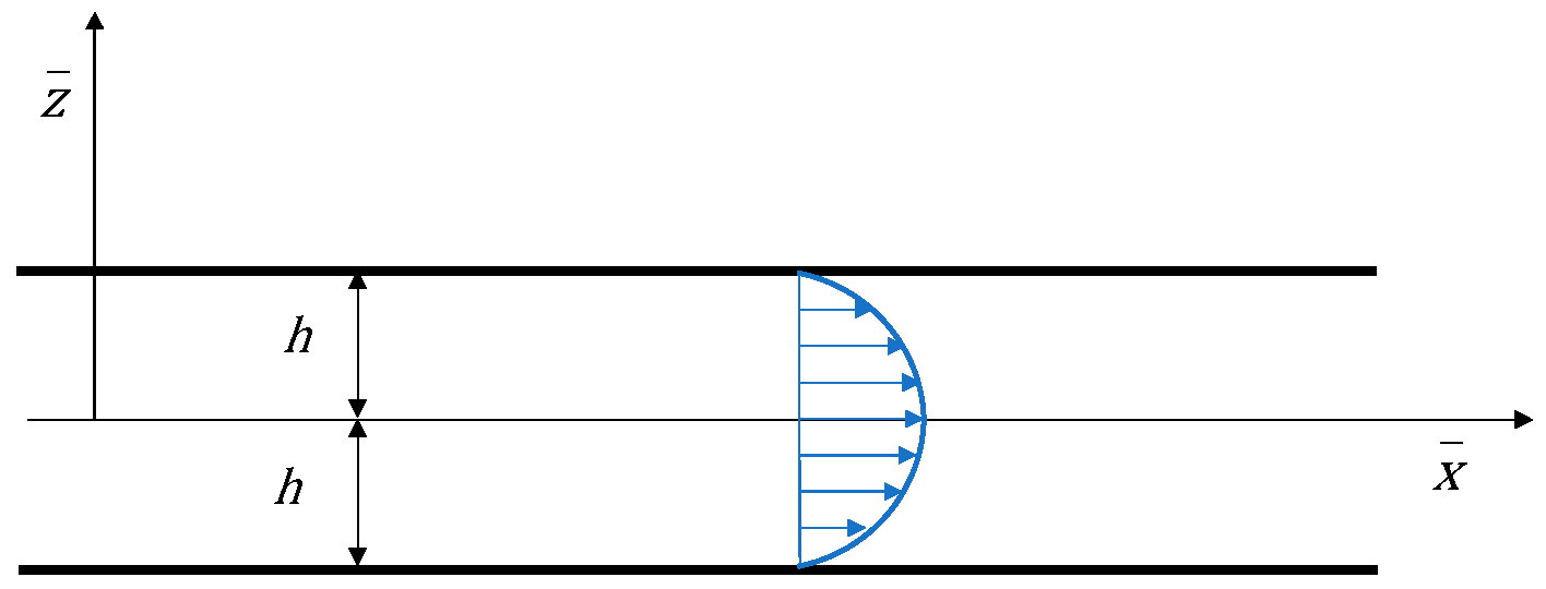
A constant pressure gradient $P=-\partial \overline{p}/\partial \overline{x}$ acts on an incompressible Giesekus fluid filling a plane layer of thickness $2h$, $-h\le \overline{z}\le h$ (see Figure 1); the laminar steady motion in the direction of $\overline{x}$ axis is described using the continuity and momentum equations, reading in general form $\nabla ·v=0$ and $-\nabla \overline{p}+\nabla ·T=0$, where $v$ is the velocity vector, $\overline{p}$ the pressure and $T$ the total stress tensor.

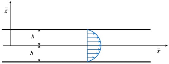
Figure 1. Flow configuration.

The total stress tensor for a Giesekus fluid with non-zero solvent viscosity can be written as

$$T={T_p+T}_s,$$

(1)

where the first part refers to the polymer contribution and satisfies the equation

$$T_p+\lambda \left[{\displaystyle \frac{\partial T_p}{\partial \overline{t}}}+v·\nabla T_p-T_p·\nabla v-{\left(\nabla v\right)}^T·T_p\right]+{\displaystyle \frac{\lambda \beta }{\mu }}{T}_p·T_p=\mu \left[\nabla v+{\left(\nabla v\right)}^T\right]$$

(2)

where $\mu$ is the zero-shear rate viscosity of the polymer, $\lambda$ the stress relaxation time and $\beta$ the dimensionless mobility parameter ($0\le \beta \le 1$).

With reference to the specific 1-D problem, the above equations become in dimensionless form:

$${\displaystyle \frac{du}{dx}}=0,$$

(3)

$$-{\displaystyle \frac{\partial p}{\partial x}}+\nabla ·\left({\tau }_p+{\tau }_s\right)=-{\displaystyle \frac{\partial p}{\partial x}}+\nabla ·{\tau }_p+\epsilon {\nabla }^{2}u=0,$$

(4)

where the non-dimensional quantities are as follows: $x=\overline{x}/h$, $z=\overline{z}/h$, the vector velocity is $u=v\left(\mu +\eta \right)/\left(P{h}^2\right)$, $\eta$ is the viscosity of the solvent $p=\overline{p}/\left(Ph\right)$ is the pressure, $t=\overline{t}Ph/\left(\mu +\eta \right)$ is the time, $\epsilon =\eta /\left(\mu +\eta \right)$ is the viscosity ratio with $0\le \epsilon \le 1$. The non-dimensional stress tensor is $\tau =T/\left(Ph\right)$. The non-dimensional stress component ${\tau }_p$ for a Giesekus fluid with non-zero solvent viscosity refers to the polymer contribution and satisfies the equation

$${\tau }_p+De\left(1-\epsilon \right)\left[{\displaystyle \frac{\partial {\tau }_p}{\partial t}}+u·\nabla {\tau }_p{-\tau }_p·\nabla u-{\left(\nabla u\right)}^T·{\tau }_p\right]+\beta De{\tau }_p·{\tau }_p=\left(1-\epsilon \right)[\nabla u+{\left(\nabla u\right)}^T].$$

(5)

Here, $\lambda$ is the stress relaxation time of the polymer, $\beta$ the dimensionless mobility parameter ($0\le \beta \le 1$) and $De=\lambda Ph/\mu$ is the Deborah number. $De$ encloses both physical parameters of the polymer, viscosity and relaxation time and the pressure gradient, which gives rise to the motion. The non-dimensional solvent contribution to the total stress is

$${\tau }_s=\epsilon \left[\nabla u+{\left(\nabla u\right)}^T\right].$$

(6)

For steady Poiseuille flow, the continuity Equation (3) is verified, and the momentum Equation (4) has two scalar components, as reported below. All the quantities depend only on $z$, except for $p=p\left(x,z\right)$ which depends linearly on $x$.

$$1+{\tau }_{pxz}^{\prime }=-\epsilon u\prime \prime$$

(7)

$${\displaystyle \frac{\partial p}{\partial z}}+{\mathsf{\tau }}_{pzz}^{\prime }=0$$

(8)

where a prime indicates $d/dz$. Equation (8) allows to write $p\left(x,z\right)$ as

$$p\left(x,z\right)=p_0-x-{\tau }_{pzz}$$

here $p_0$ is the assigned pressure at a given point, e.g., at $\left(x,z\right)=\left(\mathrm{0,0}\right)$.

The non-zero components of Equations (5) and (6) are

$${\tau }_{pxx}-2De{\tau }_{pxz}\left(1-\epsilon \right)u^{\prime }+\beta De\left({\tau }_{pxx}^2+{\tau }_{pxz}^2\right)=0,$$

(9)

$${\tau }_{pzz}+\beta De\left({\tau }_{pxz}^2+{\tau }_{pzz}^2\right)=0,$$

(10)

$${\tau }_{pxz}-De{\tau }_{pzz}{\left(1-\epsilon \right)u}^{\prime }+\beta De{\tau }_{pxz}\left({\tau }_{pxx}+{\tau }_{pzz}\right)={\left(1-\epsilon \right)u}^{\prime },$$

(11)

$${\tau }_{sxz}=\epsilon {\displaystyle \frac{\partial u}{\partial z}}.$$

(12)

As $\beta \to 0$ and $\epsilon =0$, Giesekus model reduces to the upper convected Maxwell model.

The flow field is symmetrical, so only the region defined by $-1\le z\le 0$ can be analyzed; the appropriate boundary conditions are

$$u\left(-1\right)=0,$$

(13)

$${\left.{\displaystyle \frac{du}{dz}}\right|}_{z=0}=0.$$

(14)

Solving Equation (14) with respect to ${\tau }_{pzz}$ gives

$${\tau }_{pzz}={\displaystyle \frac{-1\pm \sqrt{1-4{\beta }^2{De}^2{\tau }_{pxz}^2}}{2\beta De}},$$

(15)

where, obviously, the argument of the square root must be non-negative. According to Schleiniger and Weinacht [8], to have a stable behavior, the positive sign should be taken in Equation (15). The other polymeric normal stress ${\tau }_{pxx}$ can be obtained using Equation (11):

$${\tau }_{pxx}={\displaystyle \frac{\left(1-\epsilon \right)u\prime \left(1+De{\tau }_{pzz}\right)}{\beta De{\tau }_{pxz}}}-{\displaystyle \frac{1+\beta De{\tau }_{pzz}}{\beta De}}$$

(16)

therefore, both normal stresses can be expressed as a function of tangential stress.

The integration of Equation (7) allows to write

$$z=-\left({\tau }_{pxz}+\epsilon u^{\prime }\right).$$

(17)

Based on Equations (9)–(11) and some algebraic steps given in detail in Daprà and Scarpi [14], the equation for $u^{\prime }$ is as follows:

$$\begin{gathered} {u^{\prime }}^2{\left(1-\epsilon \right)}^2{\left({\tau }_{pxz}^2{De}^2\beta -1+\beta \right)}^2-u^{\prime }{\tau }_{pxz}\left(1-\epsilon \right)\left[{\tau }_{pxz}^2{De}^2\beta (8{\beta }^2-8\beta +1)-\beta +1\right] \\ +{\tau }_{pxz}^4{De}^2{\beta }^2{\left(2\beta -1\right)}^2+{\tau }_{pxz}^2\beta \left(1-\beta \right)=0, \end{gathered}$$

(18)

which can be solved to give the only valid solution in the whole range of variation of $\beta$:

$$\begin{gathered} u^{\prime }={\displaystyle \frac{{\tau }_{pxz}}{2\left(1-\epsilon \right){\left({{\tau }_{pxz}}^2{De}^2\beta +\beta -1\right)}^2}} \\ \left[{{\tau }_{pxz}^{2}De}^2\beta (8{\beta }^2-8\beta +1)+1-\beta +(1-2\beta )\left({\tau }_{pxz}^2{De}^2\beta -\beta +1\right)\sqrt{1-4{\tau }_{pxz}^2{De}^2{\beta }^2}\right]. \end{gathered}$$

(19)

The shear stress of the polymer at the wall $\left(z=-1\right),$ ${\tau }_{pxz}\left(-1\right)$ can be expressed as a fraction of ${\tau }_{pxzmax}$, where ${\tau }_{pxzmax}={\displaystyle \frac{1}{2\beta De}}$ is the maximum value of tangential stress in (15). However, according to Yoo and Choi [7] and Giesekus [17], the condition that should apply if $0\le \beta \le 0.5$ is as follows: ${\tau }_{pxzmax}={\displaystyle \frac{1}{De}}\sqrt{{\displaystyle \frac{1-\beta }{\beta }}}$, i.e., ${\tau }_{pxzmax}={\displaystyle \frac{\delta }{De}}$ being $\delta =\sqrt{{\displaystyle \frac{1-\beta }{\beta }}}$ if $0\le \beta \le 0.5$ and $\delta ={\displaystyle \frac{1}{2\beta }}$ if $0.5\le \beta \le 1$.

The shear stress at the wall can be expressed as

$${\tau }_{pxz}\left(-1\right)={\displaystyle \frac{k\delta }{De}}$$

(20)

where $0\le k\le 1$ represents the ratio between the wall shear-stress of the fluid and its limit-value ${\tau }_{pxzmax}$. Substituting Equation (20) in Equation (19) gives

$$\begin{gathered} u^{\prime }\left(-1\right)={\displaystyle \frac{k\delta }{2De(1-\epsilon ){(k^2{\delta }^2\beta +\beta -1)}^2}} \\ \left[k^2{\delta }^2\beta (8{\beta }^2-8\beta +1)+1-\beta +(1-2\beta )(k^2{\delta }^2\beta -\beta +1)\sqrt{1-4k^2{\delta }^2{\beta }^2}\right] \end{gathered}$$

(21)

Equation (17) can be solved with respect to $u\prime$: recalling Equation (20), it gives

$$u^{\prime }\left(-1\right)=(1-k\delta /De)/\epsilon ,$$

(22)

and substituting Equation (21) in Equation (22), a relation between the Deborah number $De$ and $k$ is obtained:

$$\begin{gathered} De={\displaystyle \frac{k\delta }{2\left(1-\epsilon \right){[k^2\beta {\delta }^2-1+\beta ]}^2}} \\ \left\{2k^4{\beta }^2{\delta }^4\left(1-\epsilon \right)+k^2\beta {\delta }^2[8{\beta }^2\epsilon +4\beta \left(1-3\epsilon \right)+5\epsilon -4]-[\beta \left(4-3\epsilon \right)+\epsilon -2-2{\beta }^2\left(1-\epsilon \right)] \\ +\epsilon (1-2\beta )(k^2\beta {\delta }^2-\beta +1)\sqrt{1-4k^2{\beta }^2{\delta }^2}\right\}. \end{gathered}$$

(23)

The parameter $k$, representing the ratio between the wall shear-stress of the fluid and its limit-value ${\tau }_{pxzmax}$ is linked to Deborah number by Equation (23).

3. Calculation of the Velocity

By solving Equation (17) with respect to $u^{\prime }$, it follows that

$$u^{\prime }\left(z\right)=-{\displaystyle \frac{{\tau }_{pxz}+z}{\epsilon }}.$$

(24)

For any $z$, the shear stress ${\tau }_{pxz}$ can be written as ${\tau }_{pxz}\left(z\right)=m{\tau }_{pxz}\left(-1\right)=mk{\tau }_{max}=mk\delta /De$, with $-1\le m\le 1$; when $m=\pm 1$ it results $z=\mp 1;$ expressing $u^{\prime }$ and $z$ as a function of $m$ yields

$$u^{\prime }\left(z\right)={\displaystyle \frac{du}{dz}}={\displaystyle \frac{du}{dm}}{\displaystyle \frac{dm}{dz}}=-{\displaystyle \frac{1}{\epsilon }}\left({\displaystyle \frac{mk\delta }{De}}+z\left(m\right)\right)$$

(25)

and thus

$$u\left(m\right)=-{\displaystyle \frac{1}{\epsilon }}\left[{\displaystyle \frac{k\delta }{De}}{\int }_1^{m}m{\displaystyle \frac{dz}{dm}}dm+{\int }_1^{m}z{\displaystyle \frac{dz}{dm}}dm\right],$$

(26)

which gives

$$u\left(m\right)=-{\displaystyle \frac{1}{\epsilon }}\left[{\displaystyle \frac{k\delta }{De}}(mz(m)+1-M(m))+{\displaystyle \frac{z^2\left(m\right)}{2}}-{\displaystyle \frac{1}{2}}\right],$$

(27)

being

$$M\left(m\right)={\int }_1^{m}z\left(m\right)dm.$$

(28)

The evaluation of the integral $M\left(m\right)$ is given in Appendix B of [14].

The function $z\left(m\right)$ can be obtained using Equation (17), recalling Equation (19) and putting ${\tau }_{pxz}={\displaystyle \frac{mk\delta }{De}}$.

It follows that

$$\begin{gathered} z\left(m\right)={\displaystyle \frac{mk\delta }{2\left(1-\epsilon \right)De{[m^2{k}^2{\delta }^2\beta +\beta -1]}^2}} \\ \{\beta \left(4-3\epsilon \right)-2m^4{k}^4{\delta }^4{\beta }^2\left(1-\epsilon \right)-2{\beta }^2\left(1-\epsilon \right)+\epsilon -2-m^2{k}^2{\delta }^2\beta [8{\beta }^2\epsilon + 4\beta \left(1-3\epsilon \right)+5\epsilon -4]- \\ \epsilon (1-2\beta )({\beta -m}^2{k}^2{\delta }^2\beta -1)\sqrt{1-{4m}^2{k}^2{\delta }^2{\beta }^2}\}. \end{gathered}$$

(29)

The properties of the polymer and the viscosity ratio being known, in order to obtain the fluid velocity, one must numerically derive the value of $k$ using Equation (23). Given $m$, $-1\le m\le 1$, $z\left(m\right)$ is obtained using Equation (30) and the value of the fluid velocity using Equation (24).

4. Calculation of the Flow Rate

The fluid velocity $u\left(m\right)$ being known, and thus $u\left(z\right)$, the flow rate per unit of length in transverse direction can also be calculated:

$$d{Q}^{\prime }=u\left(z\right)dz$$

(30)

and then

$$\begin{gathered} Q^{\prime }={\int }_{-1}^{1}u\left(z\right)dz={\int }_1^{-1}u\left(m\right){\displaystyle \frac{dz}{dm}}dm=-{\displaystyle \frac{1}{\epsilon }}\left[k{\tau }_{max}\left({\int }_1^{-1}mz\left(m\right){\displaystyle \frac{dz}{dm}}dm+{\int }_1^{-1}{\displaystyle \frac{dz}{dm}}dm-{\int }_1^{-1}M\left(m\right){\displaystyle \frac{dz}{dm}}dm\right)+ \\ {\displaystyle \frac{1}{2}}{\int }_1^{-1}{z}^2\left(m\right){\displaystyle \frac{dz}{dm}}dm-{\displaystyle \frac{1}{2}}{\int }_1^{-1}{\displaystyle \frac{dz}{dm}}dm\right]. \end{gathered}$$

(31)

The evaluation of the integrals ${\int }_1^{-1}M\left(m\right){\displaystyle \frac{dz}{dm}}dm$ and ${\int }_1^{-1}{z}^2\left(m\right)dm$ are given in Appendix A and Appendix B, respectively.

Thus, $Q^{\prime }$ is known as a function of $\beta$, $\epsilon$ and $k$, i.e., $De$, which, for an assigned geometry and a given fluid, is proportional to the driving gradient.

$$Q^{\prime }=-{\displaystyle \frac{1}{\epsilon }}\left[k{\tau }_{max}\left(1+{\displaystyle \frac{1}{2}}{\int }_1^{-1}{z}^2\left(m\right)dm\right)-{\displaystyle \frac{2}{3}}\right].$$

(32)

The results from the analytical expression Equation (32) were checked for completeness by numerically integrating the velocity profile given by Equation (27); the percentage error was irrelevant.

5. The Friction Factor

The flow rate being known, it is now possible to calculate the ratio $U_N/U$ of the Newtonian mean velocity for the given pressure gradient and the average velocity of the Giesekus fluid with solvent. The mean velocity of a Newtonian fluid uses as the viscosity the sum of the polymeric and the solvent viscosity $U_N=-{\displaystyle \frac{\partial p}{\partial x}}{\displaystyle \frac{h^2}{3\left(\mu +\eta \right)}}.$ The ratio represents a non-dimensional pressure drop directly proportional to the Fanning friction coefficient $f$, defined for a plane flow by

$$fRe=24 U_N/U.$$

(33)

6. Results and Discussion

In this section, the effects of the variation of parameters describing the Newtonian solvent on the flow rate are discussed. The quantity of solvent is indirectly represented by the viscosity ratio $\epsilon$, which varies from $\epsilon =0$, when only the Giesekus fluid is present, and $\epsilon =1$, when the fluid reduces to a Newtonian one. Two different values of the mobility factor $\beta$ are considered—one lower and one higher than 0.5—to illustrate the two possible situations described by Yoo and Choi in [7].

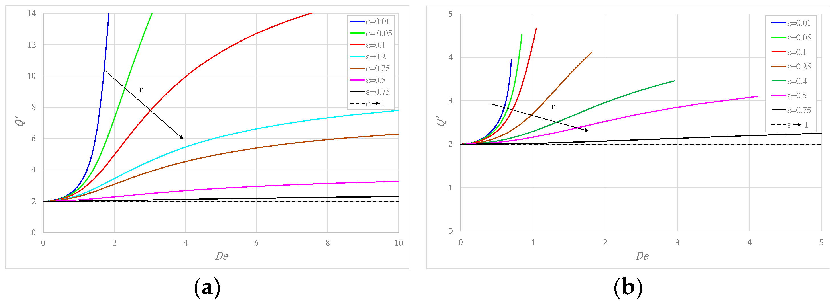
Figure 2a shows for $\beta =0.25$ the behavior of the flow rate per unit width $Q^{\prime }$ as a function of Deborah number $De$ for different values of $\epsilon$: $Q^{\prime }$ initially increases with $De$ and then approaches a constant asymptotic value. Notably, the $De$ increase is physically limited, as eventually the flow regime becomes turbulent for high values of the pressure gradient. At the same time, for an identical value of the pressure gradient, i.e., $De$, an increase in the amount of solvent (larger $\epsilon$) implies a smaller flow rate. This effect, due to a reduction in the shear thinning behavior of the fluid in laminar flow, is more marked for small $\epsilon$ values, while already for $\epsilon \cong 0.5$, the increase is modest with $De$. Figure 2b illustrates the variation of the flow rate $Q^{\prime }$ with $De$ for different and increasing values of $\epsilon$ for $\beta =0.75$; $Q\prime$ initially increases with $De$ as before, but its asymptotic value is not reached (except for $\epsilon$ = 0.75), as with $\beta >0.5$ there is a minimum value of $\epsilon$ to obtain the assigned value of Deborah number as detailed in [14].

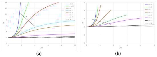
Figure 2. The flow rate versus Deborah number: (a) for $\beta =0.25$; (b) for $\beta =0.75$.

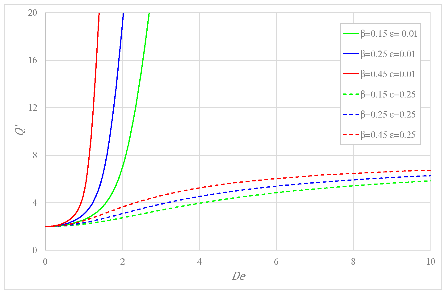
The influence of the mobility factor on the flow rate is described in Figure 3, where one sees that $Q^{\prime }$ is larger for greater mobility $\beta$ and the same $De$ and $\epsilon$; the impact of $\beta$ is decidedly more evident for small $\epsilon$.

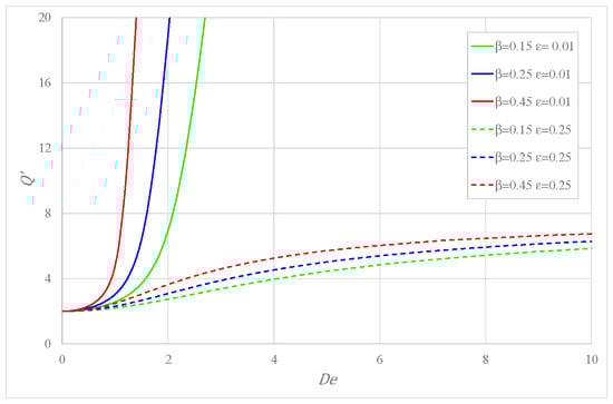
Figure 3. Variation of the flow rate versus Deborah number for some $\beta <0.5$.

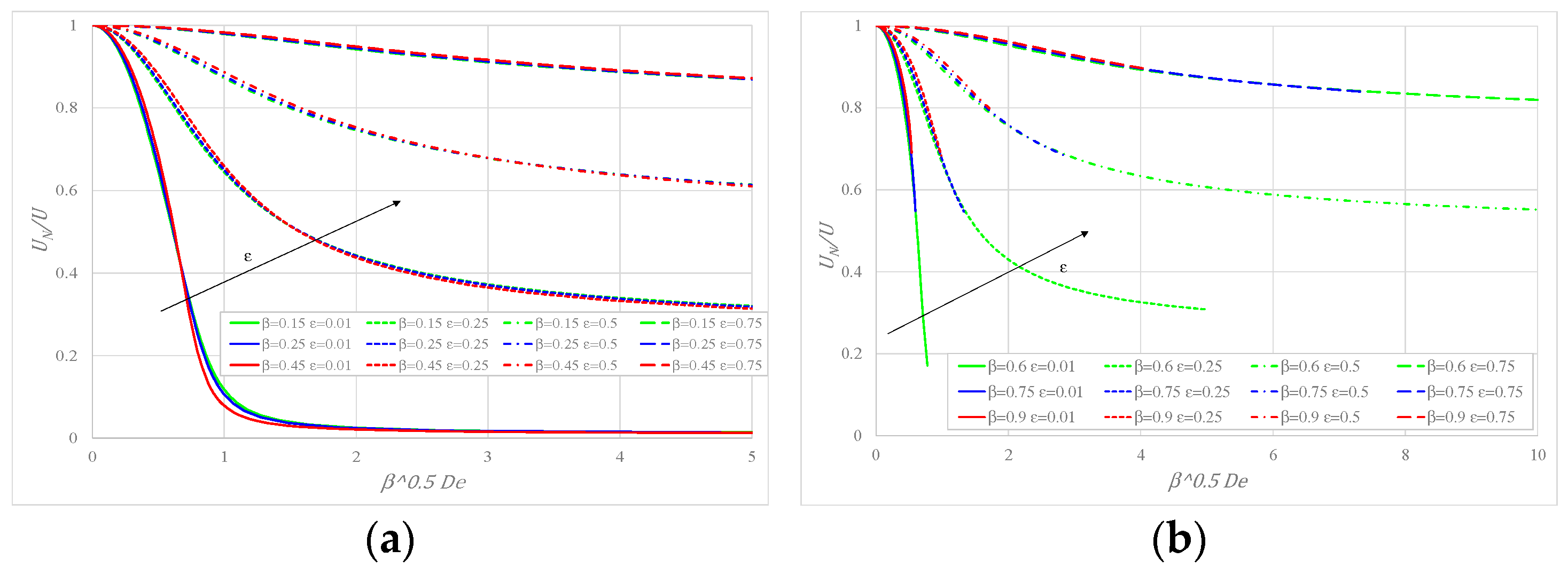
The variation of $U_N/U$ (ratio between the Newtonian and actual mean velocities) with the group $\sqrt{\beta }De$, having $\beta$ and $\epsilon$ as parameters, is shown in Figure 4a for some values of $\beta <0.5$ and in Figure 4b for $\beta >0.5$. In the initial portion of the curves, there is a very rapid decrease of friction due to the shear-thinning behavior of the fluid, which is evident for low values of $\epsilon$; less so as epsilon increases, the reduction being practically absent for $\epsilon =0.75$. For the same value of $\epsilon$, the curves perfectly overlap, showing that, as with other fluids such as PPT and FENE-P (Cruz et. al. [11]), the friction factor depends on $\sqrt{\beta }De$, but not on $\beta$ and $De$ separately.

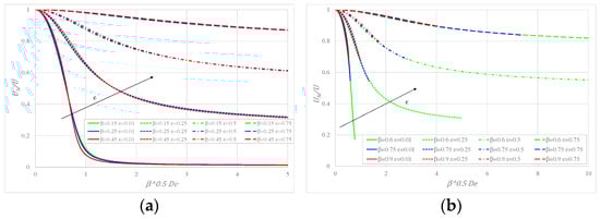
Figure 4. Ratio between the two mean velocities versus elasticity with $\epsilon$ as a parameter: (a) for $\beta =0.25$; (b) for $\beta =0.75$.

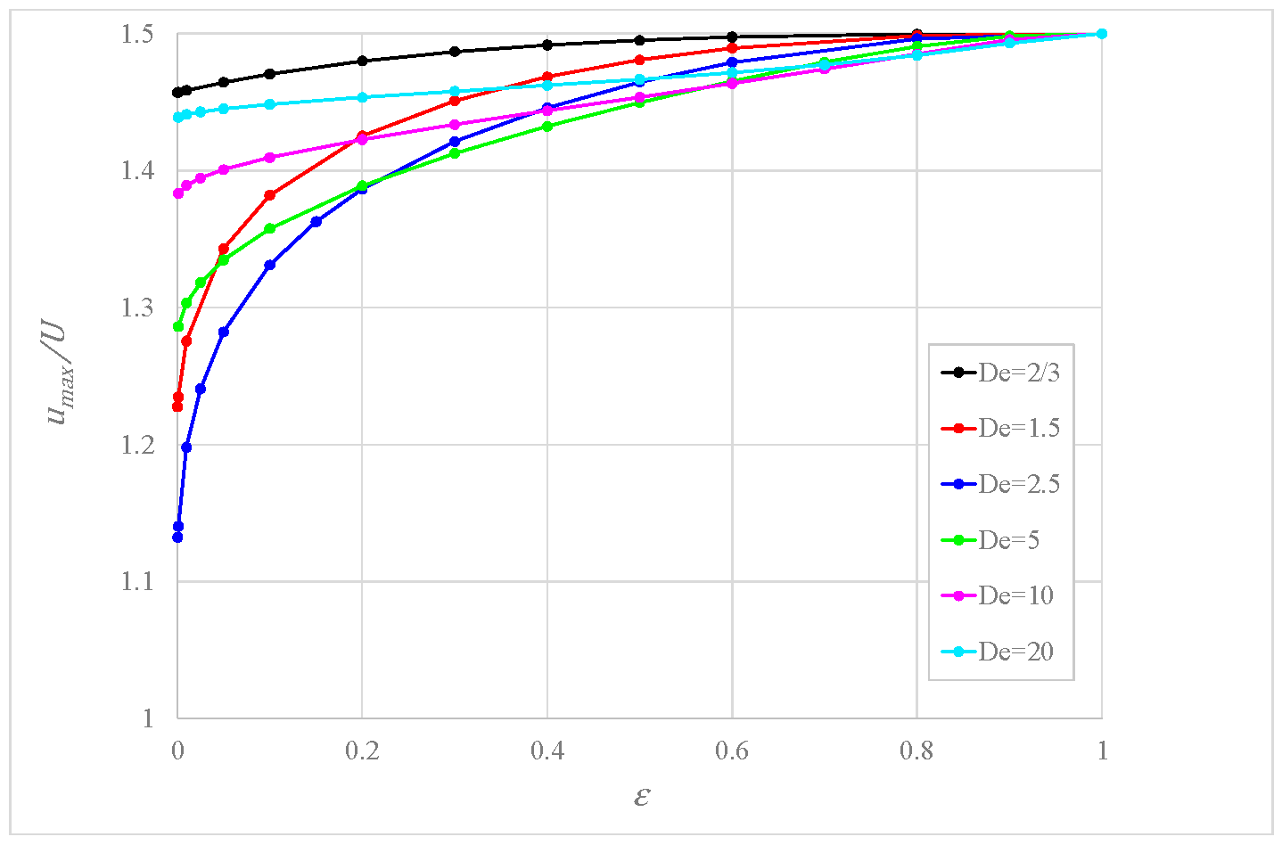
Figure 5 illustrates the ratio $u_{max}/U$ as a function of $\epsilon$ for various $De$ values for fixed $\beta =0.25$. It is seen that $u_{max}/U$, a measure of the flatness of the velocity profile, increases with $\epsilon$, tending to the value 1.5 typical of Newtonian fluids; this means that the velocity profile tends to become parabolic. The dependency on $De$ is not monotonic, but at any rate, the $u_{max}/U$ value is less than 1.5, indicating a velocity profile flatter than the Newtonian one.

Figure 5. Ratio between the maximum velocity and the mean velocity versus $\epsilon$ for some values of $De,$ for $\beta =0.25$.

7. Conclusions

This study investigates the influence of the presence of a Newtonian solvent on the flow of a Giesekus fluid in a plane channel or fracture subject to an assigned pressure gradient. The derivation of the velocity field by first principles yields by analytical integration the flow rate per unit width $Q^{\prime }$ as a function of Deborah number $De$, viscosity ratio $\epsilon$ and dimensionless mobility parameter $\beta$. The key results are as follows:

-

$Q^{\prime }$ increases with $De$ (a proxy of the pressure gradient for a given fluid) and tends to a constant asymptotic value for large $De$, subject to the limitation of laminar flow.

-

For given $De$, smaller flow rates are associated to an increase in the amount of solvent, i.e., larger $\epsilon$. This effect is more marked for small $\epsilon$ values and diminishes for $\epsilon$ in the order of 0.5.

-

$Q^{\prime }$ is decidedly affected by the mobility factor $\beta$ for very small values of $\epsilon$ (a nearly pure shear-thinning fluid), while the impact of $\beta$ is modest for larger $\epsilon$ values.

-

The ratio $U_N/U$ between Newtonian and actual average velocities for a given pressure gradient depends only on the product $\sqrt{\beta }De$.

-

The ratio $u_{max}/U$, expressing the shape of the velocity profile, increases with $\epsilon$ tending to Newtonian behavior for $\epsilon \to 1$ and is affected by the interplay between $De$ and $\beta$.

-

The friction factor depends on $\sqrt{\beta }De$, but not on $\beta$ and $De$ separately, as is the case for other fluids such as PPT and FENE-P [11].

Perspectives for future work are manifold, and include the following: (i) the adoption of more realistic constitutive equations for non-Newtonian flow in fractured rocks, see Lenci et al. [18]; (ii) an extension of the Giesekus free-surface flow case of Tome et al. [19], adding the solvent effect; iii) an extension of the non-isothermal study of Baranovskii [20] to the Giesekus flow with solvent.

References

- Duvarci, O.C.; Yazar, G.; Kokini, J.L.; SAOS, T. MAOS and LAOS behavior of a concentrated suspension of tomato paste and its prediction using the Bird-Carreau (SAOS) and Giesekus models (MAOS-LAOS). J. Food Eng. 2017, 208, 77–88. [Google Scholar] [CrossRef]
- Giesekus, H. A simple constitutive equation for polymer fluids based on the concept of deformation-dependent tensorial mobility. J. Non-Newton. Fluid Mech. 1982, 11, 69–109. [Google Scholar] [CrossRef]
- Giesekus, H. Constitutive equations for polymer fluids based on the concept of configuration-dependent molecular mobility: A generalized mean-configuration model. J. Non-Newton. Fluid Mech. 1985, 17, 349–372. [Google Scholar] [CrossRef]
- Debbaut, G.; Burhin, H. Large amplitude oscillatory shear and Fourier-transform rheology for a high-density polyethylene: Experiments and numerical simulation. J. Rheol. 2002, 46, 1155–1176. [Google Scholar] [CrossRef]
- Calin, A.; Wilhelm, M.; Balan, C. Determination of the non-linear parameter (mobility factor) of the Giesekus constitutive model using LAOS procedure. J. Non-Newton. Fluid Mech. 2010, 165, 1564–1577. [Google Scholar] [CrossRef]
- Rehage, H.; Fuchs, R. Experimental and numerical investigations of the non-linear rheological properties of viscoelastic surfactant solutions: Application and failing of the one-mode Giesekus model. Colloid Polym. Sci. 2015, 293, 3249–3265. [Google Scholar] [CrossRef]
- Yoo, J.Y.; Choi, H.C. On the steady simple shear flows of the one-mode Giesekus fluid. Rheol. Acta 1989, 28, 13–24. [Google Scholar] [CrossRef]
- Schleiniger, G.R.J. Weinacht: Steady Poiseuille flows for a Giesekus fluid. J. Non-Newton. Fluid Mech. 1991, 40, 79–102. [Google Scholar] [CrossRef]
- Daprà, I.G. Scarpi: Couette-Poiseuille flow of the Giesekus model between parallel plates. Rheol. Acta 2009, 48, 117–120. [Google Scholar] [CrossRef]
- Ferrás, L.L.; Nóbrega, J.M.; Pinho, F.T. Analytical solutions for channel flows of Phan-Thien-Tanner and Giesekus fluids under slip. J. Non-Newton. Fluid Mech. 2012, 171–172, 97–105. [Google Scholar] [CrossRef]
- Cruz DO, A.; Pinho, F.; Oliveira, P.J. Analytical solutions for fully developed laminar flow of some viscoelastic liquids with a Newtonian solvent contribution. J. Non-Newton. Fluid Mech. 2005, 132, 28–35. [Google Scholar] [CrossRef]
- de Araujo, M.T.; Furlan, L.; Brandi, A.; Souza, L. A semi-analytical method for channel and pipe flows for the linear Phan-Thien-Tanner fluid model with a solvent contribution. Polymers 2022, 14, 4675. [Google Scholar] [CrossRef] [PubMed]
- da Silva Furlan, L.J.; de Araujo, M.T.; Brandi, A.C.; de Almeida Cruz, D.O.; de Souza, L.F. Different Formulations to Solve Giesekus Model for Flow between Two Parallel Plates. Appl. Sci. 2021, 11, 10115. [Google Scholar] [CrossRef]
- Daprà, I.; Scarpi, G. Analytical solution for channel flow of a Giesekus fluid with non-zero solvent viscosity. J. Non-Newton. Fluid Mech. 2023, 322, 105152. [Google Scholar] [CrossRef]
- Bird, R.B.; Armstrong, R.C.; Hassager, O. Dynamics of Polymeric Liquids; Wiley: New York, NY, USA, 1987. [Google Scholar]
- Deville, M.O.; Gatski, T.B. Mathematical Modelling for Complex Fluids and Flows; Springer: Berlin/Heidelberg, Germany, 2012. [Google Scholar]
- Giesekus, H. Die rheologische Zustandsgleichung elasto-viskoser Flüssigkeiten—Insbesondere von Weissenberg-Flüssigkeiten—Für allgemeine und stationäre Fließvorgänge. J. Appl. Math. Mech. Z. Fur Angew. Math. Mech. 1962, 42, 32–61. [Google Scholar] [CrossRef]
- Lenci, A.; Mehéust, Y.; Putti, M.; Di Federico, V. Monte Carlo simulations of shear-thinning flow in geological fractures. Water Resour. Res. 2022, 58, e2022WR032024. [Google Scholar] [CrossRef]
- Tome, M.F.; Araujo, M.T.; Evans, J.D.; McKee, S. Numerical solution of the Giesekus model for incompressible free surface flows without solvent viscosity. J. Non-Newton. Fluid Mech. 2018, 263, 104–119. [Google Scholar] [CrossRef]
- Baranovskii, E.S. Exact Solutions for Non-Isothermal Flows of Second Grade Fluid between Parallel Plates. Nanomaterials 2023, 13, 1409. [Google Scholar] [CrossRef]
Disclaimer/Publisher’s Note: The statements, opinions and data contained in all publications are solely those of the individual author(s) and contributor(s) and not of MDPI and/or the editor(s). MDPI and/or the editor(s) disclaim responsibility for any injury to people or property resulting from any ideas, methods, instructions or products referred to in the content. |
© 2024 by the authors. Licensee MDPI, Basel, Switzerland. This article is an open access article distributed under the terms and conditions of the Creative Commons Attribution (CC BY) license (https://creativecommons.org/licenses/by/4.0/).