Article

A Preliminary Investigation of a Single Shock Impact on Italian Mortality Rates Using STMF Data: A Case Study of COVID-19

by
Maria Francesca Carfora
* and
Albina Orlando
*
Istituto per le Applicazioni del Calcolo “Mauro Picone”, Consiglio Nazionale delle Ricerche, Via P. Castellino, 111, 80131 Naples, Italy
*
Authors to whom correspondence should be addressed.
Data 2023, 8(6), 107; https://doi.org/10.3390/data8060107
Submission received: 2 May 2023 / Revised: 9 June 2023 / Accepted: 10 June 2023 / Published: 13 June 2023

Abstract

:
Mortality shocks, such as pandemics, threaten the consolidated longevity improvements, confirmed in the last decades for the majority of western countries. Indeed, just before the COVID-19 pandemic, mortality was falling for all ages, with a different behavior according to different ages and countries. It is indubitable that the changes in the population longevity induced by shock events, even transitory ones, affecting demographic projections, have financial implications in public spending as well as in pension plans and life insurance. The Short Term Mortality Fluctuations (STMF) data series, providing data of all-cause mortality fluctuations by week within each calendar year for 38 countries worldwide, offers a powerful tool to timely analyze the effects of the mortality shock caused by the COVID-19 pandemic on Italian mortality rates. This dataset, recently made available as a new component of the Human Mortality Database, is described and techniques for the integration of its data with the historical mortality time series are proposed. Then, to forecast mortality rates, the well-known stochastic mortality model proposed by Lee and Carter in 1992 is first considered, to be consistent with the internal processing of the Human Mortality Database, where exposures are estimated by the Lee–Carter model; empirical results are discussed both on the estimation of the model coefficients and on the forecast of the mortality rates. In detail, we show how the integration of the yearly aggregated STMF data in the HMD database allows the Lee–Carter model to capture the complex evolution of the Italian mortality rates, including the higher lethality for males and older people, in the years that follow a large shock event such as the COVID-19 pandemic. Finally, we discuss some key points concerning the improvement of existing models to take into account mortality shocks and evaluate their impact on future mortality dynamics.

1. Introduction

According to the World Health Organization (WHO), a pandemic can start when three conditions occur: the emergence of a disease is new to the population, the agent infects humans causing serious disease, the agent spreads easily and sustainably among humans [1]. Pandemics can threaten millions of lives, damage societies, and take down economies. The full death toll due to the COVID-19 pandemic was approximately of 14.9 million (range from 13.3 million to 16.6 million) [2]. These estimates refer to the “excess mortality” between January 2020 and 31 December 2021 which is assessed as the difference between the number of deaths that have occurred and the number that would be expected in the absence of the pandemic, relying on data from earlier years. Excess mortality includes deaths due to the COVID-19 disease and the ones due to the pandemics impact on health systems and society. Most of the excess deaths (84%) are concentrated in South-East Asia, Europe, and the Americas.
The mortality shock due to a pandemic can seriously affect life insurance contracts, depending on the insurance portfolio structure. As regards the effects of COVID-19 pandemic on Italian insurance market, according to the Italian National Association of Insurance Companies (ANIA) [3], premiums from domestic and foreign business, direct and indirect, gross of reinsurance, contracted by 3.9% in 2020, after two consecutive years of growth (+3.1% in 2018 and +3.9% in 2019). The overall contraction reflects the trend of both the life sector, whose premiums went down by 4.5% (+3.8% in 2019), and the non-life sector, where premiums dropped by 2.0% after 4.2% growth the previous year. In the life sector the technical account result remained positive at €3.4 billion, but down from €6.4 billion the previous year, and the ratio to premiums slumped from 6.0% to 3.3%. In general, increased mortality could cause losses for which the company may not be sufficiently prepared. Indeed, a relevant issue is the obligation of insurers to comply with the Solvency II Regulation, meaning that they must set aside a mortality risk capital to cover losses due to a permanent 15% increase in mortality rates. Even if the consequences of a pandemic should not be so extreme in terms of long-term changes of mortality rates, it is likely that even if transitory mortality jumps of this size may occur, the financial consequences could be non-negligible. Several contributions to the recent actuarial literature deal with the impact of COVID-19 pandemic on life insurance domain [4,5,6]. The need for taking into account the COVID-19 effects in modeling mortality is essential for insurance companies regadring valuations, reserving decisions or solvency capital calculations. To this aim, adjusting stochastic mortality models is strongly required. To be more specific, mortality shocks, such as pandemics, threaten the consolidated longevity improvements, confirmed in the last decades for the majority of western countries. Just before the COVID-19 pandemic, mortality was falling at all ages, with a different behavior according to different ages and countries. In this context, the changes in the population longevity induced by shock events, even transitory ones, affect demographic projections, and have financial implications in public spending as well as in pension plans and life insurance. In the light of these considerations, our aim is to analyze the effects of the mortality shock caused by the COVID-19 pandemic on Italian mortality rates. We adopt an actuarial perspective and, for this reason, we refer to the stochastic mortality models used in this domain. We believe this study could be the basis for quantifying the potential impact of mortality shocks on the main life insurance contracts.
The COVID-19 pandemic is indeed a remarkable case study, providing plenty of data to: investigate whether a single shock had a notable impact on mortality rates; recalibrate well-established mortality models; estimate how mortality jumps influence uncertainty in their forecasts; discuss and evaluate their potential impact on insurance valuation applications. The most used indicator for quantifying the effect of a pandemic is the excess mortality, defined as the number of deaths observed during the pandemic above a baseline of recent trends (among the huge literature, see the very recent studies by Refs. [7,8,9] for COVID-19-related studies). Data on all cause mortality are considered by national Statistic Offices as more reliable indicators with respect to data registered as pandemic related mortality “because they are less sensitive to coding errors, competing risks, and the potential for misclassification in designating the cause of deaths” [10]. Another useful indicator for population health is life expectancy at birth, defined as the average life length in years of a hypothetical cohort assumed to experience, from birth through death, the mortality rates observed in a given period. Changes in life expectancy have been used in the recent literature [10,11,12] to provide cross-national comparison of the population-level COVID impact, because they are not influenced by variations in populations size and age structure across countries. Other indicators, such as YLL, Years-of-Life-Lost, have also been considered [10] because they can provide a finer estimate of premature mortality, by weighting differently deaths occurring at younger and older ages. Their contribution could be useful in further refining pandemic-related demographic studies.
Previous experience of mortality shocks due to pandemics, such as the ones observed during the most severe seasonal flu epidemics, can furnish useful lessons about volatility spikes in deaths. However, there are also significant differences. First, the severity of the shock: as observed in recent studies on life expectancy changes after a pandemic [11], the worst recent flu epidemics (2014–2015) produced a shock in most high-income countries, causing severe drops in life expectancy, whose largest value (observed in Italy) was about half a year lost for both males and females. The current estimates for 2020 for a panel of more than 20 countries is a loss in life expectancy of more than a year. Second, cross-age impact: as many studies confirm (see Ref. [7] and references therein), COVID-19 death rates are roughly proportional to all-cause mortality, while in past epidemics spikes in deaths tended to be smaller for younger ages and were more significant in older population. Third, long-range consequences: lockdowns and similar measures lead to indirect consequences of the pandemics, such as delays in other medical diagnoses and therapies, recession of the economy, increase in self-isolation, alcohol and drug consumption, all resulting in long-term reduction of life expectancy. On the other side, durable changes in social behavior, such as masks wearing and avoiding overcrowded environments, just to mention a few, could lead to reduced mortality in certain population groups. Even if researchers are still unable to quantify the impact of these indirect effects on mortality changes, long-term modifications of the mortality curve should be considered in the next years.
The aim of this paper is to investigate the impact of the mortality shock due to the COVID-19 pandemic on Italian mortality rates. The reference dataset is the Human Mortality Database (HMD, [13]) as combined with the Short Term Mortality Fluctuations (STMF) data series, released by the HMD team in 2020. The STMF is a new component of the HMD providing data of all-cause mortality fluctuations by week within each calendar year. After merging these two datasets, we model mortality by means of the well-known stochastic model proposed by Lee and Carter in 1992. In the present work we choose to simply rely on the Lee–Carter model for consistency with the internal processing of the Human Mortality Dataset: although alternative models have been proposed to improve some drawbacks of this simple model (see [14], for a review), they are not designed to include shock effects. Instead, we suggest some generalizations of the Lee–Carter model, proposed in the recent literature [15], that are specifically aimed at modeling mortality shocks in view of the improvements they can bring. Empirical results are discussed both on the estimation of the model coefficients and on the forecast of the mortality rates.

2. Materials and Methods

2.1. Demographic Data

The Human Mortality Database (HMD) is one of the most used and cited data resources in demography. It was launched in May 2002 to provide detailed and highly reliable mortality and population estimates to those interested in human longevity: researchers, students, journalists, and policy analysts. The HMD follows open data principles; financial and logistical support are provided by sponsoring institutions, such as the Department of Demography at the University of California, Berkeley (UCB), the Max Planck Institute for Demographic Research (MPIDR), and the French Institute for Demographic Studies (INED). Nowadays, HMD contains original calculations of death rates and life tables for 41 countries and areas and an additional 8 sub-populations, as well as the raw data (death counts, census counts, birth counts, and population estimates from various sources) used in constructing those tables. Due to data quality requirements, the database is limited to populations where death registration and census data are virtually complete, so that the countries and areas included are relatively wealthy and highly industrialized. A companion project (Human Lifetable Database, HLD) includes life tables constructed by other institutions and mortality estimates for some countries (both developed and developing ones) that could not be included in the HMD.
The complete data series includes collected and estimated data. Period data are indexed by calendar year, whereas cohort data (if available) are indexed by year of birth. All files are organized by sex, age, and time. The collected data comprise: live birth counts (annual, by sex); death counts (annual, at the finest level of age detail available, as reported below, by sex), in the following denoted by D t i m e ( a g e ) ; population size on 1 January (annual estimates either obtained from another source or from census data plus birth and death counts), in the following denoted by P t i m e ( a g e ) . Population size is given for both one-year and five-year age groups (specifically: ages 0, 1–4, 5–9, 10–14, …, 105–109, with an open age interval for 110+).
The estimated data comprise: population exposed to risk of death (during a given age-time interval, based on annual population estimates), denoted by E t i m e ( a g e ) ; death rates (the death count for a given age-time interval divided by an estimate of the exposure-to-risk in the same interval); life tables (life expectancies and other indicators of mortality and longevity). Deaths, exposure-to-risk, death rates, and life tables are given in several formats of age and time: 1 × 1 (by age and year); 1 × 5 (by age and 5-year time interval); 5 × 1 (by 5-year age group and year); and coarser grouping such as 5 × 5, 1 × 10, 5 × 10. At the finest level of detail, available data include, separately for male and female population, the exposures E t ( x ) , estimated as the population of age x at 30 June, year t, and the death counts D t ( x ) , expressing deaths in year t of persons of age x, from which one can obtain the central mortality rate at age x in year t as m x t = D t ( x ) / E t ( x ) .
The Short-term Mortality Fluctuations (STMF) data series [16,17] are a new component of the Human Mortality Database (HMD). These series are established to provide data for scientific analysis of all-cause mortality fluctuations by week within each calendar year. An interactive graphical interface, the STMF online visualization tool, publicly available at https://mpidr.shinyapps.io/stmortality/ (accessed on 9 June 2023), is also provided to quickly obtain an overview of the excess weekly mortality in a specific country and year. The decision to add this new resource to the HMD was triggered by the COVID-19 pandemic. An additional motivation for this HMD extension was the increasing importance of short-term or seasonal mortality fluctuations that are driven by temporary hazards such as influenza epidemics, temperature extremes, as well as man-made or natural disasters.
The relative importance of short-term excess mortality increases in the context of a general mortality decline. It is also important also these particular problems tend to disproportionally affect vulnerable population groups such as the elderly.
It is worth remarking the main characteristics of STMF data:
  • They only cover a subset (38 out of the 48) of countries included in the HMD; moreover, the length of the country-specific data series varies: the longest time series (Finland) starts in 1990, the shorter ones (Chile, Greece, and Germany) in 2016. Most of the country series (23 out of the 38) begin in 2000. The series are neither smoothed nor adjusted for data quality problems such as death undercounts. Deaths are generally collected by date of occurrence, apart from UK data (England, Scotland, Wales, Northern Ireland), which are collected by date of registration;
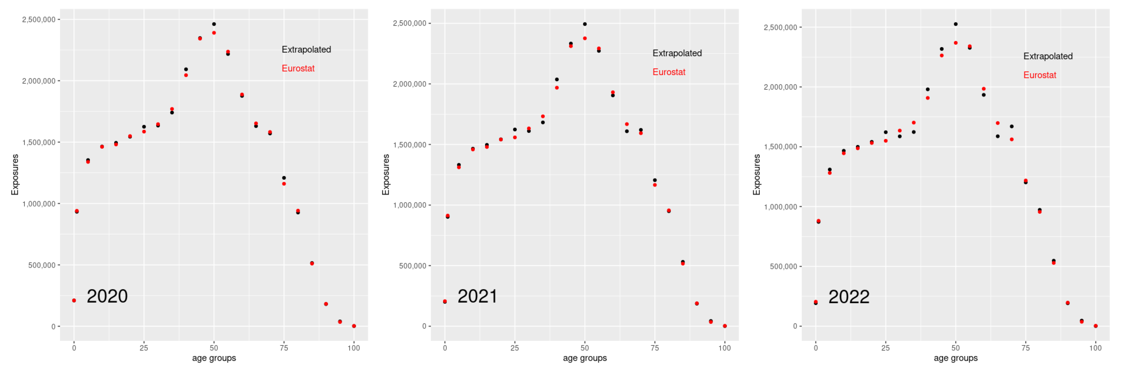
  • Weekly death rates are obtained from collected weekly death counts (generally registered by sex and age) and estimated annual population exposures; For the more recent years, when annual data are not yet available, the exposures are estimated after extrapolating annual death rates by fitting a Lee–Carter model to the HMD data; in this case, a relatively short reference period is chosen to appreciate the most recent changes in mortality;
  • The original data for each country are split or grouped in standard age groups in order to be consistent across countries; however, raw data at country level with finer age grouping (5 years) are often available; for example, as reported below, Italian raw data contain death counts for all-cause mortality cross-classified by week, year, sex, 5-years age interval.
Italian raw data contain weekly death counts D y w , s e x ( x , x + a ) for each year y from 2011 to 2022 (plus the first 4 weeks of 2023 at the present time). Data are sex-specific (male, female, and total population) and reported for age groups 0, 1–4, 5–9, 10–14, …, 95–99, 100+ Weekly rates are obtained from collected weekly death counts and estimated (or forecasted) annual population exposures. As an example, we obtain the weekly mortality rate for male population in the age range ( x , x + a ) for week w and year y as
m y w , m a l e s ( x , x + a ) = D y w , m a l e s ( x , x + a ) E y m a l e s ( x , x + a ) / 52 .

2.2. Data Processing

As thoroughly discussed in [18], excess mortality estimates are quite sensitive to processing choices, such as the chosen mortality index (death counts or rates), the reference period, and the time unit of the death series. These sources of variation can produce significant differences in the estimates of excess mortality provided by different authors, as seen for the COVID-19 pandemic. Inconsistencies in such estimates, also in case of cross-country comparisons, can affect policy decisions and reduce the efficiency of measures. Based on these considerations, researchers should be very precise in describing all the steps of their data processing, to allow a fair use of their results. This is the reason why we describe here in detail the procedure we adopted for processing mortality data, starting from the merging of the two considered dataset. STMF Italian data are weekly death counts for males/females, grouped in 5-years age groups up to age 100+, while Italian data in the HMD dataset also include 5-years age grouped data from 0 to 110+ in the time period 1872–2019. Then we extracted from HMD the Italian death counts, rates, and exposures and grouped data for the older ages (100+); we also aggregated STMF weekly deaths for each age group to obtain estimates of the yearly death counts for 2020, 2021, and 2022. These counts, appended to the HMD data, provided us with a complete series of yearly death counts. To obtain the yearly death rates for 2020 to 2022, we also needed to estimate the corresponding exposures. Following similar studies [9], we extrapolated them linearly for each age and sex from the last five exposures (2015 to 2019) in HMD data; since year 2015 presents a peak value in the observed exposures, this choice for the time window is the most appropriate to guarantee coherence with the observed slightly decreasing trend in the last years. However, to assess the accuracy of such an extrapolation, we compared the estimated exposures to the ones we derived from Eurostat [19] data; specifically, we retrieved the death counts for each age and sex for the years 2020 to 2022 along with the corresponding population values and processed them to obtain an independent estimate for the exposures. Figure 1 provides a graphical comparison of these estimates, confirming a very good agreement between them and so assessing the reliability of the extrapolation procedure.
Figure 2 shows the yearly death rates for the years 2011–2022, separately for the male and female populations, as retrieved from the combined dataset HMD + STMF. Rates for the more recent years, plotted in violet, are obtained from the aggregation of STMF data; while affected by a higher roughness, they carry valuable information on the sensible increase in death rates: for several age groups, and more evidently in older ages, the violet curves are not the lowest ones, as expected in the framework of decreasing mortality that characterized Italy in the recent past. On the contrary, they confirm a sharp increase in mortality rates, clearly visible in the right part of each plot.

2.3. Basic Mortality Model

Lee and Carter [20] proposed the following principal component model to forecast demographic data
log m x t = a x + b x k t + ϵ x t , x = 1 , h ; t = t 1 , t n
where m x t = D x t / E x t is the observed mortality rate at age x in year t; its logarithm is modeled as an average age profile of the rate over the years ( a x ) modified by the combined effects of time t at each age ( b x ) and mortality changes over time ( k t ); the residual term ϵ x t represents the age and time specific trends not fully captured by the model. In the original version, parameters were estimated by a two-stage process: after estimating the mean as
a ^ x = 1 t n t 1 t = t 1 t n log m x t ;
a Singular Value Decomposition of
log m x t a ^ x = i = 1 min ( n , m ) s i u x i v t i
leads to the estimates
k ^ t S V D = s 1 v t 1 ; b ^ x S V D = u x 1 ;
additional constraints guarantee the identifiability of the model:
x b ^ x = 1 and t k ^ t = 0 .
Alternative frameworks have been proposed over the years in order to improve some drawbacks of the Lee–Carter model. We already compared, in a previous work [14], the original model with several modified models for mortality rates, including generalized nonlinear models where the error is assumed as Binomial or Poisson distributed and where two or more terms are retained in the truncated SVD approximation. Other extensions introduce cohort (year of birth) parameters to account for the significant impact of such effects, while functional demographic models such as the regularized SVD extend the principal components approach by adopting a functional data paradigm. Our results in the cited work showed that functional models slightly improve on the basic Lee–Carter performance and that cohort effect should be considered, even in a post-processing correction. However, in the present work, we choose to simply rely on the Lee–Carter model to be consistent with the internal processing of the Human Mortality Dataset, where exposures are estimated, when needed, by Lee–Carter. As far as forecasts are concerned, in the basic model by Lee and Carter they are obtained by modeling the time series for the period effect k t as a random walk with drift; some generalizations also consider ARIMA models for k t to generate mortality forecasts.

2.4. Models including Mortality Jumps

In the last years, some authors [15,21,22] have proposed refinements of the Lee–Carter model to include mortality jumps: short-term jump effects are represented by adding a multiplicative term N t J x , t to the mortality rate, where N t is a jump count (Bernoulli) variable and J x , t describes the effect of a jump in mortality on year t on a group aged x. The model can be written as
log m x t = a x + b x k t + N t J x , t + ϵ x t
and different assumptions on correlation between age groups lead to different specifications of the jump vector J t , which is generally modeled by a multivariate Gaussian variable. In such a modeling choice, k t is assumed to be free of jumps and follows a random walk with trend as in the basic Lee–Carter model. Estimation of the model parameters is quite cumbersome; it is generally performed via an iterative maximization of the likelihood function.

3. Results

To estimate the coefficients of the Lee–Carter model on the HMD data, the choice of the reference period is quite relevant: a longer time series can guarantee a smoother fit, but this choice can also result in underestimation of recent trends, such as the more pronounced longevity improvements observed in many countries. On the other side, very short time series could excessively increase the weight of specific past shocks (such as the peaks corresponding to the severe influenza seasons of 2013 and 2015) on the model estimation. The more relevant and recent literature reflects both approaches: while some authors used long series, starting from 1988 [8] or 1991 [9], others considered shorter ones, starting from 2005 [10] or even 2015 [12]. Then, to temper the requirements of smoothness of the estimate and major relevance of recent years, we decided to consider Italian mortality data from HMD for the time period 2000–2019 (the last available year); Lee–Carter estimates of the model coefficients have been obtained in R software environment, package demography [23], and are shown in Figure 3. In the following we denote this model by LC19. These model coefficients should be compared to the ones obtained by estimating a Lee–Carter model on the full dataset, comprising HMD data along with the yearly aggregated STMF data for the years 2020 to 2022. This model will be denoted by LC22; its coefficients are shown in Figure 4.
As expected, the coefficient a x , describing the general mortality trend across ages (shown in the left panel of both Figure 3 and Figure 4), is essentially unaltered by the additional information over the last three years; the pandemic years start showing their effects on mortality rates only in the first order correction b x (shown in the central panel of the same figures), where modifications on all the three curves appear. While for the male population these modifications affect the older ages, starting at about age 60, the female population is affected also at young ages. The changes in both curves are far more pronounced for the older ages (aged 80 and more). However, the most significant changes concern the period effect k t . Indeed, as proven in Ref. [9], the main effect of a mortality shock in year t is a jump in the period effect k t for that year, while the other model parameters are less affected. A visual comparison of the right panels of Figure 3 and Figure 4 confirms that the inclusion of data from the STMF dataset allows to appreciate quite a large upward jump in the period effect k t for year 2020 and an initial bounce back for year 2021, confirmed in 2022. Forecast death rates are strongly affected by these differences in calibrated parameters, especially when the shock year is the last one in the reference period for forecasts, due to the very nature of the adopted model (random walk with trend or ARIMA). Just to show an example, the following Figure 5 and Figure 6 report the forecasts for the period effect k t in the next three years based on the two considered models, LC19 and LC22, respectively. While the former, having no information on the pandemic shock, provides a forecast of the continuously decreasing period effect in the years from 2020 to 2022, the latter, relying on information on both the shock year 2020 and the less severe 2021 and 2022, shows in the forecast value for k t in the following years a partial recovering from the shock event. These values, on the other side, are accompanied by wider confidence intervals, because of the higher fluctuations affecting the more recent years. However, it should be noted that the Lee–Carter model shows all of its limitations in presence of such a severe shock: a more sophisticated model, able to separate the smooth component of the period effect from the jump term, would be more effective in capturing the actual trend in mortality rates. It is also worth noting that the curves in Figure 5 and Figure 6, while showing comparable behavior, differ in scale. This is a consequence of the estimation procedure, which retrieves the values for b x and k t up to a scale factor (the scaling singular value in the SVD decomposition).

4. Conclusions

After a very long period of improvements in life expectancy in almost all countries (approximately since the end of World War II), the COVID-19 pandemic led to significant shocks in the mortality rates dynamics, starting from March 2020. These shocks result in a general increase of mortality rates, with significant differences in terms of timing and severity in different countries. However, even restricting the analysis to a single nation, as we did for Italy in this study, the impacts of the pandemic on mortality rates have been highly heterogeneous across sexes and age groups, since the observed lethality of COVID-19 was higher for males and older people; investigating such a situation requires more timely data as well as improved mortality models to be able to capture the complex dynamics following a large shock event such as the COVID-19 pandemic. In this perspective, the availability of STMF data and their integration in the HMD dataset to represent the recent years trend allowed us to correctly reproduce the large increase in mortality rates that occurred in 2020 and the partial bounce back in the following two years.
In conclusion, these first empirical results confirm that STMF data are a new and valuable resource to timely appreciate changes in mortality that occur as consequences of shock events, but they also highlight some drawbacks of these data to be further considered. First, due to their age coarseness and their roughness, they require suitable refining and smoothing procedures in preprocessing. Moreover, being a new tool, they need further validation; their harmonization with other datasets (HMD, but also Eurostat) is not yet complete. Apart from these caveats, we have proved that mortality data from the combined dataset (HMD + STMF) allow to capture a jump in mortality rates, mainly due to the period effect k t ; this jump is driven by older ages rates deterioration, but it can lead to overestimation of mortality, especially at younger ages. This is because forecasts based on a shock event in the last time period (as captured by STMF data) can be excessively pessimistic. Again, a more accurate model, explicitly including jump terms, could be very useful to correctly describe mortality dynamics; further studies investigating this approach would bring a very valuable contribution to the field.

5. Perspectives for Future Research

Assessing how much a mortality model changes in response to new calibration data, and specifically in response to a mortality shock, is a key point in applications. Indeed, two different question arise: how to recalibrate a given mortality model in case of past shock events? Additionally, how to modify the model to allow for further occurrence of shocks? To adjust an existing model for an observed jump in mortality, there are several possibilities: data referring to shock years can be included as regular data points or they can be treated as outliers, so to remove or at least mitigate their influence on model estimates and forecasts. Again, more general ARIMA models can be considered to predict the period effect time series more robustly. To account for possible future shocks, deeper modifications should be considered, for example by introducing in the modeling of period effects regime switching or jump processes, or even mixture models borrowed from extreme value theory. All these options should be assessed and their estimates and forecasts compared in the context of specific applications as more data become available in the next years.
Another key issue concerns the effects of mortality shocks on life insurance products. Mortality shocks can seriously affect life insurance domain, depending on the portfolio structure. As regards longevity benefits, they are paid if the insured is alive at a certain fixed age. The continuing trend of increasing life expectancy in the past decade has led insurance companies to front and manage the so-called “longevity risk”. It is the potential risk attached to the increasing life expectancy of policyholders, which can result in higher than expected payouts for insurance companies. Further increase in mortality would be profitable to the insurer for these policies. On the other hand, death benefits are paid as a lump sum to beneficiary if the insured dies. Referring to these policies, increased mortality could cause losses to the insurer as the provisions and rates have been calculated according to a lower mortality, leading to a difficulty in covering the claims. The total impact is either loss or profit, depending on the portfolio structure and it could imply that insurers may not fulfill the solvency requirements and therefore would need new capital to continue their business.
Basing on these considerations, the perspective of future work includes estimating the impact of COVID-19 pandemic on the actuarial present values of life insurance contracts with survival benefits, with death benefits and mixed life insurance policies providing both survival and death benefits. In particular, we could compare the results obtained by means of each considered LC model (LC19 and LC22). In order to focus on mortality shocks, at a first stage, a constant discount factor could be fixed. As regards the prediction uncertainty, the interval bounds of forecasted mortality rates could be inserted in the valuation formulae. Some authors [9] propose this approach by estimating the present values of 30-year annuity for a person aged 65 and a 30-year life insurance contract for a person aged 35 at the beginning of 2021 and found, as expected, a drop in annuity values and an increase in life insurance policies (about 29% for Italian males), along with a significant increase in prediction uncertainty. In our opinion, the main issues for this approach concern the length of the prediction interval and the sensitivity of the forecast to the distance from the shock year, which could lead to unreliable results. A reliable estimation procedure would require further recalibrations in the next few years, as more and more new data will be published, to assess the adjustment of the mortality curve towards its pre-pandemic trend.

Author Contributions

Conceptualization, M.F.C. and A.O.; Data curation, M.F.C.; Investigation, A.O.; Methodology, M.F.C. and A.O.; Writing—original draft, M.F.C. and A.O.; Writing—review and editing, M.F.C. and A.O. All authors have read and agreed to the published version of the manuscript.

Funding

This research was partially funded by the H2020-ICT-48 TAILOR Network (GA 952215) and by project SERICS (PE00000014) under the MUR National Recovery and Resilience Plan funded by the European Union—NextGenerationEU.

Institutional Review Board Statement

Not applicable.

Informed Consent Statement

Not applicable.

Data Availability Statement

All data are publicly available through Human Mortality Database and Eurostat websites.

Conflicts of Interest

The authors declare no conflict of interest.

References

  1. Broekhoven, H.; Alm, E.; Tuominen, T.; Hellman, A.; Dziworski, W. Actuarial Reflections on Pandemic Risk and Its Consequences. 2006. Available online: https://actuary.eu/documents/pandemics_web.pdf (accessed on 9 June 2023).
  2. World Health Organization. 14.9 Million Excess Deaths Associated with the COVID-19 Pandemic in 2020 and 2021. 2022. Available online: who.int/news/item/05-05-2022-14.9-million-excess-deaths-were-associated-with-the-covid-19-pandemic-in-2020-and-2021 (accessed on 9 June 2023).
  3. Italian Insurance in 2020–2021. Annual Report of the Italian National Association of Insurance Companies. 2021. Available online: https://www.ania.it/pubblicazioni/-/categories/53731 (accessed on 9 June 2023).
  4. Carannante, M.; D’Amato, V.; Haberman, S. COVID-19 accelerated mortality shocks and the impact on life insurance: The Italian situation. Ann. Actuar. Sci. 2022, 16, 478–497. [Google Scholar] [CrossRef]
  5. Harryz, T.F.; Yelowitz, A.; Courtemanche, C. Did COVID-19 change life insurance offerings? J. Risk Insur. 2021, 88, 831–861. [Google Scholar] [CrossRef] [PubMed]
  6. Zhang, X.; Liao, P.; Chen, X. The negative impact of COVID-19 on life insurers. Front. Public Health Health Econ. Sect. 2021, 9, 756977. [Google Scholar] [CrossRef] [PubMed]
  7. Cairns, A.J.G.; Blake, D.P.; Kessler, A.; Kessler, M. The Impact of COVID-19 on Future Higher-Age Mortality; Technical Report; Pensions Institute: London, UK, 2020. [Google Scholar] [CrossRef]
  8. Robben, J.; Antonio, K.; Devriendt, S. Assessing the Impact of the COVID-19 Shock on a Stochastic Multi-Population Mortality Model. Risks 2022, 10, 26. [Google Scholar] [CrossRef]
  9. Schnürch, S.; Kleinow, T.; Korn, R.; Wagner, A. The impact of mortality shocks on modelling and insurance valuation as exemplified by COVID-19. Ann. Actuar. Sci. 2022, 16, 498–526. [Google Scholar] [CrossRef]
  10. Islam, N.; Jdanov, D.; Shkolnikov, V.; Khunti, K.; Kawachi, I.; White, M.; Lewington, S.; Lacey, B. Effects of COVID-19 pandemic on life expectancy and premature mortality in 2020: Time series analysis in 37 countries. Br. Med. J. 2021, 375, e066768. [Google Scholar] [CrossRef] [PubMed]
  11. Aburto, J.M.; Schöley, J.; Kashnitsky, I.; Zhang, L.; Rahal, C.; Missov, T.I.; Mills, M.C.; Dowd, J.B.; Kashyap, R. Quantifying impacts of the COVID-19 pandemic through life-expectancy losses: A population-level study of 29 countries. Int. J. Epidemiol. 2021, 51, 63–74. [Google Scholar] [CrossRef] [PubMed]
  12. Schöley, J.; Aburto, J.M.; Kashnitsky, I.; Kniffka, M.S.; Zhang, L.; Jaadla, H.; Dowd, J.B.; Kashyap, R. Life expectancy changes since COVID-19. Nat. Hum. Behav. 2022, 6, 1649–1659. [Google Scholar] [CrossRef] [PubMed]
  13. Human Mortality Database. Max Planck Institute for Demographic Research (Germany), University of California, Berkeley (USA), and French Institute for Demographic Studies (France). 2023. Available online: www.mortality.org (accessed on 22 March 2023).
  14. Carfora, M.; Cutillo, L.; Orlando, A. A quantitative comparison of stochastic mortality models on Italian population data. Comput. Stat. Data Anal. 2017, 112, 198–214. [Google Scholar] [CrossRef]
  15. Liu, Y.; Li, J.S.H. The age pattern of transitory mortality jumps and its impact on the pricing of catastrophic mortality bonds. Insur. Math. Econ. 2015, 64, 135–150. [Google Scholar] [CrossRef]
  16. Jdanov, D.; Galarza, A.; Shkolnikov, V.; Jasilionis, D.; Németh, L.; Leon, D.; Boe, C.; Barbieri, M. The short-term mortality fluctuation data series, monitoring mortality shocks across time and space. Sci. Data 2021, 8, 235. [Google Scholar] [CrossRef] [PubMed]
  17. Németh, L.; Jdanov, D.; Shkolnikov, V. An open-sourced, web-based application to analyze weekly excess mortality based on the Short-term Mortality Fluctuations data series. PLoS ONE 2021, 16, e0246663. [Google Scholar] [CrossRef] [PubMed]
  18. Nepomuceno, M.R.; Klimkin, I.; Jdanov, D.A.; Alustiza-Galarza, A.; Shkolnikov, V.M. Sensitivity Analysis of Excess Mortality due to the COVID-19 Pandemic. Popul. Dev. Rev. 2022, 48, 279–302. [Google Scholar] [CrossRef] [PubMed]
  19. Eurostat Database. 2023. Available online: https://ec.europa.eu/eurostat/web/main/data (accessed on 13 April 2023).
  20. Lee, R.D.; Carter, L.R. Modeling and Forecasting U. S. Mortality. J. Am. Stat. Assoc. 1992, 87, 659–671. [Google Scholar] [CrossRef]
  21. Chen, H.; Cox, S.H. Modeling Mortality with Jumps: Applications to Mortality Securitization. J. Risk Insur. 2009, 76, 727–751. [Google Scholar] [CrossRef]
  22. Zhou, R.; Li, J.S.H. A multi-parameter-level model for simulating future mortality scenarios with COVID-alike effects. Ann. Actuar. Sci. 2022, 16, 453–477. [Google Scholar] [CrossRef]
  23. Hyndman, R.J. Demography: Forecasting Mortality, Fertility, Migration and Population Data, v1.22. 2019. Available online: http://cran.r-project.org/package=demography (accessed on 9 June 2023).
Figure 1. Exposures of the male population for all age groups, for the time period 2020–2022: comparison between values extrapolated from the STMF dataset and values retrieved from the Eurostat data.
Data 08 00107 g001
Figure 2. Logarithms of the death rates of all age groups, separately for male and female population, for the time period 2011–2022, as retrieved from the integrated Human Mortality Database and Short-Term Mortality Fluctuations data; years are plotted using a rainbow palette so the earliest years are red while the most recent years are plotted in violet.
Data 08 00107 g002
Figure 3. Estimated coefficients a x , b x and k t for males, females, and the whole population by the model LC19, using data from the Human Mortality Database in the time period 2000–2019.
Data 08 00107 g003
Figure 4. Estimated coefficients a x , b x and k t for males, females, and the whole population by the model LC22, using data from the Human Mortality Database and Short-Term Mortality Fluctuations in the time period 2000–2022.
Data 08 00107 g004
Figure 5. Forecast of the period effect k t for years 2020 to 2022 (point forecast plus 95% confidence interval) for males, females, and the whole population by the model LC19 (data from the Human Mortality Database, time period 2000–2019).
Data 08 00107 g005
Figure 6. Forecast of the period effect k t for years 2023 to 2025 (point forecast plus 95% confidence interval) for males, females, and the whole population by the model LC22 (data from the Human Mortality Database and Short-Term Mortality Fluctuations, time period 2000–2022).
Data 08 00107 g006
Disclaimer/Publisher’s Note: The statements, opinions and data contained in all publications are solely those of the individual author(s) and contributor(s) and not of MDPI and/or the editor(s). MDPI and/or the editor(s) disclaim responsibility for any injury to people or property resulting from any ideas, methods, instructions or products referred to in the content.

