Fast Radius Outlier Filter Variant for Large Point Clouds

Abstract

Currently, several devices (such as laser scanners, Kinect, time of flight cameras, medical imaging equipment (CT, MRI, intraoral scanners)), and technologies (e.g., photogrammetry) are capable of generating 3D point clouds. Each point cloud type has its unique structure or characteristics, but they have a common point: they may be loaded with errors. Before further data processing, these unwanted portions of the data must be removed with filtering and outlier detection. There are several algorithms for detecting outliers, but their performances decrease when the size of the point cloud increases. The industry has a high demand for efficient algorithms to deal with large point clouds. The most commonly used algorithm is the radius outlier filter (ROL or ROR), which has several improvements (e.g., statistical outlier removal, SOR). Unfortunately, this algorithm is also limited since it is slow on a large number of points. This paper introduces a novel algorithm, based on the idea of the ROL filter, that finds outliers in huge point clouds while its time complexity is not exponential. As a result of the linear complexity, the algorithm can handle extra large point clouds, and the effectiveness of this is demonstrated in several tests.

1. Introduction

The need for digitally representing real-world objects in 3D emerges more and more intensively; thus, the number of data acquisition methods increases, resulting in increased attention toward processing point clouds. The different point cloud types have similarities and differences as well. One of their relevant common points is the possibility of having noise raised due to the weak points of data collection methods. The noise may come from the atmosphere or the thermal noise and can occur even in the whole domain, while its amplitude is lower than one percent. An outlier is an observation that appears to be inconsistent with the remainder of that data set [1]—in the case of a point cloud, a scanned point lies at an abnormal distance from the others. Outliers come from measurement errors such as deposition or having an unwanted object (such as a snowflake, a bird, or a leaf), which may cause reflection, inappropriate distance, and angle of incidence.

This paper focuses on laser scanning, where scans have different characteristics depending on the device used to obtain the data. For example, object scanning provides a contiguous surface; in the ALS (Airborne Laser Scanning), the Z coordinate refers to the elevation, TLS (Terrain Laser Scanner) generated point clouds result in fragmented surfaces, mobile laser scans produce large data sets, while sensors collecting data for autonomous driving (AD) generate point cloud streams (for example, snowfall is often a problem with TLS, especially in autonomous driving [2,3]). Point cloud types have their typical size (Table 1) too, but as mentioned previously, we usually need to exclude some points from further processing for different reasons.

Table 1. Main types of points clouds.

Type	Point Number (Ordinary)	Stream
Object scan	10 k–10 M	No
ALS	1 M–1000 M	No
One scan TLS	1 M–40 M	No
Unified TLS	1 M–1000 M	No
Mobil scan TLS	10 M–9999 M	No
Depht sensor	10 k–500 k	Yes
AD sensor	1 k–100 k	Yes

If a point cloud suffers from noise, then a filtering algorithm can be applied to remove the noisy points that would result in an image of poorer quality. A large number of filtering algorithms have been developed recently to obtain more accurate point clouds, and their enhancement is still of high interest [4,5]. Besides the various filtering algorithms, detecting the outlier points (located further from their neighbor than a given distance) is also often used to exclude points from further processing. Depending on several factors, only some of these algorithms work correctly on all point cloud types. We can find good reviews and comparisons about the point cloud filtering algorithms in the scientific literature. Han et al. classify the algorithms by the applied mathematical methods and do not make differences between the outlier and noise filtering [6]. Ben-Gal makes classifications for the outlier filters, focused on the statistical-based methods [7]. Hodge and Austin [8] and also Cateni et al. [9] make comparisons on the mathematical principle of the outlier filtering methods.

The mentioned classifications put focus on the applied mathematical methods. However, when we work with point clouds, we have other expectations, such as efficiency, reasonable resource requirements, and specificity. For example, if we have an algorithm in which the computing time is growing exponentially with the increasing point number, then we cannot apply it to a large scan. In practice, the most frequently used outlier-detecting algorithms are the Radius Outlier Filter (ROL) and the Statistical Outlier Removal (SOR), which is an adaptive version of the ROL filter. The ROL filter is easy to apply, robust, fast, and obtains good results [2]. Unfortunately, the ROL/SOR algorithm needs to improve since it uses Nearest Neighbor (NN) search, which is an expensive operation. Moreover, in brute force implementation, its cost grows logarithmically with the number of points, while the spatially indexed implementations require extra steps to make the index. This paper introduces a novel method to detect outliers, so the next section discusses algorithms used in this field; then, the new algorithm is introduced, followed by a comparison and discussion.

2. Related Works

The most commonly used and simple algorithm for detecting outliers is the Radius Outlier Filter (ROL). It counts the neighbors of a point in a given distance, and if the number of points is smaller than a given threshold value, then it is considered an outlier. Most implementations use KD-Tree for the NN point search. The Statistical Outlier Removal filter (SOR) is an adaptive variant of the ROL filter and provides an exact method for defining the threshold value by calculating the average point density.

Several researchers made attempts to enhance the ROL filter. Yoon et al. developed a version that uses a variable radius to handle the low-resolution LIDAR point cloud [10]. Duan et al. [11] improved the accuracy of the ROL filter with Principle Component Analysis (PCA). Cui et al. [12] improved the ROL with an ingenious solution by replacing the Euclidean distance-based circle with a “social circle” (the social circle theory originated from social networks).

Other scholars aimed to accelerate the ROL or SOR filter. Balta et al. [13] developed an algorithm, especially for a large ALS that uses a voxel subsampling before applying the ROL or SOR filtering to decrease the time of the NN search. Another variant of the ROL filter does not use the time-consuming NN search. The diameter-based DeepSet algorithm [14] creates an N × N distance matrix to determine the outliers. However, a small TLS scan with 1 million points needs at least 1000 GB of memory to store the matrix, which is unacceptable. Computing the Local Outlier Factor (LOF) works similarly to ROL and is used to identify density-based local outliers in a multidimensional dataset [15]. It examines the points in a given distance r and uses KD-Tree to locate neighbors. Its main strength is the capability to find the outliers between different density clusters.

The outlier filters often have many common points with the surface recognition procedures, which aim to correct the deviation from a hypothetic surface. These algorithms frequently apply computationally intensive methods like PCA, normals computing, and Voronoi diagrams. To reduce the computational requirements, some algorithms use local approximation (for example, the Locally Optimal Projection, LOP [16]), which defines a set of projected points Q, such that it minimizes the sum of weighted distances to points of the original point set. For this, we have to calculate the distance between the points located in the area of interest (the nearby points of the point), so we have to generate a spatial index (KD-tree) for the nearest-neighbor searching. It uses the CPU intensively but gives a highly acceptable result on object scans. However, we cannot use it on terrain (TLS) or ALS (airborne) scans because it will be confused due to the segmented surfaces.

Ning et al. [17] use local density analysis to remove the isolated outliers and PCA for the non-isolated outliers. This algorithm executes NN search based on KD-Tree to calculate the local density and works well on object scans, but we can use it even on TLS scans.

Narváez [18] proposed a robust principal component analysis to denoise the scans. It searches the nearby points with KD-Tree, and estimates a tangential plane with PCA; after this, it adjusts the points with the deviation from this plane. It works well on contiguous surfaces. A similar algorithm [19] computes a hyperplane with PCA in the local neighborhood (uses KD-Tree for the NN search) and determines the Mahalanobis distance to filter the outliers.

The “Guided 3D point cloud filtering” [20] is a denoising technique, but it removes the outliers, too. The filter searches nearby points in a given r distance for every original one. The found points are used to calculate a hypothetic sphere whose center replaces the original one.

2.1. Open Source Libraries

There are five open source libraries offering implementations for point cloud filtering algorithms. Since we work with large point clouds where local outliers should be removed, we overviewed these libraries to find the competitors of our proposed algorithm that will be implemented in Python.

• Open3D—The Open3D is a dynamically expanding library (available in C++ and Python); it supports the work with point clouds, meshes, and others. It uses SOR for point cloud filtering that will be used for comparison.
• PDAL—The Point Data Abstraction Library is a C++ library for translating and manipulating point cloud data. It has SOR and ROL algorithms for filtering that will be used for testing our algorithm.
• PCL—The Point Cloud Library (PCL) is a standalone, large-scale, open project for 2D/3D image and point cloud processing. It uses SOR and ROL algorithms for filtering that will be involved into the testing.
• Scikit—This Python module has general purpose algorithms for outlier filtering. With its KDTree module, we can implement a ROL or SOR filter.
• PyOD—This Python library has several outlier filters and anomaly detection algorithms. Some of them cannot detect outliers or handle massive data, so we have to make a pre-filtering for finding the one we will use in the final test.

2.2. Review of Open-Source Methods from PyOD

Python is a very popular, high-level, general-purpose programming language. PyOD, with its more than 40 detection algorithms, is a well-known Python library for detecting outlying objects in multivariate data [21]. Its more than 8 million downloads prove its extreme popularity, which is promoted by various dedicated posts and tutorials managed by the machine learning community. We made a test to check which methods of the toolkit can be used to filter 3D scans then we compared those with the ROL filter. Since we have to find outliers in really large point clouds, we excluded some algorithms of the library from the further investigations:

• PCA: only the well-known Principal Component Analysis;
• MAD: only for 1D data;
• HBOS: computes histogram based scores to find outliers. Local outliers cannot be found with it, or more points will be considered outlier than it should [22];
• AutoEncoder, AOM, LSCP, VAE, XGBOD: worked only with the training dataset.

We made a pre-test on a computer (AMD Ryzen 2700x, 32 GB memory) with a small cloud consisting of 1 million points (see Table 2). As can be seen, not all of the remaining algorithms performed well; some resulted in errors or ran time over. In the case of successful tests, the running times range in a large interval too.

Table 2. PyOD result on 1 million points.

Algorithm	Result	Time (sec)	Message
KNN	Ok	7.33466
ABOD	Ok	127.911386
CBLOF	Ok	14.250818
CLF	Timeout
COF	Filter error	0	Unable to allocate 7.28 TiB for an array with shape (1000000, 1000000) and data type float64
COPOD	Ok	5.370849
FeatureBagging	Ok	234.37242
IForest	Ok	36.992853
LMDD	Timeout
LODA	Ok	4.209417
LOF	Ok	13.103415
LOCI	Filter error	0	Unable to allocate 3.64 TiB for an array with shape (499999, 500000) and data type float64
MCD	Ok	104.382464
MO_GAAL	Timeout
OCSVM	Timeout
ROD	Ok	104.028356
SOS	Filter error	0	Unable to allocate 7.28 TiB for an array with shape (1000000, 1000000) and data type float64

After the pre-test, we dropped the failed algorithms and those whose running time exceeded two minutes and selected the first five fastest algorithms. Thus, we continued the testing with 5 algorithms (KNN, CBLOF, COPOD, LODA, LOF) using scans with 8.5 M, 28 M, and 79 M points. Unfortunately, LOF ran out of time when processing 8.5 M points. As Table 3 shows, all the remaining selected algorithms could process the point clouds, although with very different times. Nevertheless, CBLOF failed in processing 79 M points, but time requirements of the other algorithms are listed in Table 3. According to the data in the three tables, it seems that the required time increases faster than the point number in the cloud. We found that this library cannot offer better algorithms than ROL/SOR for detecting outliers in point clouds; thus no algorithm was selected for the final comparison.

Table 3. Time requirements of the selected PyOD algorithms on different-sized point clouds in seconds.

Algorithm	8.5 M	28 M	79 M
KNN	37.253	170.907	553.210
CBLOF	72.685	318.555
COPOD	59.933	123.351	787.690
LODA	28.717	83.931	245.370

2.3. Time Complexity of ROL Filters

The ROL algorithm works on a given point set $P\in R^{n\times 3}$ and has two parameters, D and K. A $P_i(x_i,y_i,z_i)$ point is an outlier, if there is no K number of points ($P_j(x_j,y_j,z_j)$) where

$$\sqrt{{(x_i-x_j)}^2+{(y_i-y_j)}^2+{(z_i-z_j)}^2}<D,j=1,\dots ,n,j\ne i.$$

(1)

The time required to execute an algorithm is an important property and is affected by many factors. The used components of the algorithm can have a significant impact on the time. ROL, SOR, and LOF are the most commonly used methods to detect outliers based on the nearest neighbor search. Since all of them are based primarily on the nearest neighbor search, we can similarly determine their minimal computing requirements. First, we have to create a KD-Tree spatial index. The cost of creating a balanced KD-Tree is $O(k\ast n\ast logn)$, while finding one neighbor is $O\left(\log n\right)$.

After building the index, we must find k neighbors for every point. In the simplest case it costs $n\ast O\left(\right(\log n)\ast k)$.

Since the radius outlier calculation does not increase linearly with the number of points, several solutions try to reduce the number of points. One possible way is dimension reduction, where outlier filtering is performed by clustering 2D views [11]. Alternatively, the number of points is reduced using the intensity values [23].

After introducing our novel algorithm, we will test some filters from the open-source packages to evaluate the performance of the filters on different point clouds compared to the proposed one. To obtain an overall picture of the effectiveness of the algorithm, we need to run several types of tests: point clouds with a large number of points, noisy datasets, and point clouds with artificially generated outliers.

3. Principle of the Proposed Algorithm Called Octree Density Outlier Filter

The idea of our algorithm is based on the ROL filter, which is the most commonly used algorithm for removing outliers from point clouds. The original algorithm heavily uses the nearest neighbor search, which results in a non-advantageous computational complexity: its running time exponentially grows with the number of points. As it was shown, we have to work with huge point clouds too, where the performance of the ROL is not acceptable. Also, the principle of the cell-based [24] outlier filter inspired us when we developed our algorithm.

Our objective was that the novel algorithm has to meet two requirements: having similar parameterization and output as the ROL filter has and not having a procedure that causes exponentially growing computations with the increasing number of points. The algorithm was developed with speed and memory efficiency in mind to handle extra large point clouds. One crucial goal is to avoid using floating-point arithmetic since it is much slower for all processor types than the using integer arithmetic, and linear time complexity should be pursued. The new algorithm uses an octree since the time required to build the octree is $O\left(n\right)$. When computing the filter, we can determine all the necessary indicators in one step, so the time required for filtering is $O\left(n\right)$.

The advantage of the algorithm described here is that it is linear and does not require a complete tree structure, only two arrays in memory: the octree code array and the pointer array. For computations, the octree code means that you do not have to search the array of pointers because it jumps to pre-known positions. The octree codes are 64-bit integers and the pointers are 16-bit integers; the size of the octree array is [n], while the size of the pointer array is [$2^{3\ast octreedepht},2$].

The proposed algorithm has three parameters: depth (D), own cell factor (OC), and neighbor cell factor (NC). The diagonal neighbors (DN) have a different weight than straight neighbors (SN), which means that NC is computed as the sum of DN divided by 30 and SN divided by 10 (see Figure 1). The OC value is determined by the number of points in its corresponding octree cell. One point is an outlier if the calculated OC is greater than the given OC or the calculated NC is greater than the given NC.

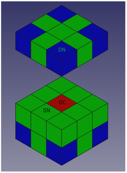
Figure 1. Types of neighboring cells for the calculation of the neighborhood indicator. The types OC, SN, DN are weighted differently in the calculation.

In the first step, we calculate octree codes for every point in D depth and store them in array OCCODE. In the next step, we create an array (OCSPACE, that represents the octree space in D depth and will store the number of points in the octree cubes—the shape of this array is $[2^{D\ast 3},2]$. Next, we run a quicksort on array OCCODE and determine the points for the unique octree code values in the array OCC (the length m of the OCC array is, on average, 0.5 percent of the length of the original point cloud array), and the number of the unique values in the OCCcount array. The structure of the arrays is

$$OOC:[occod{e}_1,occod{e}_2,\dots ];OCCCount:[number Of Point{s}_1,number Of Point{s}_2,\dots ].$$

(2)

Now, we iterate over the OCC array i: = 0 to m (m = length of OCC), fill the corresponding OCSPACE(OCC[i,0]) array item with OCC[i,1] (the number of points), and increase the neighbor (+X axis) OCSPACE[:,1] item with OCC[i,1]/10, and increase the −X axis OCSPACE[:,1] item with OCC[i,1]/10 and perform it in the Y and Z axis. We perform similarly on the twelve edge neighbors (+X, +Y, Z; −X +Y Z; +X −Y Z;…), but we store the result in OCSPACE[:,1]. With these values, we can calculate the SNC (SN count) and the DNC (DN count) values.

With these values, we can calculate the WEIGHT of the given cell. After the loop, we iterate over the original P array. First, we must look for the index of the correspondent octree cell in the OCC array, and examine the WEIGHT and OCCcount values. We drop the point where OCCcount < OC and WEIGHT < NC.

We named the proposed algorithm the Octree Density outlier filter, in brief OCD. The pseudo code of our algorithm can be seen in Algorithm 1, while Figure 2 provides a visual representation of the filtering. After calculating the extent of the point cloud, octree codes are determined for points at specified depths. We used quicksort to order the octree codes, which is followed by calculating the unique values and the number of these values. After creating a full octree space array, we can compute the outlier indicators, by going through all the elements of the points, we increase the indicator values of the octree space corresponding to the point. After that, you just have to switch the matching indicators back to the original points based on the octree code and then discard the non-matching points according to the thresholds.

Algorithm 1: Octree density outlier removal.

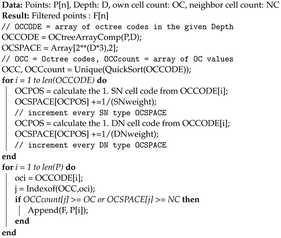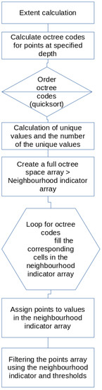
Figure 2. Flowchart of the filtering.

The proposed algorithm needs to apply the quick-sort only once, which can result in saving time. Furthermore, the computation requires only integer arithmetics and does not suffer from the exponential growth of time when the point number increases.

4. Testing Results

We have tested our algorithm on point clouds with different sizes using numbers from different ranges (see Table 4). The first three sample scans were received from Geodezia Ltd. and represent buildings. Mobile scan was created with a Leica Pegasus, while the two industrial point clouds were acquired with a Leica ScanStation P20. The last point cloud about a temple was downloaded from the E57 sample library (http://libe57.org/data.html (accessed on 1 July 2023)). The point cloud of an industrial area is about 39 times larger than the smallest one used for testing. The numerical values are described with digits ranging between five and eight.

Table 4. Sample scans used for testing.

Scan Name	Number of Points	Digit Counts
Industrial area	330,973,927	5
Mobile scan	79,338,713	8
Industrial hall	28,279,109	5
Temple	8,484,455	6

4.1. Testing the Proposed Algorithm on Different-Sized Point Clouds

Each of the following figures (Figure 3, Figure 4, Figure 5 and Figure 6) consists of two images: the left-hand one shows the original point clouds, while the right-hand one is the point cloud after running OCD (the clouds are colored with a height ramp). Figures prove that our algorithm could cope with removing outliers caused by vegetation, measured points with a low incidence angle, points resulting from device positioning error. The most spectacular difference can be observed on the mobile scan (Figure 4); this point cloud has a typical scanner positioning error that results in semicircular outlier points. All of these points were removed by our algorithm successfully.

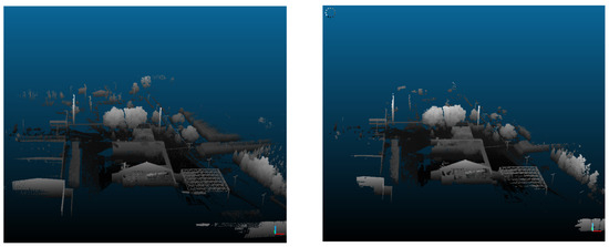
Figure 3. Industrial area (original and filtered). The distant, low point density spots have disappeared.

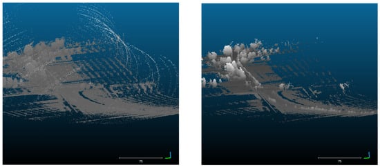
Figure 4. Mobile scan (original and filtered). Circular measurement errors from mobile measurement removed by the filter.

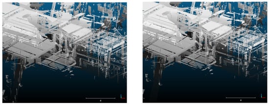
Figure 5. Industrial hall (original and filtered). The distant, low point density spots have disappeared.

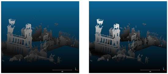
Figure 6. Temple (original and filtered). Distant noise points disappeared, extent reduced.

The next step in evaluating our algorithm is to compare its time complexity to some of the tools in open source packages. To accomplish this, the following frequently used algorithms were selected: PCL SOR, PDAL, Open3D SOR, and Scikit-LOF.

We compared the running times without the time needed for file input/output. The test was executed on a desktop computer AMD R2700X CPU with 32 GB RAM. Only one core was used to run the algorithms except for the Open3D SOR algorithm, where we also tested using three cores. Nevertheless, we have to remark that OCD was written in Python (applying NumPy library), while the others are compiled C/C++ codes. As Table 5 demonstrates, only OCD could complete the outlier detection faster than one hour each cloud. Waiting for the output of an algorithm longer than one hour is meaningless, which is why we aborted these tests; they are designated by an asterisk in the table. Considering the running times, OCD performed well. The current OCD is written in Python, so it could be even faster if it were rewritten and compiled in C, which is one of our future goals. Another development possibility is to make an adaptive parameter setting for more comfortable usage.

Table 5. Running times in sec (*: Running time > 1 h, **: Stopped with memory error).

Sample	PCL (1 Core)	PDAL (1 Core)	Open3D (8 Core)	Open3D (1 Core)	Scikit-LOF (1 Core)	OCD (1 Core)
Industrial area (330 M)	*	*	*	*	**	65
Mobile scan (79 M)	268	*	150	977	**	44
Industrial hall (28 M)	84	*	*	*	218	4
Temple (8 M)	27	207	5	31	51	14

4.2. Testing the Proposed Algorithm on Noisy Point Clouds

Since our algorithm seemed promising according to the test results, we made another comparison with ROL to explore how many points will be removed as an outlier if the point cloud is noisy. Therefore, we randomly added different amounts of noise to three point clouds and then applied our proposed algorithm with different parameterizations (see Table 6). Table 7 lists the parameters used for testing the efficiency in the case of noisy point clouds of different sizes. Although the proposed algorithm is designed to remove outliers, it could remove a remarkable amount of noise and result in a similar number of kept points to the ROL filter.

Table 6. Performance on noisy point clouds.

Original Point Number	Number of Added Noisy Point	Total Point Number to Be Tested	Kept Point Number of OCD (1)	Kept Point Number of OCD (2)	Kept Point Number of ROL
3,000,047	60,000	3,060,047	3,010,962	3,010,755	3,003,464
1,372,245	30,000	1,402,245	1,373,411	1,373,113	1,369,036
155,201	3000	158,201	151,207	151,064	151,175

Table 7. Parameter settings of the algorithms.

Original Point Number	OCD (1)	OCD (2)	ROL
3,000,047	cubesize: 14.28 OC: 8 NC: 12	cubesize: 12.70 OC: 8 NC: 13	Radius: 39.69 EPS: 20
1,372,245	cubesize: 0.03 OC: 8 NC: 12	cubesize: 0.0276 OC: 8 NC: 13	Radius: 0.085 EPS: 20
155,201	cubesize: 0.018 OC: 8 NC: 12	cubesize: 0.016 OC: 8 NC: 13	Radius: 0.05 EPS: 20

4.3. Sensitivity Test with Generated Outliers

In our last sensitivity test, we added 1000 random points to the Stanford Bunny point cloud and tested the results of two different parameterizations (see Table 8). The test shows that the FPR indicator of the algorithm can detect real points incorrectly, so this feature should be improved in further development. For real TLS point clouds, this error is not so significant, so it does not hinder the use.

Table 8. Parameter settings for the sensitivity test.

Test	OCD Depht = 9, OC = 2, NC = 0	OCD Depht = 7, OC = 13, NC = 368	ROL Eps = 10, Radius = 0.00169
FPR	77.411	3.847	0
FNR	0	0	0.00006
TPR	0.9262	0.9963	1
TNR	1	1	0.993

Using parameters that are too strict (high OC or NC) will produce many false negatives, while more permissive parameterization (low OC or NC) will increase the number of false positives. The octree depth should be kept between 7 and 9. A small depth or a small OC number will leave local outliers. Increasing the octree depth also has an impact on speed; a larger octree depth results in a slightly slower execution.

4.4. Further Development

The algorithm can be run in parallel for computing the main loop or octree codes; the most obvious method is to parallelize based on spatial segmentation. We plan to improve the goodness of filtering by running the algorithm multiple times in succession. This can be done with more permissive parameters, or by slightly shifting (in random or per-axis direction) or increasing the total extent (depending on the octree depth)—the latter being a more secure solution, better approximating the original ROL. These improvements increase the runtime only linearly due to the time complexity of O(n).

5. Discussion

Point clouds created with laser scanners can be huge, making working with them hard and long. Since industry prefers having digital models about real objects, and these objects can be massive, the size of the point clouds tends to be larger and larger. One typical issue when working with these large scans is to remove outliers. Outliers are points that must be excluded from further processing based on their location. The time needed for preprocessing is critical and plays an important in the industry. You can save time by using more resources (more memory, more CPU cores, etc.) and also by applying more efficient algorithms. Our goal was to propose an algorithm to eliminate outliers with a complexity that does not increase exponentially with the increase in the point cloud size.

Our algorithm, called Octree Density outlier filter (OCD), is fast and works well on various-sized point clouds. We could reduce the computational demand by introducing a new method to find outliers while its parameterization and output are similar to the ROL filter. The test results show that the running time is not growing exponentially with the point cloud size, which is a noticeable advantage of the algorithm. We compare the performance of our algorithm with that of other algorithms (see Table 5) and found a very promising quickness. We also have to mention that only our algorithm could complete the computation within one hour in the case of the four tested point clouds. In practice, we have already used OCD on terabytes of data, and its application saved us lots of time. It gives appropriately good filtering like the ROL/SOR filter but runs faster than those. The algorithm is implemented in Python currently, but we would like to implement it in C too, which will result in becoming faster. Applying adaptive parameter settings is also a promising opportunity to make the usage of OCD more comfortable.

6. Conclusions

The algorithm was successfully run on a database containing several terabytes of poor quality point clouds (containing outliers and distant reflections)—even the extents in the original point clouds were unusable due to errors. With this amount of data, the PCL library filter, which had been the only one used so far, took four weeks to run, while the new algorithm ran in a day and a half, after which the extents were completely fine. As Table 5 shows, the proposed algorithm performs well compared to PCL, PDL, Scikit-LOF. Open3D running in eight cores was faster only in the case of 8M points, but we have to note that OCD was run in one core only. The ultimate goal is to produce a Python module available under the LGPL using the algorithm, which others can use to preprocess extremely large point clouds or filter streaming point cloud data.

References

- Vic Barnett, T.L. Outliers in Statistical Data; John Wiley & Sons: Hoboken, NJ, USA, 1977. [Google Scholar]
- Le, M.H.; Cheng, C.H.; Liu, D.G. An Efficient Adaptive Noise Removal Filter on Range Images for LiDAR Point Clouds. Electronics 2023, 12, 2150. [Google Scholar] [CrossRef]
- Wang, W.; You, X.; Chen, L.; Tian, J.; Tang, F.; Zhang, L. A Scalable and Accurate De-Snowing Algorithm for LiDAR Point Clouds in Winter. Remote Sens. 2022, 14, 1468. [Google Scholar] [CrossRef]
- Wu, Y.; Sang, M.; Wang, W. A Novel Ground Filtering Method for Point Clouds in a Forestry Area Based on Local Minimum Value and Machine Learning. Appl. Sci. 2022, 12, 9113. [Google Scholar] [CrossRef]
- Chen, C.; Guo, J.; Wu, H.; Li, Y.; Shi, B. Performance Comparison on Filtering Algorithms for High-Density Airborne LiDAR Point Clouds over Complex LandScapes. Remote Sens. 2021, 13, 2663. [Google Scholar] [CrossRef]
- Han, X.F.; Jin, J.S.; Wang, M.J.; Jiang, W.; Gao, L.; Xiao, L. A review of algorithms for filtering the 3D point cloud. Signal Process. Image Commun. 2017, 57, 103–112. [Google Scholar] [CrossRef]
- Ben-Gal, I. Outlier detection. In Data Mining and Knowledge Discovery Handbook; Maimon, O., Rokach, L., Eds.; Springer: New York, NY, USA, 2005; pp. 131–146. [Google Scholar]
- Hodge, V.J.; Austin, J. A Survey of Outlier Detection Methodologies. Artif. Intell. Rev. 2004, 22, 85–126. [Google Scholar] [CrossRef]
- Cateni, S.; Colla, V.; Vannucci, M. Outlier Detection Methods for Industrial Applications. In Advances in Robotics, Automation and Control; BoD—Books on Demand: Norderstedt, Germany, 2008; pp. 265–282. [Google Scholar]
- Yoon, Y.; Cho, Y.; Park, J.; Lyu, J.; Park, K. Accuracy improvement of Pulsed LiDAR using an Adaptive Radius Outlier Removal Algorithm. In Advances in Nano, Bio, Robotics and Energy (ANBRE19); 2019. Available online: https://pubmed.ncbi.nlm.nih.gov/34263788/ (accessed on 17 September 2023).
- Duan, Y.; Yang, C.; Li, H. Low-complexity adaptive radius outlier removal filter based on PCA for lidar point cloud denoising. Appl. Opt. 2021, 60, E1–E7. [Google Scholar] [CrossRef] [PubMed]
- Cui, H.; Wang, Q.; Dong, D.; Wei, H.; Zhang, Y. Fast outlier removing method for point cloud of microscopic 3D measurement based on social circle. Appl. Opt. 2020, 17, 8138–8151. [Google Scholar] [CrossRef] [PubMed]
- Balta, H.; Velagic, J.; Bosschaerts, W.; Cubber, G.D.; Siciliano, B. Fast Statistical Outlier Removal Based Method Outdoor for Large 3D Point Clouds of Environments Method Outdoor for Large 3D Point Clouds of Environments Outdoor Environments. IFAC-PapersOnLine 2018, 51, 348–353. [Google Scholar] [CrossRef]
- Atanassov, R.; Bose, P.; Couture, M.; Maheshwari, A.; Morin, P.; Paquette, M.; Smid, M.; Wuhrer, S. Algorithms for optimal outlier removal. J. Discret. Algorithms 2009, 7, 239–248. [Google Scholar] [CrossRef]
- Breunig, M.M.; Kriegel, H.P.; Ng, R.T.; Sander, J. LOF: Identifying Density-Based Local Outliers. In Proceedings of the 2000 ACM SIGMOD international conference on Management of data, Dallas, TX, USA, 16–18 May 2000; Volume 29, pp. 93–104. [Google Scholar]
- Lipman, Y.; Cohen-Or, D.; Levin, D.; Tal-Ezer, H. Parameterization-free Projection for Geometry Reconstruction. ACM Trans. Graph. 2007, 26, 22-es. [Google Scholar] [CrossRef]
- Ning, X.; Li, F.; Tian, G.; Wang, Y. An efficient outlier removal method for scattered point cloud data. PLoS ONE 2018, 18, e0201280. [Google Scholar] [CrossRef] [PubMed]
- Narváez, A.L.; Narváez, N.E.L. Point cloud denoising using robust principal component analysis. In Proceedings of the International Conference on Computer Graphics Theory and Applications, Setúbal, Portugal, 25–28 February 2006; pp. 51–58. [Google Scholar]
- Nurunnabi, A.; West, G.; Belton, D. Outlier detection and robust normal-curvature estimation in mobile laser scanning 3D point cloud data. Pattern Recognit. 2015, 48, 1404–1419. [Google Scholar] [CrossRef]
- Han, X.F.; Jiang, W.; Jin, J.S.; Wang, M.J. Guided 3D point cloud filtering. Multimed. Tools Appl. 2018, 77, 17397–17411. [Google Scholar] [CrossRef]
- Zhao, Y.; Nasrullah, Z.; Li, Z. PyOD: A Python Toolbox for Scalable Outlier Detection. J. Mach. Learn. Res. 2019, 20, 1–7. [Google Scholar]
- Goldstein, M.; Dengel, A. Histogram-based Outlier Score (HBOS): A fast Unsupervised Anomaly Detection Algorithm. In Proceedings of the 35th German Conference on Artificial Intelligence, Saarbrücken, Germany, 24–27 September 2012. [Google Scholar]
- Le, M.H.; Cheng, C.H.; Liu, D.G.; Nguyen, T.T. An Adaptive Group of Density Outlier Removal Filter: Snow Particle Removal from LiDAR Data. Electronics 2022, 12, 2993. [Google Scholar] [CrossRef]
- Knox, E.M.; Ng, R.T. Algorithms for Mining Distance-Based Datasets Outliers in Large Datasets. In Proceedings of the International Conference on Very Large Data Bases, New York, NY, USA, 24–27 August 1998; pp. 392–403. [Google Scholar]
Disclaimer/Publisher’s Note: The statements, opinions and data contained in all publications are solely those of the individual author(s) and contributor(s) and not of MDPI and/or the editor(s). MDPI and/or the editor(s) disclaim responsibility for any injury to people or property resulting from any ideas, methods, instructions or products referred to in the content. |
© 2023 by the authors. Licensee MDPI, Basel, Switzerland. This article is an open access article distributed under the terms and conditions of the Creative Commons Attribution (CC BY) license (https://creativecommons.org/licenses/by/4.0/).