Appendix A.1
To calculate deep distance, we need to extract deep features for video frames from pre-trained ImageNet models. To select the best ImageNet model for feature extraction of our cow teat videos, we conducted extensive experiments with 12 frequently used ImageNet models. We use the layer prior to the last fully connected layer to extract deep features. These 12 ImageNet models are AlexNet [
45], VGG16 [
47], VGG19 [
47], GoogLeNet [
48], DenseNet-201 [
49], ResNet-18 [
42], ResNet-50 [
42] , ResNet-101 [
42] , Inception-V3 [
50], Xception [
51], InceptionResNet-V2 [
52], NASNetLarge [
46].
We also utilize t-SNE [
53] to visualize extracted deep features in 2D space as shown in
Figure A1, but it is still difficult to select the best pre-trained ImageNet model. We thus plot the projected loss from a high dimension space to the 2D space of the t-SNE model in
Figure A2. We observe that ResNet-101 has the smallest projection loss among the 12 models, which suggests that ResNet-101 is a suitable ImageNet model for extracting deep features. However, we still do not know whether the performance of ResNet-101 features of our key frame extraction problem is better than other deep features. We thus report the performance of all 12 models in
Table 2. We first calculate these deep distances and use key frame selection
to select the key frame candidates, then the quality check is performed to remove noisy key frames. We can find that the deep ReseNet-101 distance indeed achieves a higher F score than other models.
Figure A1.
T-SNE visualization of extracted features of 12 ImageNet models from GH060066 video. Blue represents video frames, while green dots are the key frame image position.
Figure A1.
T-SNE visualization of extracted features of 12 ImageNet models from GH060066 video. Blue represents video frames, while green dots are the key frame image position.
Figure A2.
T-SNE projection loss of different ImageNet models. Y-axis denotes the projected loss from high dimension space to the 2D space.
Figure A2.
T-SNE projection loss of different ImageNet models. Y-axis denotes the projected loss from high dimension space to the 2D space.
Appendix A.2. Other Baseline Features
Here, we provide the details of extracting features from other baselines. As shown in
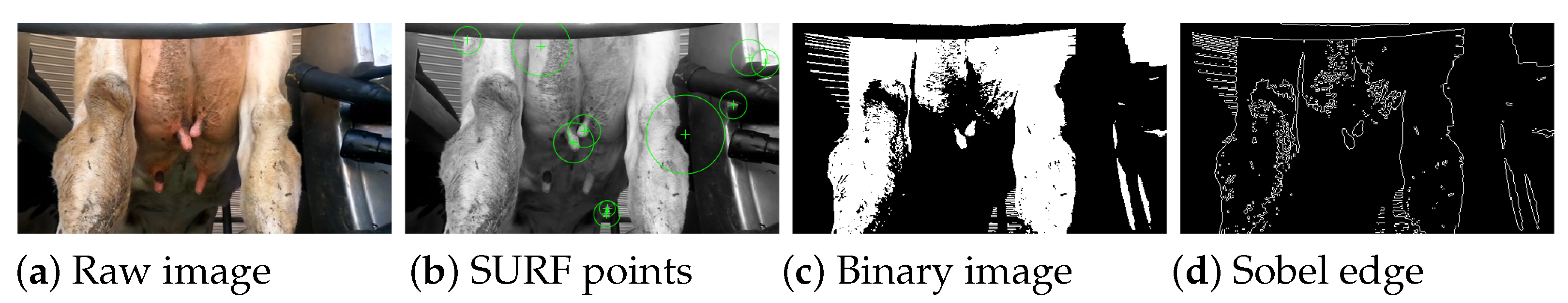
Figure A3, we show SURF detected points, binary image, and edge detection using the Sobel algorithm. In
Figure A3b, we only show 10 of the strongest SURF points, while a total of 500 points are extracted from each video frame and supported key frame images, and there are 64 features for each point. We could extract
SURF features for each image. The SURF distance is defined as follows:
where
refers to the SURF feature extractor and
. In
Figure A3c, we calculate the distance between the binary image of each video frame and support key frame images. The binary distance is defined as follows:
where
B refers to obtaining the binary image. In
Figure A3d, we calculate the distance between edge detection images using the Sobel algorithm of each video frame and support key frame images. The Sobel distance is defined as follows:
where
E refers to obtaining an edge detection image using the Sobel algorithm. After obtaining SURF distance
, binary distance
and Sobel distance
, we use the key frame selection
(the fusion distance
d will be replaced with these three distances, respectively) and perform the quality check process to obtain the final extracted key frames.
Figure A3.
Raw image, SURF 10 strongest points, binary image edge detection with Sobel algorithm image comparison.
Figure A3.
Raw image, SURF 10 strongest points, binary image edge detection with Sobel algorithm image comparison.
We utilize visualize extracted SURF features (
Figure A4) using t-SNE. These frame features (blue dots) are indistinguishable from the non-key frames, as shown in blue in
Figure A1. SURF features also have a higher project loss (1.819) than other ImageNet models. This implies that the performance of SURF features might be lower than different ImageNet models. The average F score of SURF is 32.3 (in
Table 1 of the main paper), which is lower than most ImageNet models.
Figure A4.
T-SNE visualization of extracted SURF features.
Figure A4.
T-SNE visualization of extracted SURF features.
In
Table 1 of the main paper, we also present the result of
, using the SSIM similarity matrix to determine key frames. Specifically, we calculate the SSIM score of the crop teat area of each video frame image and support video key frame image, and then select the highest score to detect the key frames and then perform the quality check process. The SSIM similarity matrix is defined as follows:
where
p represents the teat position area, and
returns the maximum number of each row of the similarity matrix
. Hence,
. We then have a partial new key frame selection function
to determine the key frame candidates as in Algorithm A1. There are two changes, the first is that the input is not the fusion distance
d, but the SSIM similarity matrix
. Secondly, we sort
in a descending order since a more similar teat area is more likely to be a key frame.
Figure A5 shows the process of detecting key frames using new key frame selection function (
) on GH060066 video with similarity matrix
.
| Algorithm A1 Key frame selection mechanism () |
- 1:
Input: SSIM similarity matrix , and redundant frame number - 2:
Output: selected key frame numbers - 3:
= descend-sort() // return the sorted distance and its index - 4:
- 5:
fortodo - 6:
if then - 7:
tem = - 8:
// Assign −1 to () of one key frame - 9:
= tem - 10:
end if - 11:
end for - 12:
- 13:
[] // Remove from the predicted key frames - 14:
return
|
Figure A5.
Key frame extraction with model of GH060066 cow teat video. is similarity matrix. Red dots are the detected key frames, while green dots are the ground truth key frames.
Figure A5.
Key frame extraction with model of GH060066 cow teat video. is similarity matrix. Red dots are the detected key frames, while green dots are the ground truth key frames.
Table A1.
F score (%) and computation time (s) of 12 different ImageNet models (IR: InceptionResNet-V2, NAST: NASNetLarge).
Table A1.
F score (%) and computation time (s) of 12 different ImageNet models (IR: InceptionResNet-V2, NAST: NASNetLarge).
|
Videos | | | | | | |
|---|
| F | Time | F | Time | F | Time | F | Time | F | Time | F | Time |
|---|
| GH060066 | 72.7 | 14.4 | 72.7 | 25.9 | 36.4 | 28.4 | 18.2 | 11.8 | 36.4 | 42.8 | 54.5 | 21.3 |
| GH010063 | 30.8 | 19.0 | 14.3 | 30.5 | 28.6 | 31.0 | 28.6 | 15.7 | 15.4 | 52.4 | 14.3 | 15.6 |
| GH010067 | 22.2 | 18.0 | 60.0 | 27.0 | 20.0 | 27.6 | 66.7 | 14.1 | 22.2 | 46.3 | 60.0 | 14.2 |
| GH020070 | 12.5 | 21.6 | 37.5 | 35.6 | 37.5 | 36.5 | 12.5 | 17.8 | 37.5 | 62.1 | 37.5 | 18.0 |
| GH010069 | 47.1 | 23.9 | 58.8 | 40.4 | 47.1 | 40.7 | 58.8 | 19.9 | 47.1 | 70.6 | 35.3 | 19.8 |
| GH010068 | 52.2 | 32.3 | 27.3 | 56.9 | 43.5 | 61.8 | 43.5 | 28.6 | 52.2 | 101.9 | 43.5 | 25.0 |
| GH010065 | 17.5 | 84.2 | 38.6 | 137.8 | 45.6 | 134.3 | 25.0 | 67.3 | 17.5 | 233.5 | 38.6 | 65.3 |
| GH020071 | 19.2 | 145.3 | 33.3 | 228.1 | 40.5 | 229.4 | 31.0 | 132.3 | 33.3 | 424.3 | 38.4 | 152.3 |
| GH030072 | 25.0 | 181.3 | 8.2 | 228.0 | 32.9 | 242.0 | 22.9 | 142.0 | 25.0 | 428.4 | 35.1 | 157.3 |
| GH040066 | 69.7 | 280.3 | 74.2 | 333.6 | 71.1 | 359.4 | 70.5 | 255.0 | 71.9 | 526.4 | 75.0 | 248.7 |
| GH010071 | 30.9 | 299.4 | 34.7 | 338.3 | 47.4 | 341.9 | 29.2 | 253.2 | 20.6 | 509.7 | 42.4 | 249.2 |
| GH030066 | 43.1 | 282.0 | 33.7 | 322.4 | 39.6 | 343.0 | 33.7 | 242.1 | 26.0 | 505.8 | 51.5 | 249.2 |
| GH010070 | 23.3 | 311.8 | 36.2 | 331.1 | 45.7 | 348.8 | 19.6 | 229.3 | 40.4 | 516.8 | 45.7 | 248.6 |
| GH020072 | 23.1 | 408.7 | 27.2 | 365.4 | 32.4 | 334.9 | 13.6 | 243.3 | 37.3 | 518.6 | 42.3 | 252.1 |
| GH010066 | 36.0 | 327.3 | 41.6 | 325.4 | 45.1 | 338.0 | 33.3 | 247.8 | 31.7 | 495.6 | 45.1 | 252.0 |
| GH020066 | 34.3 | 300.4 | 44.9 | 326.1 | 45.3 | 329.8 | 41.9 | 292.2 | 39.3 | 510.0 | 41.5 | 252.1 |
| GH010072 | 17.1 | 293.5 | 31.8 | 327.3 | 44.9 | 335.6 | 15.1 | 293.2 | 27.2 | 511.3 | 44.9 | 241.7 |
| GH050066 | 47.5 | 277.6 | 54.9 | 330.8 | 54.9 | 347.1 | 21.8 | 264.9 | 25.7 | 511.9 | 47.1 | 250.2 |
| Ave | 34.7 | 184.5 | 40.6 | 211.7 | 42.1 | 217.2 | 32.6 | 153.9 | 33.7 | 337.1 | 44.0 | 151.8 |
| Videos | | | | | | |
| F | Time | F | Time | F | Time | F | Time | F | Time | F | Time |
| GH060066 | 54.5 | 14.3 | 90.9 | 20.8 | 72.7 | 22.5 | 18.2 | 29.5 | 36.4 | 30.9 | 60.0 | 57.7 |
| GH010063 | 14.3 | 18.0 | 28.6 | 20.4 | 14.3 | 28.0 | 14.3 | 37.7 | 0.0 | 36.3 | 42.9 | 94.0 |
| GH010067 | 60.0 | 16.0 | 60.0 | 17.7 | 60.0 | 24.7 | 60.0 | 33.2 | 22.2 | 33.2 | 44.4 | 73.1 |
| GH020070 | 50.0 | 20.9 | 37.5 | 23.0 | 40.0 | 33.2 | 13.3 | 44.4 | 40.0 | 43.9 | 0.0 | 99.9 |
| GH010069 | 47.1 | 22.8 | 58.8 | 26.5 | 12.5 | 39.5 | 35.3 | 50.2 | 37.5 | 49.2 | 0.0 | 122.4 |
| GH010068 | 52.2 | 40.3 | 69.6 | 34.2 | 60.9 | 53.7 | 17.4 | 66.4 | 17.4 | 65.3 | 34.8 | 158.2 |
| GH010065 | 45.6 | 80.9 | 42.1 | 86.7 | 38.6 | 121.2 | 28.1 | 161.0 | 18.2 | 159.5 | 35.1 | 354.4 |
| GH020071 | 32.9 | 140.4 | 43.8 | 188.0 | 28.2 | 218.0 | 28.6 | 250.4 | 14.1 | 268.5 | 33.3 | 554.0 |
| GH030072 | 32.0 | 155.9 | 44.8 | 181.5 | 22.5 | 239.2 | 16.7 | 287.8 | 16.9 | 278.2 | 16.7 | 593.7 |
| GH040066 | 75.0 | 266.7 | 74.2 | 268.7 | 68.9 | 343.4 | 68.2 | 424.3 | 71.9 | 418.9 | 71.9 | 810.6 |
| GH010071 | 50.5 | 269.1 | 53.1 | 272.9 | 35.4 | 369.2 | 16.5 | 440.5 | 20.8 | 402.8 | 30.6 | 807.6 |
| GH030066 | 39.6 | 300.3 | 49.0 | 289.0 | 30.6 | 342.7 | 31.7 | 435.8 | 28.3 | 423.5 | 37.6 | 777.9 |
| GH010070 | 39.6 | 275.0 | 34.3 | 277.9 | 32.4 | 338.3 | 40.0 | 434.7 | 21.2 | 427.0 | 45.7 | 799.3 |
| GH020072 | 45.7 | 287.1 | 46.2 | 281.8 | 15.8 | 326.8 | 31.1 | 420.8 | 14.0 | 425.6 | 29.7 | 818.0 |
| GH010066 | 52.9 | 259.9 | 48.5 | 281.9 | 32.3 | 361.1 | 38.4 | 439.0 | 14.1 | 399.1 | 43.6 | 799.4 |
| GH020066 | 50.5 | 248.3 | 58.5 | 285.2 | 39.6 | 360.4 | 39.3 | 421.7 | 19.4 | 422.8 | 35.5 | 804.0 |
| GH010072 | 44.9 | 272.7 | 37.4 | 286.7 | 36.9 | 344.3 | 21.2 | 423.2 | 29.1 | 448.8 | 36.2 | 780.3 |
| GH050066 | 47.1 | 269.2 | 59.6 | 286.1 | 33.3 | 332.2 | 36.4 | 423.0 | 22.4 | 437.2 | 25.7 | 785.5 |
| Ave | 46.4 | 164.3 | 52.1 | 173.8 | 37.5 | 216.6 | 30.8 | 268.0 | 24.7 | 265.0 | 34.7 | 516.1 |
Appendix A.3. Other Ablation Study
In this section, we show small variants of our UFSKFE model. As shown in
Table A2,
refers to calculating the deep distance using the crop teat area position.
norm means balancing the scale of raw distance and deep distance using L2 norm. In the main paper, we use
and
to balance the scale between them. Here, we instead use the L2 norm, i.e.,
and
. The raw
distance means that we calculate the L2 distance in Equation (
2) of the main paper. It can be denoted as
.
Table A2.
Ablation study of different variants of UFSKFE.
Table A2.
Ablation study of different variants of UFSKFE.
| Video Name | | Feature Norm | Raw Distance |
|---|
| GH060066 | 54.5 | 90.9 | 54.5 |
| GH010063 | 14.3 | 57.1 | 57.1 |
| GH010067 | 60.0 | 44.4 | 44.4 |
| GH020070 | 37.5 | 50.0 | 75.0 |
| GH010069 | 11.8 | 58.8 | 58.8 |
| GH010068 | 26.1 | 69.6 | 69.6 |
| GH010065 | 39.3 | 52.6 | 37.0 |
| GH020071 | 30.6 | 54.1 | 60.3 |
| GH030072 | 19.7 | 46.6 | 36.6 |
| GH040066 | 73.3 | 73.3 | 68.9 |
| GH010071 | 24.5 | 57.7 | 52.1 |
| GH030066 | 38.0 | 49.0 | 56.9 |
| GH010070 | 17.6 | 52.9 | 48.5 |
| GH020072 | 25.0 | 48.5 | 53.8 |
| GH010066 | 21.6 | 62.0 | 56.0 |
| GH020066 | 24.5 | 56.6 | 56.6 |
| GH010072 | 11.5 | 57.9 | 50.9 |
| GH050066 | 35.6 | 64.7 | 57.1 |
| Ave | 31.4 | 58.2 | 55.2 |
From
Table A2, we find that the performance of
(31.4) is much lower than that of
(52.1). The reason is that the small teat area tends to ignore other important background features. The performance of
norm (58.15) is also lower than the simple
norm (63.6 in
Table 2). In addition, the F score of raw
distance (55.2) is slightly lower than the performance of the
distance 55.4 (
Table 2). We can conclude that all proposed strategy in our UFSKFE model is effective in improving the accuracy of key frame extraction in cow teat videos.


