Article

Regression-Based Approach to Test Missing Data Mechanisms

by
Serguei Rouzinov
1,* and
André Berchtold
2
1
Statistique Vaud, 1003 Lausanne, Switzerland
2
Institute of Social Sciences & NCCR LIVES, University of Lausanne, 1015 Lausanne, Switzerland
*
Author to whom correspondence should be addressed.
Submission received: 30 November 2021 / Revised: 16 January 2022 / Accepted: 17 January 2022 / Published: 25 January 2022
(This article belongs to the Section Information Systems and Data Management)

Abstract

:
Missing data occur in almost all surveys; in order to handle them correctly it is essential to know their type. Missing data are generally divided into three types (or generating mechanisms): missing completely at random, missing at random, and missing not at random. The first step to understand the type of missing data generally consists in testing whether the missing data are missing completely at random or not. Several tests have been developed for that purpose, but they have difficulties when dealing with non-continuous variables and data with a low quantity of missing data. Our approach checks whether the missing data are missing completely at random or missing at random using a regression model and a distribution test, and it can be applied to continuous and categorical data. The simulation results show that our regression-based approach tends to be more sensitive to the quantity and the type of missing data than the commonly used methods.

1. Introduction

Data collection is a difficult process for any study and the probability of missing information is huge. It is important that we efficiently deal with missing data (MD) to minimise the bias of estimates and optimise the estimation of the variance of parameters of interest [1]. A variety of methods exist, such as deletion, imputation, or Bayesian methods, but, in general, they are powerful only for certain types of MD [2].
Following the definitions given by Rubin [3], MD are said to be Missing Completely At Random (MCAR) when (1) the probability of the data being missing is unrelated to the variable itself and (2) there is no link between the MD and one or several auxiliary variables, whether collected or not. For instance, a researcher’s typo error when collecting data is considered as MCAR data. When the amount of missing information is limited, data analysts often assume that the data are MCAR, although this type of MD is very rare in reality [2].
MD are said to be Missing At Random (MAR) when the probability of missing (1) is unrelated to the variable itself but (2) can be explained, at least partially, by another variable. For example, workers could be more or less likely to answer questions regarding their income in function of their profession.
MD are said to be Missing Not At Random (MNAR) when they can be explained (at least partially) by the missing values themselves, in addition to other variables. For example, assume that highly paid workers are less likely to report their salary. Even if this situation is intuitively understandable, it is difficult to analyse this type of MD because the information about missingness is both unrelated with the observed data and unobserved, so we cannot determine whether the (unknown) values that are missing are themselves the cause for missingness or not. Moreover, the Rubin’s definition of MNAR includes MAR hypothesis and it is very difficult to distinguish these two mechanisms.
The type of MD is important because it helps to determine which treatment should be applied to MD. Suppose we would like to estimate the IQ score from a specific sample composed of 12 individuals. Table 1 provides complete and incomplete data (four values were deleted for the example). The average of the complete sample is 111.75 and the average of observed values in the incomplete sample is 101.75. In this example, we see that the average of incomplete data is biased, but, of course, in real life we do not have access to the value of MD. This relatively high difference is problematic and it let us suppose that MD are not MCAR. Ignoring them is therefore not the best choice, as the observed values do not form a representative sub-sample of the population. The first step would be to formally test whether these MD are MCAR or MAR. Then, an appropriate treatment of the MD should be applied.
The usefulness of testing MD mechanisms is multiple. First of all, it helps to detect the variables that explain the MD. It is important to identify them to understand the MD mechanism. This helps to choose the best method to handle MD and to extract the maximum amount of information. Moreover, the comprehension of the mechanism generating the MD helps to understand the data and the psychology of respondents. This information can be used in similar studies to decrease the non-response rate. Finally, when the mechanism is known, it is easier to apply a correct method to handle MD.
The usual assumption of MCAR is problematic because in the majority of cases it is false [4], and we can have a relatively large bias if the handling of MD is not appropriate [5]. A common concern with MD is how to determine whether the data are MCAR or MAR. The difference between these two mechanisms was explored in detail by Heitjan and Basu [6]. On one hand, if the data are MCAR, it is possible to use a relatively easy method to analyse the data, such as listwise deletion, if the amount of MD is small [1]. On the other hand, if the data are MAR, they should be treated, for instance, with multiple imputation [3,7], inverse probability weighting [8], or Bayesian methods [9]. Moreover, it is very useful to know which variables explain the presence of MD in order to include them in the final model to answer to the research question. Whether the MAR condition holds is avowedly impossible to test given only observed data [10,11]. In the case of MNAR data, it is impossible to test the mechanism on observed data as well, and thus, it has to be analysed with caution with the use of sensitivity analysis [12].
Several approaches have been developed to test the MD mechanism. Three of them are commonly used currently: the Dixon test [13], the Little test [14] along with its extensions, and the Jamshidian and Jalal test [15,16,17]. These approaches have several advantages and limitations, which are discussed later. Their aim is to test whether the MD are MCAR. It is important to mention that when the method for handling MD is valid for both MCAR and MAR data, then it is also interesting to test the MD mechanisms in order to find additional information, such as the the combination of variables which explain the MD. Thus, a procedure that can extract maximum information from the data is needed, because this is the key to distinguish between MCAR and MAR.
Hereafter, we propose a brief review of the literature on testing MD mechanisms. Then, we develop a complementary approach to test missingness based on regression, which can be applied to both categorical (polytomous) and continuous variables. The aim of our approach is not to test whether MD are ignorable or not, but to correctly differentiate between MCAR and MAR. This is similar to what is performed by existing tests, but one should be aware that the possibility that the MD are actually MNAR is left out. We assume that our data are in a restricted environment so that the amount of information does not tend to infinity. A simulation study demonstrates the behaviour of our approach, the objectives being (1) to compare our approach with the commonly used procedure to test missingness, and (2) to check the robustness of this approach in function of the MD mechanism, the quantity of MD, the sample size, and the data distribution.

2. Existing Approaches for Testing Missing Data Mechanisms

A common concern with MD is how to determine whether the data are MCAR or MAR. Hereafter, we first review the three main tests developed in the literature: the Dixon [13], the Little [14], and Jamshidian and Jalal [15] tests, which aim to test the following hypotheses:
H 0 : M C A R H 1 : M A R

2.1. Dixon Test

One of the easiest tests to determine whether the MD are MCAR is to verify the sample group’s differences [13]. Assume that X 1 and X 2 are two numerical vectors, that a certain percentage of observations in X 1 are missing, and that X 2 is a complete vector. The first step is to divide X 2 into two subsamples, one with individuals where X 1 is observed, and the other with individuals where X 1 is missing:
X 2 = X 2 , m i s   if X 1 is   missing X 2 , o b s   if X 1 is   observed
Next, the means of X 2 , m i s and X 2 , o b s are compared by using a two-sample t-test to check for either significant difference between means (alternative hypothesis) or no difference (null hypothesis). When the null hypothesis is rejected, the conclusion is that the data are not MCAR. This approach can be extended to the more general case with more than two variables. However, even in the case of only two variables, a mean comparison does not allow for a conclusive test, because there could be other differences between the two distributions [5]. Moreover, the mean comparison can be applied only on continuous data. To conclude, this test is inappropriate in the majority of cases and this is why other approaches have been developed.

2.2. Little Test

One of the most used methods to test MD mechanisms was developed by Little [14]. It tests whether the MD in a multivariate Gaussian distributed dataset are MCAR or not. According to this approach, the missingness can be tested by applying a likelihood ratio test asymptotically based on a chi-squared distribution. This test is summarised in the following example. Suppose a dataset D ( n × k ) containing n observations and k variables with a general pattern of MD (each variable can contain a certain amount of MD). Let X i = X i 1 , , X i k be the vector of values for observation i, X o b s , i = X o b s , i 1 , , X o b s , i k the vector of values of observed variables in case i, and r i the indicator for MD for observation i, such that r i = 1 if X i is missing and r i = 0 if X i is observed. This gives the number of distinct MD patterns, J, and the set S j of MD patterns for each j = 1 , , J . Furthermore, μ o b s , j and Σ o b s , j are, respectively, the vector of means and the covariance matrix of observed variables in j. The aim of this approach is to test whether the means of each S j are significantly identical or not. It assumes that the variance is known and uses a likelihood ratio test on the following test hypotheses:
H 0 : ( X o b s , i | r i ) i n d N ( μ o b s , j , Σ o b s , j ) , i S j , 1 j J H 1 : ( X o b s , i | r i ) i n d N ( γ o b s , j , Σ o b s , j ) , i S j , 1 j J
where γ o b s , j is the vector of means of observed variable in j, but, unlike μ o b s , j , is distinct for each pattern j. If the true variance–covariance matrix is unknown, it can be estimated by the maximum likelihood estimator [14].
Although this test is relatively efficient for large samples, it is conservative for small ones. The Little test works well for continuous variables, but categorical data must be recoded into numerical discrete data, a transformation that can rarely be justified theoretically [18]. Two other important problems are that the Little test does not test the dispersion of MD sequence and it is not robust to a deviation from a Gaussian distribution unless the sample size is large enough. The Little test has several extensions, such as a test for repeated categorical or longitudinal data using a stratification procedure [19,20] and a Wald-type test for generalised estimating equations with MD [21].

2.3. Jamshidian and Jalal Test

Another commonly used approach for testing the MCAR hypothesis was developed by Jamshidian and Jalal [15]. The authors aim was to create a test of homoscedasticity, which is a synonym of a test of homogeneity in covariances, that works for data that do not necessarily follow a Gaussian distribution. The first step of this approach is to test the normality and homoscedasticity by using the modified Hawkins [22] test. Jamshidian and Jalal [15] modify it for being able to use it when data are incomplete with the following hypotheses:
H 0 : Normality   and   homogeneity   of   covariances H 1 : Non - normality   or   non - homogeneity   of   covariances
If the null hypothesis is accepted, then the data are considered normal and with a homogeneity of covariances and, without additional information, MD can be considered as MCAR. On the other hand, when the modified Hawkins test is rejected, data can be either: (1) non-normal and with a homogeneity of covariances; (2) normal and with a non-homogeneity of covariances; or (3) non-normal and with a non-homogeneity of covariances. The next step after the rejection of the modified Hawkins test is to decide whether the data are normally distributed or not. On one hand, if the researcher assumes that data follow a normal distribution, then there is no other choice but to reject MCAR hypothesis, because (1) and (3) are excluded. On the other hand, if it is impossible to make such an assumption, then Jamshidian and Jalal [15] developed a non-parametric pairwise variable (NPV) procedure with the following test hypothesis:
H 0 : Homogeneity   of   covariances H 1 : Nonhomogeneity   of   covariances
If the null hypothesis cannot be rejected, then the homogeneity of covariances cannot be rejected as well as the non-normality; consequently, MD are considered to be MCAR. When the test is rejected, then the MCAR hypothesis is rejected as well. However, in this last case no test conclusion can be made about normality. First, each variable is divided in two groups based on the unobserved and observed cases of the variable. The first part consists of observed values and the the second part consists of missing values. Then, the Scholz and Stephens [23] rank-based test or the Anderson and Darling [24] k-sample test is applied to the two parts of the variable to evaluate the equality of distribution between the subsamples. This is performed K ( k 1 ) times, where k is the number of variables and K is the total number of partly observed variables. Thus, the tests are performed simultaneously, which can be complicated when k > 2 [25]. Moreover, because this test has a relatively low power to reject Type I errors [26], Jamshidian and Jalal proposed to use the Benjamini and Hochberg [27] test to fix this issue. More details about the NPV test can be found elsewhere [16].
Finally, the rejection of both the Hawkins and NPV tests gives evidence against the MCAR hypothesis.

2.4. Comparison of the Three Tests

These three approaches for testing MD mechanisms have various limitations. The Dixon test is a very simple and understandable approach, but it is problematic because of (1) the collinearity aspect when there are more than two variables and (2) the non-use of the dispersion within the test. The Little test is the most used approach and it is available in the majority of statistical software. However, it can accept the MCAR hypothesis as soon as there is no difference in means between two subsets, which is not always sufficient because a difference can exist in terms of distribution with no difference in means. Furthermore, it is not robust to a deviation from a Gaussian distribution unless the sample size is large enough. The Jamshidian and Jalal procedure takes into account the dispersion of the data, it does not assume data normality, and no large sample size is required. Nevertheless, its structure is relatively complicated to implement because it uses a combination of two tests and it is non-intuitive for end users. Finally, none of the three tests is really appropriate for categorical data, and they have difficulties dealing with data with a relatively low number of MD. Therefore, the objective of this article is to provide an alternative and complementary approach to these tests by (1) testing the distribution rather than the mean of the variables with MD, and (2) allowing for the approach to be adapted to any type of variables, continuous or categorical.

3. Regression-Based Approach

This section presents our regression-based (RB) approach for testing the following hypotheses:
H 0 : M C A R H 1 : M A R
First, the procedure is described for the continuous case and then the binary and categorical cases are described.

3.1. Principle

Consider a dataset with n observations and k variables. Suppose that only one variable, X 1 , has MD and the other variables are fully observed. Let A be the subset of completely observed data, and let B be composed of observations missing on X 1 but fully observed on X 2 , X 3 , X k (Figure 1). X 1 , o b s A is the observed part of X 1 , and X 1 , m i s B is the missing part of X 1 . The objective is to compare the distribution of X 1 , o b s A and X 1 , m i s B , but since data are unobserved on X 1 , m i s B , a regression model is built to explain X 1 , o b s A from A. Then, this model is used to make predictions X 1 , m i s A ^ and X 1 , o b s B ^ for both X 1 , o b s A and X 1 , m i s B .
In practice, a regression model is defined on the fully observed data (part A of Figure 1):
X 1 , o b s A = g 1 ( X 2 A , X 3 A , , X k A )
where X 2 A , , X k A are the fully observed variables from A and g 1 ( . ) is a link function that depends on the type of X 1 . Interaction terms can also be included in the model.
The next step of the RB procedure is to compare X 1 , o b s A ^ and X 1 , m i s B ^ according to the data type. Regression (1) provides a set of estimated coefficients, β ^ A . β ^ A and A are used to predict X 1 , o b s A , and then β ^ A and B are used to predict X 1 , m i s B , to obtain two sets of predicted values, X 1 , o b s A ^ and X 1 , m i s B ^ . This means that the same set of coefficients is used to predict the observed and missing data.
The difference in distribution between X 1 , o b s A ^ and X 1 , m i s B ^ is the key element of the RB approach to accept or reject the hypothesis that data are MCAR. If the MD are truly MCAR, their presence on the response indicator variable X 1 cannot be explained by other available variables in the dataset. However, if the data on this variable are MAR, some information obtained from the other variables should at least partially be able to explain the presence of MD. Consequently, there should be differences between A and B on variables X 2 , , X k , and these differences should imply a difference between X 1 , o b s A ^ and X 1 , m i s B ^ . When the null hypothesis is accepted, it is assumed that the missing part of data on the dependent variable is MCAR.

3.2. Continuous Case

X 1 , o b s A ^ and X 1 , m i s B ^ are compared in function of the type of X 1 . A linear regression is used to estimate Equation (1) when X 1 is numerical, and the general Kolmogorov and Smirnov (KS) test is applied [28] to compare the estimated values. However, other less usual tests could be used, because the KS test is known to be limited for different reasons, one of them being that it has problems when data are not normally distributed [29]. An interesting alternative could be the Cucconi test [30] because it is generally more powerful than other non-parametric distribution tests and the assumption about the normality of the data is not required. It is available in the R software [31]. Other alternatives, such as the Wilcoxon–Mann–Whitney procedure (a general non-parametric test, [32]) or the Kruskal–Wallis approach (for ordinal data, [33]), could also be used. We advise the use of the Kolmogorov–Smirnov test when data are normally distributed and the Kruskal–Wallis approach when data are ordinal.
Notice that the quality of the regression model used to compute the two sets of predicted subsamples is not essential for the test to perform well. What is essential is, as with the Little, the Dixon, and the Jamashidian and Jalal tests, the inclusion of all explanatory variables relevant to the missingness of data on the response indicator variable of X 1 . When such explanatory variables are not sufficient to explain the variations in the dependent variable, the model fit can be low even if the auxiliary variables are associated with missingness.

3.3. Binary Case

Suppose that the variable with MD, X 1 , is binary with two categories, a and b. In this case, Equation (1) becomes a logistic regression:
π l r = g 2 ( X 2 , o b s A , X 3 , o b s A , , X k , o b s A )
where g 2 ( . ) is the link function and π l r is:
π l r = log p 1 p
with p = P r ( X 1 , o b s = a ) and 1 p = P r ( X 1 , o b s = b ) . Then, the predicted probabilities are computed by using the predicted coefficients β 0 ^ , , β k ^ from model (2):
P r ^ ( X 1 , o b s = a ) = exp ( β 0 ^ + β 1 ^ X 2 A + + β k ^ X k A ) 1 + exp ( β 0 ^ + β 1 ^ X 2 A + + β k ^ X k A )
P r ^ ( X 1 , m i s = a ) = exp ( β 0 ^ + β 1 ^ X 2 B + + β k ^ X k B ) 1 + exp ( β 0 ^ + β 1 ^ X 2 B + + β k ^ X k B )
P r ^ ( X 1 , o b s = b ) = 1 P r ^ ( X 1 , o b s = a )
P r ^ ( X 1 , m i s = b ) = 1 P r ^ ( X 1 , m i s = a )
Then, the differences between (3) and (4) and between (5) and (6) must be tested using the KS test, because the acceptance or rejection of the test for one category does not automatically imply the acceptance or rejection of the test for the other category. This procedure requires two tests (number of categories), and thus the problem of simultaneity of tests should be addressed. A general Bonferroni-type method could be used. However, this procedure is known to have a low power to reject incorrect null hypotheses [26]. To deal with this problem, we propose adjusting the p-values of the KS test by applying the Benjamini and Hochberg (BH) test [27]. If the hypothesis of no significant distribution differences is not rejected for both categories, then the MD are assumed to be MCAR. Otherwise, it is supposed that the MD are not MCAR.

3.4. Categorical Case

Consider the more general case, where the variable with MD, X 1 , is categorical (or polytomous) with z > 2 modalities ( z = 1 , , Z ). A multinomial regression model must then be used. In some cases, an ordinal regression can be considered, but it is often impossible to assume the same gaps between modalities [34], so the multinomial model is generally preferred.
After the prediction process based on the multinomial regression, the difference between predicted probabilities needs to be verified with the KS and BH tests:
P r ^ ( X 1 , o b s = z ) d P r ^ ( X 1 , m i s = z )
The number of comparisons is equal to the number of categories, so that there are J KS and BH tests, because the acceptance or rejection of the first J 1 categories does not automatically imply the acceptance or rejection of the test for the last category. The BH test is always conducted to avoid the problems due to multiple comparisons. If all J KS and BH tests accept the equality of distributions, then we conclude that the MD for the incomplete variable are MCAR. Otherwise, the null hypothesis is rejected.

3.5. Discussion

In contrast to the existing approaches for testing missing data mechanisms which consider the mean [13,14] or the covariance [15], we developed a regression-based approach, which can be applied to either continuous or categorical data. A related, but different, procedure was also proposed in the literature. It consists of dichotomising the variable with MD between observed and non-observed values, and to apply a logistic regression model [35,36]. However, this method has never been applied on a large scale, and it is not proposed in the commonly used statistical software or in textbooks as a standard method.
The RB method assumes that only one variable in the dataset has MD. Obviously, this situation rarely occurs in reality. One possibility is to replace the MD of independent variables in the regression model using imputation [3], but imputing data before testing to determine the type of MD is problematic because wrong imputations can modify the relationship between the cause of the MD and the MD themselves, thus limiting the probability of identifying the real MD type. A possible solution to this issue is an iterative procedure composed of two steps: an initialisation and an iterative phase. We describe this procedure in the case of single imputation, but it can be used with multiple imputation as well. During the initialisation step, the RB approach is first applied to one of the variables with MD using only the variables without MD as predictors. Then, in function of the result of the RB test, the MD are imputed with respect to their mechanism: a random draw from observed data is used to replace MCAR data, and MAR data are imputed using the chained equation principle [37]. An additional complete variable is then available. Next, a second variable with MD is tested for missingness, using the imputed variable and the variables without MD. This procedure is repeated until the data are fully completed. Next, the RB approach is iteratively applied to each variable with MD, using all other variables as predictors in the regression model (including imputed variables). This is essential, because any change between two iterations can have an impact on the prediction of the dependent variable. If the test result for a variable with MD differs from that of the previous iteration, the MD are imputed again. At the end of each iteration, the pattern of MD is computed again. This step is repeated until no differences are found between the MD patterns of two successive iterations. It must be noted that convergence is not certain, so a maximal number of iterations has to be set. This procedure is applied to a real example in Section 5.

4. Simulation Study

We describe hereafter a simulation study demonstrating the behaviour of the RB test.

4.1. General Setting

In this section, we compare the behaviour of the Regression-based approaches with the more standard Little, Dixon, and Jamshidian and Jalal procedures (see Dixon [13], Little [14] and Jamshidian and Jalal [15]). Two sets of experiments, consisting of independent and correlated data, were designed for this comparison:
  • Experiment set 1: independent data:
    • Continuous data with a U ( 0 , 1 ) distribution;
    • Continuous data with a N ( 0 , 1 ) distribution;
    • Binary data with a Bernoulli distribution B ( 1 , 0.4 ) ;
    • Polytomous data with a B ( 1 ; 0.1 , 0.3 , 0.6 ) distribution.
  • Experiment set 2: correlated data:
    • Continuous data with different uniform and normal distributions.
In the case of independent data, a set of 10 variables ( X 1 , , X 10 ) with the given distribution was first randomly generated, X 1 being then modified to include a missing part, and the nine other variables being used as explanatory factors in the regression models. In the case of correlated data, after generating the initial set of 10 variables, four variables were randomly selected between X 2 and X 10 (noted X s e l _ 1 , , X s e l _ 4 ). Then, these four variables were transformed as follows to correlate them with the dependent variable X 1 :
  • X s e l _ 1 = ζ U ( 0 , 3 ) X 1 + ζ U ( 0 , 1 ) ;
  • X s e l _ 2 = ζ U ( 0 , 0.5 ) X 1 2 + ζ U ( 0 , 1 ) ;
  • X s e l _ 3 = X 1 + 1 10 + ζ U ( 0 , 1 ) ;
  • X s e l _ 4 = X 1 3 + ζ N ( 0 , 1 ) ζ U ( 0 , 1 )
where ζ U ( 0 , 1 ) and ζ N ( 0 , 1 ) are two random vectors generated from, respectively, U ( 0 , 1 ) and N ( 0 , 1 ) distributions, and ζ U ( 0 , 3 ) and ζ U ( 0 , 0.5 ) are two random values generated from, respectively, U ( 0 , 3 ) and U ( 0 , 0.5 ) distributions.
The sample size ranged from 100 to 10,000 and the percentage of missingness on X 1 varied between 1% and 50%. MCAR and MAR mechanisms were studied.

4.2. Simulated Missing Data Mechanisms

Different MD mechanisms were simulated by deleting the observations on variable X 1 , following rules defined to mimic MCAR and MAR situations. Let h denote the percentage of MD generated for X 1 . The algorithms used to generate the MD are described below with examples:
  • MCAR: A random vector ν of size n containing uniformly distributed data between 0 and 1 is generated. Then, all data above the ( 100 h ) th percentile in ν are selected and the corresponding observations in X 1 are replaced with MD.
    Example. Let h = 20 . In this case, X 1 is missing when the random vector ν U ( 0 , 1 ) is larger than its 80th percentile.
  • MAR1: In the first MAR mechanism, the MD for X 1 are caused by only one other variable. One of the variables between X 2 and X 10 , say, X , is randomly chosen to become the cause of the MD for X 1 . Then, all data above the ( 100 h ) th percentile in X are selected, and the corresponding observations in X 1 are replaced with MD.
    Example. Let h = 20 . In this case, X 1 is missing when X is larger than its 20th percentile.
  • MAR2: In the second MAR mechanism, the MD for X 1 are caused by two independent variables. Two variables between X 2 and X 10 , say, X and X k , are randomly chosen as the cause of the MD for X 1 . Then, first, select all data above the ( 100 h / 2 ) th percentile in X and replace the corresponding observations in X 1 with MD. Second, do the same with X k . Since some missing data generated from X k could have already been generated from X , continue to generate MD from X k by going under the ( 100 h / 2 ) th percentile until exactly h percent of data are replaced by MD for X 1 .
    Example. Let h = 20 . In this case, X 1 is missing when X and X k are larger than their 90th percentile. Since some MD generated from X k could have already been generated from X , then the largest values from X k are additionally used until exactly 20% of the data for X 1 are missing.
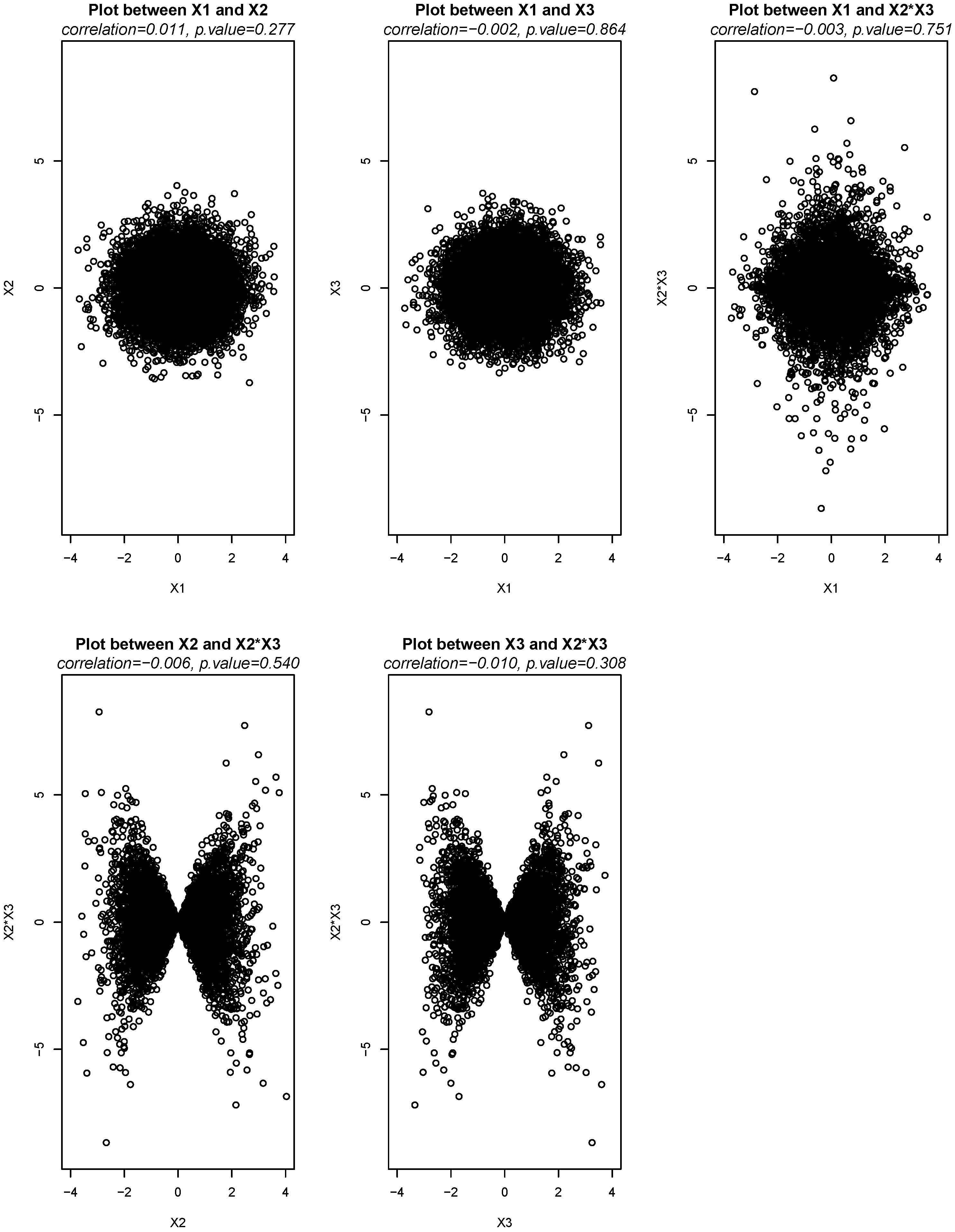
  • MAR3: The third MAR-generating mechanism is quite similar to MAR2, but it uses three different variables to generate MD. The difference with MAR2 is that it uses the second and third variables to build an interaction term (simple multiplication) and generates the second part of the MD from this interaction term rather than from the original variables. The interaction term allows to make the generation of MD more complex and to have an indirect explanation of MD.
    Example. Let h = 20 . In this case, X 1 is missing when X and the interaction between X k and X j (simple multiplication) are larger than their 90th percentile. Since some MD generated from the interaction term could have already been generated from X , then the largest values from X k X j are additionally used until exactly 20% of the data for X 1 is missing.
  • MAR4: The last MAR mechanism is similar to MAR1, except that the MD are caused by an interaction term built from two variables randomly selected from X 2 , , X 10 instead of from only one randomly selected variable.
    Example. Let h = 20 . In this case, X 1 is missing when the interaction between X and X k is larger than its 80th percentile.
Figure 2 and Figure 3 explain the different MD mechanisms on a reduced example with only 4 variables (instead of 10 in the real simulations) and 20 observations. Figure 2 represents a complete dataset composed of four uncorrelated variables, X 1 to X 4 , following a U ( 0 , 1 ) distribution, and of two interaction terms, X 3 X 4 and X 2 X 3 . These interaction terms are a simple multiplication element by element of the generating variables, which is commonly called the Hadamard product [38]. In addition, there is a a random generated vector, ν , that does not belong to the dataset, but that is used to generate MCAR data. The desired quantity of MD is 20% (4 observations). Figure 3 represents the MD mechanisms. For MCAR, the highest four values of the random vector ν are used to assign missing values to X 1 . Then, the original X 2 , , X 4 complete variables are used to define the MD in the different MAR mechanisms. For MAR2 and MAR3, some of the MD can be generated identically from both independent variables. In this case, one or several additional values from the second vector have to be used in order to have exactly 20% of MD for X 1 . That is why three values (instead of two) from the interaction X 3 X 4 are used to generate MAR3 for X 1 . Appendix A presents the R code for (1) the general way to simulate the MCAR and MAR1 to MAR4 mechanisms, and (2) the simulated example from Figure 2 and Figure 3. Notice that the difference between MCAR and MAR mechanisms lies in the fact that the random vector ν , which explains the presence of MCAR data, does not belong to the dataset, so it cannot be used in the regression model of the RB test, while vectors X 1 to X 4 , which explain the presence of MAR data, are in the dataset.

4.3. Simulation Procedure

The main purpose of these simulations is to compare the behaviour of the RB approach with the Dixon, Jamshidian and Jalal, and Little tests. The four approaches were applied to continuous data, and the RB and Little approaches were also applied to categorical data for different MD mechanisms, sample sizes, and percentages of generated MD. For MAR mechanisms, all tests are performed using the nine variables X 2 , , X 10 as explanatory variables in the regression model. Moreover, because the MAR4 mechanism uses only an interaction term, the situation with this interaction variable added to the dataset is also tested (MAR4i). Each situation is replicated 1000 times and the percentage of acceptance of the null hypothesis (MCAR) by each approach is analysed.
Because the data for this simulation study were randomly generated, there is no significant difference between the variables X 2 , , X 10 in part A and in part B of each dataset (see Figure 1). If there was a significant difference between them, the concerned variable would have been a natural candidate for the cause of the MD for X 1 . This trivial case being excluded, the reason for rejecting the null hypothesis of the test can actually be found in the MAR mechanisms described above.
The RBtest [39] package of the open-source statistical software R [40] was used for all computations. The Type I error was set to 5%.

4.4. Experiment Set 1: Independent Data

4.4.1. Uniform Distribution

For continuous dependent variables, two types of dataset were simulated, the only difference being the data distribution:
  • U ( 0 , 1 ) with a sample size of 1000;
  • N ( 0 , 1 ) with a sample size of 1000.
Table 2 summarises the simulation results for MCAR and MAR generating mechanisms when the sample size is 1000 and the data follow a U ( 0 , 1 ) distribution. For this setting, all tests accept the MCAR hypothesis when the MD are really MCAR with a probability close to the degree of confidence of the test (95%). The conclusions diverge between tests for MAR mechanisms. Both the Dixon and Little tests reject MCAR in the majority of cases, while the Jamshidian and Jalal procedure tends to accept MCAR in the presence of a large quantity of MD. In addition, Jamshidian and Jalal accepts MCAR when MAR1, MAR4, and MAR4i are used and for a relatively low quantity of MD as well. This unexpected behaviour is a sign that the Jamshidian and Jalal is not appropriate for all types of MD. There is no definitive explanation for this unexpected behaviour, although the following elements should be considered:
  • The Jamshidian and Jalal procedure uses a combination of two tests: the modified Hawkins test and a non-parametric distribution test. However, there is no adjustment for the total error, which is problematic for simultaneous tests [27];
  • Its procedure is such that when data follow a multivariate normal distribution, the test rejects the null hypothesis more often. Thus, it is impossible to compare the application of the test on different types of data;
  • The construction of the Hawkins test is such that whatever the distribution, when the sample size is relatively small the test fails to reject the null hypothesis (lack of statistical power). This means that when there is a relatively small quantity of MD, it is too easy for the modified Hawkins test to accept the null hypothesis;
  • It is known that non-parametric tests are generally less powerful than parametric ones [41], and the Jamshidian and Jalal procedure uses a non-parametric test to check for missingness.
The same behaviour was also observed for other sets of simulated data. All these considerations lead us to consider that the Jamshidian and Jalal test sometimes has a poor reliability.
Finally, in presence of MAR data the probability of the RB approach to correctly identify this MD mechanism is positively correlated with the percentage of MD. The higher the percentage of MD, the higher the probability of rejecting the MCAR case. This behaviour is not surprising, since the more information (here: missing data), the easier it should be to identify the correct type of MD.

4.4.2. Normal Distribution

Table 3 summarises the simulation results for MCAR and MAR generating mechanisms when the sample size is 1000 and the data follow a N ( 0 , 1 ) distribution. In this setting, all approaches accept MCAR when the MD are truly MCAR. In the case of MAR mechanisms, both the Dixon and Little tests reject MCAR when MD are MAR1, MAR2, MAR3, and MAR4i. On the other hand, the MAR4 has a specific behaviour. This special behaviour is due to the absence of the interaction variable when computing these tests (note that when the interaction is added (MAR4i.) this problem disappears). This difference for the MAR4 case is specific to N ( 0 , 1 ) data as compared to U ( 0 , 1 ) data. To understand this difference between distributions, scatter plots, and Pearson correlation tests were performed between X 1 , the complete variables that form the interaction and the interaction itself. For normal data, Figure 4 shows that there are no significant correlations between the variables that form the interaction ( X 2 and X 3 ) and the interaction ( X 2 X 3 ). This means that when the interaction is not added to the model (MAR4 case), the presence of X 2 and X 3 in the model may not impact on the presence of MD for X 1 (even if they are explained by the interaction). Consequently, there is no other choice but to accept the MCAR hypothesis. The RB approach rejects the MCAR hypothesis less often when the number of MD is relatively low, except for MAR4. The results of the Jamshidian and Jalal procedure show, once again, unexpected behaviour, as explained in the previous section.

4.4.3. Comparison of the Continuous Results

In this subsection, we summarise and graphically compare the simulation results on all continuous data (Figure 5). The left side of the figure represents the results for data following a U ( 0 , 1 ) distribution, while the right side represents data following a N ( 0 , 1 ) distribution. Only the MCAR and MAR1 generated MD mechanisms are presented here.
The MCAR hypothesis is widely accepted by all approaches when data are truly MCAR. For the MAR1 case, the main comparison results are that (1) the Little and Dixon tests always reject the MCAR hypothesis and (2) the Jamshidian and Jalal and RB procedures accept the MCAR hypothesis more often when data follow the N ( 0 , 1 ) distribution.
When there is a small number of MD, it should be more difficult to find a powerful argument to reject the null hypothesis. Thus, the results are not expected to be correct in 100% of cases. Figure 5 shows that the decrease in the percentage of MD has no impact on both Little and Dixon tests. This result is also explained by the strong MAR1 assumption, where MD are completely explained by one variable. The RB approach gives more weight to MCAR data and balances the results in function of the percentage of MD.

4.4.4. Binary Distribution

For data with a dependant binary variable, X 1 has two modalities, [ a ] with probability p = 0.3 and [ b ] with probability 1 p = 0.7. The sample size takes different values in the following set: n = [ 100 ; 250 ; 500 ; 1000 ; 2000 ; 10,000 ] . From 1% to 50% of MD are generated for the dependant incomplete variable X 1 either purely by random (MCAR case) or by using the MAR1 mechanism.
Notice that even if it is used for comparison purpose, the Little test is not really able to test missingness when data are categorical; therefore, categorical data are first transformed into numerical values. The transformed data could be tested by the Jamshidian and Jalal and the Dixon tests as well, but since these approaches were not developed for categorical data, there is no sense in applying them to the categorical case. This argument is also valid for the Little test but, because it is nevertheless commonly used for categorical data in the literature, it was important to compare it with the RB approach.
The results are summarised as percentage of cases in which the null hypothesis, that is the MCAR hypothesis, is accepted. Results are given in Table A1 and Figure 6 (Appendix B). The figure contains five graphics:
  • (a) Represents the results of the RB approach for MAR1 data. It shows how this approach behaves as a function of the quantity of MD and the sample size;
  • (b) Represents the difference between the RB approach and the Little test when the sample size is equal to 100;
  • (c)–(e) are the same as (b), except that the sample size increases respectively to 250, 500, and 1000.
Figure 6a shows that whatever the sample size, the RB approach rejects the MCAR hypothesis more often when the quantity of MD increases. Moreover, the results of the RB approach evolve with the sample size. Moreover, the larger the sample size, the easier it is to reject the MCAR hypothesis. Figure 6b–e show that the Little test and the RB approach tend to be closer in terms of rejection of the MCAR hypothesis (while the data are truly MAR) with an increase in the sample size. Furthermore, the Little test always rejects the MCAR mechanism when the sample size is at least 1000, even when the sample includes a very small percentage of MAR data. However, it may not always be correct to reject MCAR when the percentage of MD is very small, because the information set on which to base the decision is then very small. The relatively strong MAR1 assumption, where MD are completely explained by one variable, could partially explain this result of the Little test.

4.4.5. Multinomial Distribution

For the multinomial case, we consider three modalities { a ; b ; c } for variable X 1 with the following probability of occurrence:
X 1 = a   with   p = 0.1 b   with   p = 0.3 c   with   p = 0.6
For this set of simulations, the sample size is constant and equal to 10,000. Five MD mechanisms are used: MCAR, MAR1, MAR2, MAR3, MAR4, and MAR4i (same algorithms as before).
Table A2 (Appendix B) summarises the results for the Little and RB tests by giving the percentage of acceptance of the MCAR hypothesis. Both tests lead to similar conclusions. They accept the MCAR hypothesis when the data are MCAR in 95% of cases on average and when the MD are MAR, they reject MCAR in the large majority of cases. However, when the total amount of MD is less than 3%, the probability of acceptance of the MCAR hypothesis in the RB approach is larger than 5% when the MD are MAR.

4.5. Experiment Set 2: Correlated Data

Real data are often correlated. It is then important to verify how the tests of MD mechanisms are influenced by the level of inter-variable correlation. Therefore, we simulated one set of correlated continuous data, as explained in Section 4.1.
We applied the RB, Little, and Dixon approaches to verify the impact of the quality of the linear regression models on the results. The regression models for the dependent variable X 1 used the nine other variables as explanatory variables, including variables X s e l _ 1 , , X s e l _ 4 . Table A3, Table A4 and Table A5 present the results for, respectively, the Dixon, Little, and RB approaches with different ranges of R 2 (Appendix C). The R square measure is very helpful to evaluate the quality of a regression model. We used it because we wanted to explore the relationship between the quality of the regression model and the accuracy of the RB test. Table A6 (Appendix C) shows the sample size for each range of the R 2 , given that there are 1000 replications for each percentage of MD and, thus, there are 14,000 datasets. The results show that whatever the level of the R 2 , the three approaches work well for MCAR data because they accept the MCAR hypothesis in 95% of the cases in average. However, for MAR data, the RB approach tends to accept the MCAR hypothesis much more often than when data are independent (whatever the R 2 ), while the Dixon and Little tests always accept the MAR hypothesis. As already noted in the case of independent data, the behaviour of these latter two tests is somewhat strange, since it implies a near-infinite power of the tests, even in presence of a very low amount of information. In contrast, even if the RB test proves sometimes wrong in detecting correctly MAR data, at least its behaviour is related to the R 2 of the model, the probability of obtaining the true result being inversely related to the degree of dependence between data.

4.6. Discussion

For continuous data the results are relatively similar whether the data follow a N ( 0 , 1 ) or a U ( 0 , 1 ) distribution, except for one of the MAR mechanisms (MAR4, N ( 0 , 1 ) ). The percentage of non-observed data is an important factor: the RB and Jamshidian and Jalal approaches tend to accept the MCAR hypothesis more often as compared to the Little and Dixon procedures when there is a relatively large quantity of MAR data.
The RB approach is less conservative than the Little and Dixon tests, while the Jamshidian and Jalal approach seems to be more similar to the RB procedure. However, as explained in Section 4.4.1, the Jamshidian and Jalal approach has an unexpected behaviour, mainly due to its principle based on a combination of two tests. For very small percentages of MD, the MCAR hypothesis is more often accepted by the RB approach.
For the categorical and independent data experiment, only the RB and Little approaches were used, because the other methods are not appropriate for this data type. As shown by the simulations, the Little and RB approaches tend to behave similarly, except that the Little test is less sensible to a variation in the percentage of MD than the RB approach. In the case of a binary incomplete variable and MAR data, neither approach is recommended when n = 100 ; in a conservative approach, a minimum sample size of n = 1000 seems necessary. In the case of a multinomial incomplete variable with three categories and MAR data, there are no important differences between the Little and RB approaches, whatever the MAR mechanism. The RB approach works well even if the number of modalities increases, however the size of each subsample of a category should be at least 100 to achieve plausible results.
When data are correlated, the results for MCAR data are generally very similar to the ones obtained on the independent data: the MCAR hypothesis is accepted in 95% of the situations on average. In the case of U ( 0 , 1 ) data and MAR mechanisms, the different ranges of the R 2 show that the RB approach tends to give too much importance to MCAR data when data are truly MAR (as compared to the Dixon and Little tests). Meanwhile, the Little test always rejects correctly the MCAR hypothesis for both independent and correlated data.

5. Application on Real Data

We apply the four approaches—RB (use of the two step procedure explained in Section 3.5), Dixon, Little, and Jamshidian–Jalal—to test MD mechanisms on a set of variables (completely and partially observed) of the first wave of the Professional Path Survey [42]. The main purpose of this survey was to understand the professional transitions, career pathways, personal experiences, and well-being of employed and unemployed middle-aged adults (25–55 years) living in the French and German speaking regions of Switzerland. The sample size is 1902 (excluding the unit non-responses). The selected variables are listed in Table 4.
For the RB approach, the maximum number of iterations is set to 50. Moreover, given that there is a certain amount of uncertainty in the iterative step of the RB approach (mainly due to the high amount of variables and the multiple imputation by the chained equation method), we replicate the RB procedure 100 times (number of simulations). This gives more credibility to the RB approach when compared to the other tests.
The Dixon test is applied ( K 1 ) K times, K being the number of variables with at least one missing value. Thus, only variables with at least one missing value are tested by the Dixon approach. Two special cases require discussion. First, the test cannot be computed when all MD on one variable are also missing on the second variable. In such a case, we suppose that MD are MAR for not taking the risk of a bad replacement. Second, when both variables have a certain amount of MD in common, in addition to MD that are differently distributed over the two variables, the t-test is applied. This is problematic when the remaining quantity of observed data is relatively low, because it is known that the power of the t-test decreases with the sample size [43].
Table 4 summarizes the results. The variables are listed in the first column. The second column gives the absolute frequency of MD per variable. The third column represents the number of times the MCAR hypothesis is accepted by the RB approach over the 100 simulations. The results of the Dixon procedure are in the fourth column, where the first value is the number of testing variables leading to the acceptance of the MCAR hypothesis and the second value is the number of testing variables leading to the rejection of the MCAR hypothesis. The fifth and sixth columns provide the p-values of the Jamshidian and Jalal and Little procedures, which test missingness using the overall information, and, thus, only one number per test is provided. Note that for the Jamshidian and Jalal procedure, the p-value shown in Table 4 corresponds to the last step of the procedure where the homogeneity of covariances is tested. Of course, in this case, the null hypothesis in the first step of the procedure was rejected.
When the RB approach is applied, there is no ambiguity for self-rated health, number of jobs, income, neuroticism, extraversion, openness, agreeableness, conscientiousness, and education; the MCAR hypothesis is accepted in at least 95% of cases. The conclusion is the opposite for Children, because the MCAR hypothesis is always rejected, and, thus, the MD are supposed to be MAR. Marital status is supposed to be MCAR, because the MCAR hypothesis is accepted in 90% of cases. Results are more contrasted for the two remaining variables; the MCAR hypothesis is rejected in 42% of cases for Household and in 18% of cases for General health. A first naive explanation could be that only the number of MD affects the result, that is there is a higher probability of accepting the MCAR hypothesis when this number is relatively low. For instance, Education has a relatively low number of MD (13) and the RB approach accepts the MCAR hypothesis in 98% of cases. However, this hypothesis does not hold for Household, which contains only 9 missing values and for which the RB approach approximately equally accepts and rejects the MCAR hypothesis over the 100 simulations. Both variables (Household and Education) have a similar and relatively low quantity of MD; however, the difference in the distributions between the acceptance and rejection of the MCAR hypothesis is important.
For the Dixon approach, the results are more contrasted with respect to the RB procedure. For instance the Dixon test always rejects the MCAR hypothesis for the four variables related to personality, while the RB approach accepts MCAR in the large majority of cases. The Little test suggests that these MD are globally not MCAR, but without doing any distinction between variables, while the Jamshidian and Jalal globally accepts the MCAR hypothesis. Such results provide a contrasting conclusion about the type of MD.

6. Conclusions

There are few methods in the literature to test missingness. The most commonly used ones, the Dixon [13], Little [14] and Jamshidian and Jalal [15] methods, are all limited in different ways. This article has described an innovative approach to test MCAR versus MAR data. This method is adapted both to continuous and categorical data. Demonstrating that MD are not MCAR is important because in that case it is generally recommended to use multiple imputation to handle MD, while it is very common in practice to simply delete non-observed data. Moreover, knowing the MD mechanism can help to detect some response patterns and to better understand the data, as well as the psychology of respondents.
Our results show that no test can be universally applied to correctly detect the correct MD mechanism. All tests have difficulties when data are correlated. A limitation of the our approach, but similar to other tests, is that it is not designed to test the MNAR hypothesis. However, in the longitudinal context, the RB approach could be extended to detect non-ignorable MD by combining it with the drawn indicator family of methods [44]. Furthermore, simulations of MAR mechanisms with a weaker link between MD and there explanation would be necessary.
The method developed in this article is not meant to replace existing testing procedures, but to offer an additional tool for scientists and data analysts to check whether their MD are completely randomly distributed over their dataset or not, and to offer them an additional point of view on missingness.

Author Contributions

Conceptualisation, S.R. and A.B.; software development, S.R.; formal analysis, S.R.; interpretation of results, S.R. and A.B.; writing—original draft preparation, S.R.; writing—review and editing, S.R. and A.B.; supervision, A.B. All authors have read and agreed to the published version of the manuscript.

Funding

This publication benefited from the support of the Swiss National Centre of Competence in Research LIVES—Overcoming vulnerability: Life course perspectives, which is financed by the Swiss National Science Foundation(grant number: 51NF40-160590). The authors are grateful to the Swiss National Science Foundation for its financial assistance.

Institutional Review Board Statement

Not applicable.

Informed Consent Statement

Not applicable.

Data Availability Statement

Data from the simulation study can be generated using the R code provided in the appendix. Data from the Professional Path Survey can be downloaded from here: https://www.swissubase.ch/fr/catalogue/studies/12734/17161/overview, accessed on 30 November 2021.

Acknowledgments

Most of this work was completed while Serguei Rouzinov was Ph.D. student within the NCCR LIVES.

Conflicts of Interest

The authors declare no conflict of interest.

Appendix A. R Code for Generated Missing Data Mechanisms

m<-10  # number of variables.
n<-10000   # sample size.
mis<-20  # percentage of missing data on the dependent variable
set.seed(40)
############# MCAR and MAR mechanisms #############
#----------------#
#----- MCAR -----#
#----------------#
X<-matrix(NA,ncol=m,nrow=n)
for (i in 1:m){
X[,i]<-runif(n,0,1)
}
X<-data.frame(X)
X_MCAR<-X
aa<-runif(n,0,1)
X_MCAR[which(aa<=sort(aa)[mis*(n/100)]),1]=NA
#----------------#
#----- MAR1 -----#
#----------------#
X<-matrix(NA,ncol=m,nrow=n)
for (i in 1:m){
X[,i]<-runif(n,0,1)
}
X<-data.frame(X)
X_MAR1<-X
selection<-sample(c(2:ncol(X_MAR1)),1)
x_s<-X_MAR1[,selection] # one sampled independent variable.
q_MAR_1<-quantile(x_s,seq(0,1,0.01))[100-mis+1]
X_MAR1[which(x_s>q_MAR_1),1]<-NA
#----------------#
#----- MAR2 -----#
#----------------#
X<-matrix(NA,ncol=m,nrow=n)
for (i in 1:m){
X[,i]<-runif(n,0,1)
}
X<-data.frame(X)
X_MAR2<-X
selection<-sample(c(2:ncol(X_MAR2)),2)
x_s<-X_MAR2[,selection] # two sampled independent variables.
q_MAR_1<-quantile(x_s[,1],seq(0,1,0.005))[mis+1]
X_MAR2[which(x_s[,1]<q_MAR_1),1]=NA
X_MAR2[which(is.na(X_MAR2[,1])==F)
[which(x_s[which(is.na(X_MAR2[,1])==F),2]<
quantile(x_s[which(is.na(X_MAR2[,1])==F),2],
(mis/2)/(100-(mis/2))))],1]=NA
#----------------#
#----- MAR3 -----#
#----------------#
X<-matrix(NA,ncol=m,nrow=n)
for (i in 1:m){
X[,i]<-runif(n,0,1)
}
X<-data.frame(X)
X_MAR3<-X
selection<-sample(c(2:ncol(X_MAR3)),3)
x_s<-x_s_1<-X_MAR3[,selection] # three sampled independent variables.
x_s<-cbind.data.frame(x_s[,1],x_s[,2]*x_s[,3])
q_MAR_1<-quantile(x_s[,1],seq(0,1,0.005))[mis+1]
X_MAR3[which(x_s[,1]<q_MAR_1),1]=NA
X_MAR3[which(is.na(X_MAR3[,1])==F)
[which(x_s[which(is.na(X_MAR3[,1])==F),2]<
quantile(x_s[which(is.na(X_MAR3[,1])==F),2],
(mis/2)/(100-(mis/2))))],1]=NA
#----------------#
#----- MAR4 -----#
#----------------#
X<-matrix(NA,ncol=m,nrow=n)
for (i in 1:m){
X[,i]<-runif(n,0,1)
}
X<-data.frame(X)
X_MAR4<-X
x_s<-X_MAR4[,sample(c(2:ncol(X_MAR4)),2)] # two sampled independent variables.
x_s<-x_s[,1]*x_s[,2]
q_MAR_1<-quantile(x_s,seq(0,1,0.01))[100-mis+1]
X_MAR4[which(x_s>q_MAR_1),1]=NA
##########################################################
#--------------------------------------------------------#
#----- Simulated example of missing data mechanisms -----#
#--------------------------------------------------------#
##########################################################
set.seed(40)
# 5 variables with a uniform distribution and a sample size of 20
D<-matrix(NA,ncol=5,nrow=20)
for (i in 1:5){
D[,i]<-runif(20,0,1)
}
colnames(D)=c("v","X1","X2","X3","X4") # names of columns
D<-data.frame(D)
D$X3X4<-D$X3*D$X4 #interaction term between X3 and X4
D$X2X3<-D$X2*D$X3 #interaction term between X2 and X3
D<-round(D,digit=3) # 3 digits
# Check for the highest 20% of values for each variable
D_s<-D # sorted data.frame
for (i in 1:ncol(D)){
D_s[,i]<-sort(D[,i])
}
D_s[17:20,c(1,3:7)] # the 4 highest values of each
# variable and interactions,
# except X1

Appendix B. Simulation Results of Experiment Set 1

Table A1. MAR1 and MCAR mechanisms, binary data with p = 0.3 . The percentage of acceptance of the MCAR hypothesis is provided for the Little (L) and regression-based (RB) approaches.
% of MDn = 100n = 250n = 500n = 1000n = 2000n = 10,000
MCARMAR1MCARMAR1MCARMAR1MCARMAR1MCARMAR1MCARMAR1
LRBLRBLRBLRBLRBLRBLRBLRBLRBLRBLRBLRB
50%96.293.9029.894.794.5020.093.995.3011.995.695.909.195.694.706.595.295.703.7
45%96.393.4032.795.494.4021.394.094.6014.296.096.309.895.495.208.396.194.202.5
40%95.994.6035.293.893.7023.994.695.3018.596.195.2012.695.694.809.395.895.403.6
35%96.093.5037.695.195.4024.793.795.8021.495.695.4013.595.594.5010.396.194.804.0
30%96.395.8044.595.096.4027.494.696.6020.696.195.6014.494.594.6011.695.395.103.5
25%95.596.4048.295.696.1032.394.595.3023.096.996.5016.694.494.3011.696.594.704.2
20%95.095.7051.195.495.4035.793.494.8025.295.294.8019.694.195.6012.695.494.705.3
15%95.195.3057.495.294.6043.494.896.1032.795.996.3020.595.694.1016.095.695.107.2
10%96.294.6065.895.795.4052.894.995.6040.396.295.8028.896.395.3022.195.495.307.3
5%96.594.59.679.595.595.0065.894.495.5053.496.296.3039.095.595.6029.695.195.6012.5
4%96.594.732.981.895.595.4070.295.394.4055.195.397.1045.095.495.1034.895.695.2014.4
3%97.394.261.385.095.695.3072.795.295.6063.796.196.3049.195.094.7038.696.393.4017.4
2%97.493.385.387.695.495.05.179.796.194.6070.296.396.0059.295.394.5045.895.795.6020.6
1%99.293.998.593.497.795.057.887.096.695.33.280.597.295.6070.794.096.8058.995.195.8026.6
Table A2. MCAR and MAR mechanisms, B ( 1 , 0.1 , 0.3 , 0.6 ) , n = 10,000 . The percentage of acceptance of the MCAR hypothesis is provided for the Little (L) and regression-based (RB) approaches.
n = 10,000
% of MDMCARMAR1MAR2MAR3MAR4MAR4i
LRBLRBLRBLRBLRBLRB
50%95.294.500000000.100
45%96.195.0000000.100.200
40%95.894.100.300.10000.200.1
35%96.195.700.50000.300.200
30%95.396.200.300.400.100.100
25%96.595.300.200.200.100.300
20%95.496.100.400.400.300.100
15%95.695.300.200.500.600.500
10%95.495.900.801.301.000.300
5%95.196.102.302.803.000.500.2
4%95.696.201.803.405.000.900.6
3%96.396.002.804.304.702.000.2
2%95.796.504.607.008.802.500.9
1%95.195.809.2015.1017.503.902.1

Appendix C. Simulation Results of Experiment Set 2

Table A3. Dixon test, MCAR and MAR mechanisms, U(0, 1), n = 10,000, R 2 [0,1[.
% of MD R 2 [ 0 , 0.05 [ R 2 [ 0 , 0.1 [
MCARMAR1MAR2MAR3MAR4MAR4iMCARMAR1MAR2MAR3MAR4MAR4i
50%94.10000097.400000
45%100.000000100.000000
40%92.90000097.100000
35%76.90000087.900000
30%86.40000087.200000
25%85.70000091.200000
20%96.20000096.400000
15%94.40000094.900000
10%87.50000092.100000
5%100.000000100.000000
4%100.00000097.300000
3%100.000000100.000000
2%100.000000100.000000
1%85.70000090.000000
% of MD R 2 [ 0 , 0.25 [ R 2 [ 0.25 , 0.5 [
MCARMAR1MAR2MAR3MAR4MAR4iMCARMAR1MAR2MAR3MAR4MAR4i
50%97.50000094.900000
45%96.70000093.800000
40%94.20000093.100000
35%92.60000094.600000
30%92.90000096.000000
25%92.10000095.500000
20%95.10000095.100000
15%96.20000091.100000
10%93.90000094.300000
5%96.60000095.700000
4%93.90000093.900000
3%96.00000094.900000
2%97.00000093.800000
1%92.30000092.500000
% of MD R 2 [ 0.5 , 0.75 [ R 2 [ 0.75 , 1 [
MCARMAR1MAR2MAR3MAR4MAR4iMCARMAR1MAR2MAR3MAR4MAR4i
50%97.50000094.500000
45%97.00000095.800000
40%93.60000095.100000
35%96.70000094.800000
30%94.60000098.600000
25%95.60000095.900000
20%97.30000095.800000
15%95.20000096.300000
10%94.50000095.900000
5%93.70000095.600000
4%91.90000091.900000
3%94.40000094.000000
2%97.90000093.500000
1%94.70000094.500000
Table A4. Little test, MCAR and MAR mechanisms, U(0, 1), n = 10,000, R 2 [0,1[.
% of MD R 2 [ 0 , 0.05 [ R 2 [ 0 , 0.1 [
MCARMAR1MAR2MAR3MAR4MAR4iMCARMAR1MAR2MAR3MAR4MAR4i
50%88.20000094.700000
45%95.20000097.700000
40%92.90000097.100000
35%92.30000093.900000
30%90.90000089.700000
25%85.70000091.200000
20%96.20000096.400000
15%88.90000092.300000
10%93.80000089.500000
5%200.000000100.000000
4%92.30000089.200000
3%94.10000091.200000
2%91.70000096.200000
1%92.90000090.000000
% of MD R 2 [ 0 , 0.25 [ R 2 [ 0.25 , 0.5 [
MCARMAR1MAR2MAR3MAR4MAR4iMCARMAR1MAR2MAR3MAR4MAR4i
50%96.20000093.900000
45%93.90000094.200000
40%97.90000090.300000
35%93.20000094.600000
30%93.50000095.700000
25%95.80000096.100000
20%97.50000094.700000
15%94.50000092.300000
10%92.40000094.700000
5%96.60000095.100000
4%93.90000096.500000
3%96.60000094.900000
2%97.60000093.800000
1%94.70000092.500000
% of MD R 2 [ 0.5 , 0.75 [ R 2 [ 0.75 , 1 [
MCARMAR1MAR2MAR3MAR4MAR4iMCARMAR1MAR2MAR3MAR4MAR4i
50%95.10000094.800000
45%97.60000095.500000
40%93.10000094.000000
35%96.10000096.500000
30%92.60000096.300000
25%95.60000095.300000
20%97.80000093.300000
15%94.00000096.600000
10%95.80000095.900000
5%96.20000094.700000
4%97.10000091.300000
3%97.00000094.300000
2%94.20000093.800000
1%98.80000095.400000
Table A5. RB test, MCAR and MAR mechanisms, U(0, 1), n = 10,000, R 2 [0,1[.
% of MD R 2 [ 0 , 0.05 [ R 2 [ 0 , 0.1 [
MCARMAR1MAR2MAR3MAR4MAR4iMCARMAR1MAR2MAR3MAR4MAR4i
50%94.15.64.211.510.713.089.511.44.815.610.510.9
45%90.52.320.84.54.323.893.26.020.016.12.414.6
40%92.96.16.711.13.411.194.110.711.512.55.712.5
35%92.37.710.57.110.05.097.013.526.521.110.017.0
30%86.45.910.010.50.07.792.39.118.411.87.716.7
25%100.00.015.010.013.020.094.112.321.615.918.328.6
20%100.017.420.012.53.823.596.424.625.010.58.225.0
15%100.019.016.737.512.914.397.438.032.533.320.424.4
10%81.248.029.420.023.420.089.548.128.630.021.728.0
5%86.755.046.733.331.240.090.939.037.834.140.951.3
4%100.050.020.071.426.923.897.360.036.461.829.528.9
3%100.050.041.250.039.125.0100.052.238.931.930.235.4
2%75.054.522.222.244.056.588.560.518.433.343.256.0
1%100.033.321.435.79.143.5100.040.521.646.229.752.3
% of MD R 2 [ 0 , 0.25 [ R 2 [ 0.25 , 0.5 [
MCARMAR1MAR2MAR3MAR4MAR4iMCARMAR1MAR2MAR3MAR4MAR4i
50%96.218.117.014.915.710.095.532.025.215.725.520.4
45%94.518.322.117.012.87.595.532.932.218.927.717.7
40%93.722.417.716.614.314.495.836.126.822.028.226.1
35%93.827.322.020.814.614.394.643.427.819.437.828.7
30%92.923.027.619.915.919.194.644.833.025.230.828.2
25%96.425.333.121.521.223.695.244.831.623.230.730.2
20%95.636.629.325.819.630.295.456.940.026.533.036.1
15%94.038.933.725.122.834.391.458.535.428.334.237.5
10%93.956.032.334.124.034.592.558.238.226.635.438.1
5%96.048.840.333.930.942.793.663.844.335.334.244.4
4%93.355.637.237.932.635.597.158.235.633.138.346.1
3%97.758.434.835.429.145.292.856.441.735.837.546.7
2%94.655.235.539.834.950.595.266.943.436.641.047.5
1%94.156.936.743.638.347.695.264.136.947.743.652.4
% of MD R 2 [ 0.5 , 0.75 [ R 2 [ 0.75 , 1 [
MCARMAR1MAR2MAR3MAR4MAR4iMCARMAR1MAR2MAR3MAR4MAR4i
50%91.729.022.511.920.322.195.458.036.217.030.328.4
45%97.640.922.414.628.320.093.657.830.315.531.325.7
40%95.443.424.310.325.124.495.158.530.815.530.332.5
35%94.442.624.712.628.425.393.962.136.113.930.828.9
30%95.045.924.413.722.328.094.063.130.216.733.428.6
25%95.649.228.911.531.825.093.758.330.022.332.428.5
20%98.448.928.114.427.229.394.255.627.814.826.929.7
15%94.058.129.120.522.832.496.959.930.818.429.830.7
10%92.754.525.818.424.332.496.955.730.221.931.134.3
5%96.954.930.220.822.734.692.355.237.920.436.436.1
4%96.055.625.021.933.040.296.457.226.724.336.438.3
3%95.457.225.917.931.142.193.758.627.622.333.942.6
2%94.857.031.826.530.037.496.657.331.025.531.634.3
1%98.261.432.123.125.043.495.456.827.928.730.644.6
Table A6. Sample sizes for the examples of Table A3, Table A4 and Table A5.
% of MD R 2 [ 0 , 0.05 [ R 2 [ 0 , 0.1 [ R 2 [ 0 , 0.25 [ R 2 [ 0.25 , 0.5 [ R 2 [ 0.5 , 0.75 [ R 2 [ 0.75 , 1 [
50%1738157311204328
45%2144181292168359
40%1434190289173348
35%1333176299180345
30%2239170277202351
25%2134165310206319
20%2655203285182330
15%1839183326168323
10%1638197318165320
5%1533176327159338
4%1337180312173335
3%1734176292197335
2%1226166291191352
1%1430169333169329

References

  1. Allison, P.D. Missing Data; Sage Publications: Thousand Oaks, CA, USA, 2001. [Google Scholar]
  2. Schafer, J.L.; Graham, J.W. Missing data: Our view of the state of the art. Psychol. Methods 2002, 7, 147–177. [Google Scholar] [CrossRef] [PubMed]
  3. Rubin, D.B. Multiple Imputation for Nonresponse in Surveys; John Wiley & Sons: Hoboken, NJ, USA, 2004; Volume 81. [Google Scholar]
  4. Little, R.J.; Rubin, D.B. Statistical Analysis with Missing Data; John Wiley & Sons: Hoboken, NJ, USA, 2014. [Google Scholar]
  5. Enders, C.K. Applied Missing Data Analysis; Guilford Press: New York, NY, USA, 2010. [Google Scholar]
  6. Heitjan, D.F.; Basu, S. Distinguishing “missing at random” and “missing completely at random”. Am. Stat. 1996, 50, 207–213. [Google Scholar]
  7. Van Buuren, S. Multiple imputation of discrete and continuous data by fully conditional specification. Stat. Methods Med. Res. 2007, 16, 219–242. [Google Scholar] [CrossRef] [PubMed]
  8. Seaman, S.R.; White, I.R. Review of inverse probability weighting for dealing with missing data. Stat. Methods Med. Res. 2013, 22, 278–295. [Google Scholar] [CrossRef] [PubMed]
  9. Huang, L.; Chen, M.H.; Ibrahim, J.G. Bayesian analysis for generalized linear models with nonignorably missing covariates. Biometrics 2005, 61, 767–780. [Google Scholar] [CrossRef] [PubMed]
  10. Fitzmaurice, G. Missing data: Implications for analysis. Nutrition 2008, 24, 200–202. [Google Scholar] [CrossRef] [PubMed]
  11. Dong, Y.; Peng, C.Y.J. Principled missing data methods for researchers. SpringerPlus 2013, 2, 222. [Google Scholar] [CrossRef] [PubMed] [Green Version]
  12. Diggle, P.; Kenward, M.G. Informative drop-out in longitudinal data analysis. Appl. Stat. 1994, 43, 49–93. [Google Scholar] [CrossRef]
  13. Dixon, W.J. BMDP Statistical Software Manual: To Accompany the 1990 Software Release; University of California Press: Oakland, CA, USA, 1990; Volume 1. [Google Scholar]
  14. Little, R.J. A test of missing completely at random for multivariate data with missing values. J. Am. Stat. Assoc. 1988, 83, 1198–1202. [Google Scholar] [CrossRef]
  15. Jamshidian, M.; Jalal, S. Tests of homoscedasticity, normality, and missing completely at random for incomplete multivariate data. Psychometrika 2010, 75, 649–674. [Google Scholar] [CrossRef] [PubMed] [Green Version]
  16. Jamshidian, M.; Yuan, K.H. Examining missing data mechanisms via homogeneity of parameters, homogeneity of distributions, and multivariate normality. Wiley Interdiscip. Rev. Comput. Stat. 2014, 6, 56–73. [Google Scholar] [CrossRef]
  17. Jamshidian, M.; Jalal, S.J.; Jansen, C. MissMech: An R package for testing homoscedasticity, multivariate normality, and missing completely at random (MCAR). J. Stat. Softw. 2014, 56, 1–31. [Google Scholar] [CrossRef] [Green Version]
  18. Powers, D.A.; Xie, Y. Statistical Methods for Categorical Data Analysis; Academic Press: Cambridge, MA, USA, 2000. [Google Scholar]
  19. Park, T.; Davis, C.S. A test of the missing data mechanism for repeated categorical data. Biometrics 1993, 49, 631–638. [Google Scholar] [CrossRef]
  20. Park, T.; Lee, S.Y. A test of missing completely at random for longitudinal data with missing observations. Stat. Med. 1997, 16, 1859–1871. [Google Scholar] [CrossRef]
  21. Chen, H.Y.; Little, R.J. A test of missing completely at random for generalised estimating equations with missing data. Biometrika 1999, 86, 1–13. [Google Scholar] [CrossRef]
  22. Hawkins, D.M. A new test for multivariate normality and homoscedasticity. Technometrics 1981, 23, 105–110. [Google Scholar] [CrossRef]
  23. Scholz, F.W.; Stephens, M.A. K-sample Anderson-Darling tests. J. Am. Stat. Assoc. 1987, 82, 918–924. [Google Scholar]
  24. Anderson, T.W.; Darling, D.A. A test of goodness of fit. J. Am. Stat. Assoc. 1954, 49, 765–769. [Google Scholar] [CrossRef]
  25. Gabriel, K.R. Simultaneous test procedures–some theory of multiple comparisons. Ann. Math. Stat. 1969, 40, 224–250. [Google Scholar] [CrossRef]
  26. Westfall, P.H.; Young, S.S. Resampling-Based Multiple Testing: Examples and Methods for p-Value Adjustment; John Wiley & Sons: Thousand Oaks, CA, USA, 1993. [Google Scholar]
  27. Benjamini, Y.; Hochberg, Y. Controlling the false discovery rate: A practical and powerful approach to multiple testing. J. R. Stat. Soc. Ser. B (Methodol.) 1995, 57, 289–300. [Google Scholar] [CrossRef]
  28. Noé, M. The calculation of distributions of two-sided Kolmogorov-Smirnov type statistics. Ann. Math. Stat. 1972, 43, 58–64. [Google Scholar] [CrossRef]
  29. Baumgartner, W.; Weiß, P.; Schindler, H. A nonparametric test for the general two-sample problem. Biometrics 1998, 54, 1129–1135. [Google Scholar] [CrossRef]
  30. Marozzi, M. Some notes on the location–scale Cucconi test. J. Nonparametr. Stat. 2009, 21, 629–647. [Google Scholar] [CrossRef]
  31. Marozzi, M. The multisample Cucconi test. Stat. Methods Appl. 2014, 23, 209–227. [Google Scholar] [CrossRef]
  32. Wilcoxon, F. Individual comparisons by ranking methods. Biom. Bull. 1945, 1, 80–83. [Google Scholar] [CrossRef]
  33. Kruskal, W.H.; Wallis, W.A. Use of ranks in one-criterion variance analysis. J. Am. Stat. Assoc. 1952, 47, 583–621. [Google Scholar] [CrossRef]
  34. Bartholomew, D.J.; Steele, F.; Galbraith, J.; Moustaki, I. Analysis of Multivariate Social Science Data; Chapman and Hall/CRC: Boca Raton, FL, USA, 2008. [Google Scholar]
  35. Tshering, S.; Okazaki, T.; Endo, S. A Method to Identify Missing Data Mechanism in Incomplete Dataset. IJCSNS 2013, 13, 14. [Google Scholar]
  36. Diggle, P.J. Testing for random dropouts in repeated measurement data. Biometrics 1989, 45, 1255–1258. [Google Scholar] [CrossRef]
  37. Van Buuren, S.; Oudshoorn, C. Multivariate Imputation by Chained Equations: MICE V1.0 User’s Manual; Technical Report; TNO: Den Haag, The Netherlands, 2000. [Google Scholar]
  38. Styan, G.P. Hadamard products and multivariate statistical analysis. Linear Algebra Its Appl. 1973, 6, 217–240. [Google Scholar] [CrossRef] [Green Version]
  39. Rouzinov, S.; Berchtold, A. RBtest: Regression-Based Approach for Testing the Type of Missing Data. 2019. Available online: http://CRAN.R-project.org/package=RBtest (accessed on 24 January 2020).
  40. R Core Team. R: A Language and Environment for Statistical Computing. 2015. Available online: https://www.R-project.org/ (accessed on 1 April 2019).
  41. Tanizaki, H. Power comparison of non-parametric tests: Small-sample properties from Monte Carlo experiments. J. Appl. Stat. 1997, 24, 603–632. [Google Scholar] [CrossRef]
  42. Maggiori, C.; Rossier, J.; Krings, F.; Johnston, C.S.; Massoudi, K. Career Pathways and Professional Transitions: Preliminary Results from the First Wave of a 7-Year Longitudinal Study. In Surveying Human Vulnerabilities across the Life Course; Oris, M., Roberts, C., Joye, D., Stähli, M.E., Eds.; Springer: Oxford, UK, 2016; pp. 131–157. [Google Scholar]
  43. Cohen, J.; Cohen, P.; West, S.G.; Aiken, L.S. Applied Multiple Regression/Correlation Analysis for the Behavioral Sciences; Routledge: Abingdon-on-Thames, UK, 2013. [Google Scholar]
  44. Van Buuren, S. Flexible Imputation of Missing Data; Chapman and Hall/CRC: Boca Raton, FL, USA, 2018. [Google Scholar]
Figure 1. Data structure.
Data 07 00016 g001
Figure 2. A dataset of uncorrelated variables following a uniform distribution ( X 1 , X 2 , X 3 , X 4 ), two interaction terms ( X 3 X 4 , X 2 X 3 ), and an independent vector ν . The sample size is 20.
Data 07 00016 g002
Figure 3. An example of the five missing data generating mechanisms with 20% of missing data on X 1 in each case. Red font: top 20% values.
Data 07 00016 g003
Figure 4. N(0,1) distribution for MAR4 missing data mechanism.
Data 07 00016 g004
Figure 5. MCAR and MAR1 mechanisms, U ( 0 , 1 ) and N ( 0 , 1 ) , n = 1000 . The percentage of acceptance of the MCAR hypothesis is provided for the Dixon (D), Jamshidian and Jalal (JJ), Little (L), and regression-based (RB) approaches. For MAR1, the Dixon and Little tests achieve exactly the same results.
Data 07 00016 g005
Figure 6. MAR1 mechanism, B ( 1 , 0.3 ) , different sample sizes. The percentage of acceptance of the MCAR hypothesis is provided for the Little and RB approaches.
Data 07 00016 g006
Table 1. Sample with 12 IQ values.
IQ1IQ2IQ3IQ4IQ5IQ6IQ7IQ8IQ9IQ10IQ11IQ12
Complete data95119941341309212810099110105132
Incomplete data9511994--92-10099110105-
Table 2. MCAR and MAR mechanisms, U ( 0 , 1 ) , n = 1000 . The percentage of acceptance of the MCAR hypothesis is provided for Jamshidian and Jalal (JJ), Dixon (D), Little (L), and regression-based (RB) approaches.
% of MDMCARMAR1MAR2
JJDLRBJJDLRBJJDLRB
50%95.495.095.695.390.6008.500011.8
45%94.794.593.294.643.8009.71.30012.3
40%95.495.696.094.74.20010.84.80016.6
35%94.994.994.596.00.1009.812.00018.5
30%95.595.294.896.300015.520.30021.0
25%95.095.995.396.400017.932.00020.8
20%94.494.594.594.400019.544.30026.2
15%92.895.194.496.50.60022.644.30026.2
10%95.195.195.394.64.00025.763.20034.4
5%93.195.395.495.628.80041.375.80050.8
4%94.594.994.895.438.20040.978.50058.0
3%95.394.495.696.151.60046.781.50.6063.3
2%93.194.895.695.261.80057.982.711.80.372.5
1%92.290.995.695.775.10070.181.162.519.082.8
% of MDMAR3MAR4MAR4i
JJDLRBJJDLRBJJDLRB
50%00014.29.60012.295.10015.0
45%00014.29.00012.079.50011.9
40%0.10014.200011.936.50012.7
35%0.50020.400013.18.60012.9
30%2.70020.900014.21.70011.1
25%7.00020.800015.20.10010.4
20%16.10027.000016.900012.3
15%31.00029.500019.300013.6
10%46.60036.000023.900014.2
5%64.50054.50.20032.200020.5
4%67.60.2055.80.40032.700019.0
3%72.00.8061.93.60041.70.40027.6
2%80.314.30.572.312.00045.61.70032.5
1%78.361.813.579.541.90056.110.60037.4
Table 3. MCAR and MAR mechanisms, N ( 0 , 1 ) , n = 1000 . The percentage of acceptance of the MCAR hypothesis is provided for the Jamshidian and Jalal (JJ), Dixon (D), Little (L), and regression-based (RB) approaches.
% of MDMCARMAR1MAR2
JJDLRBJJDLRBJJDLRB
50%95.694.494.994.094.70012.64.70011.8
45%96.195.095.095.390.30012.66.80014.0
40%95.694.995.496.281.50012.38.00012.5
35%94.094.496.194.671.80013.27.80013.6
30%95.095.094.795.160.90014.69.00015.8
25%96.393.993.995.848.50016.710.30015.3
20%94.595.095.196.245.90017.99.40019.2
15%95.294.695.594.448.40018.911.30020.7
10%95.195.895.295.554.60022.511.00025.4
5%94.495.395.294.970.20029.715.80034.5
4%92.896.295.896.577.10032.116.80039.0
3%94.795.796.196.479.90036.819.60043.6
2%94.395.395.397.285.40043.627.12.1052.0
1%94.394.295.795.487.50051.237.364.14.662.9
% of MDMAR3MAR4MAR4i
JJDLRBJJDLRBJJDLRB
50%0.20016.695.293.894.764.895.10015.0
45%00018.182.495.396.361.780.60014.5
40%00019.742.794.594.761.436.70013.6
35%00019.012.595.494.459.29.70012.6
30%00018.81.895.593.562.20.80011.9
25%00018.60.395.691.161.600010.6
20%00024.60.194.488.761.100011.4
15%00027.9095.385.462.200013.6
10%00033.9095.085.469.200015.1
5%00043.8095.279.571.300019.9
4%00046.0094.878.674.800019.6
3%0.30.8053.60.194.375.278.60.10024.2
2%1.414.3063.00.795.371.677.11.80028.3
1%9.579.32.470.97.895.366.083.815.40039.5
Table 4. Results of the RB, Dixon, Jamshidian and Jalal, and Little tests applied on the first wave of the Professional Path Survey data. The first column lists the variables. The second column gives the number of missing data per variable. The third column provides the number of times the MCAR hypothesis is accepted by the RB approach over the 100 simulations. The fourth column represents the number of times the missing data are considered as MCAR or MAR for the variable of interest by the Dixon test. The fifth and sixth columns represent the p-values of the Jamshidian and Jalal and Little procedures (overall tests).
VariablesNumber of MDRBDJJL
Children10306; 6
Income621008; 4
General health20828; 4
Education13988; 4
Household9580; 12
Self-rated health9996; 6
Marital status7905; 7
Agreeableness4990; 12
Conscientiousness41000; 12
Extraversion41000; 12
Neuroticism41000; 12
Number of jobs41008; 4
Openness41000; 12
Age0--
Benefits0--
Gender0--
Nationality0--
Work rate0--
Overall 0.0860
Publisher’s Note: MDPI stays neutral with regard to jurisdictional claims in published maps and institutional affiliations.

