1. Introduction
The continuous addition of distributed energy resources (DER) and new devices such as photovoltaic panel inverters, wind turbines, electric vehicle chargers, etc., to the electrical grid plus the action of traditional non-linear loads (such as transformers or rotating machines) has had a direct impact on the final power quality (PQ) [
1,
2].
Due to the potential incorporated by the new elements that are being added to the modern grid, it is possible to measure, store and analyse those variables of interest in multiple points of the grid simultaneously, in order to diagnose the state of the network and detect PQ problems that may damage sensitive grid equipment.
Statistically, voltage sag is the most frequent phenomenon compared to other PQ events such as voltage swell, transients, harmonic distortion and flicker [
3].
According to IEEE Standard 1159-2019 [
4], a voltage sag is defined as a short-time RMS variation of 0.1–0.9 p.u., while swells correspond to variations of 1.1–1.8 p.u.; both have a duration between 0.5 cycle and 1 min. Field studies have shown that their magnitude is relatively constant during the fault [
5].
Voltage sags can be caused by faults on both the utility and the consumer side. However, since utility failures are more difficult to fully mitigate, solutions to sag problems are often addressed at the customer’s premises [
5]. Some techniques for mitigating voltage sags are described in [
6].
A power system failure is a typical cause of voltage sag. Faults occur in transmission (EHV), sub-transmission (HV), medium-voltage (MV), and low-voltage (LV) systems, and the sags propagate throughout the power system. The distribution of the sags experienced by a low-voltage customer includes all these sags of different origin [
7].
Voltage sags do not usually damage motors or large equipment [
6] but they can disrupt electronic equipment such as personal computers, fluorescent lamps, programmable logic controllers (PLC), variable speed drives, contactors, converters, microprocessors, etc. Therefore, any downtime can be directly related to a loss of production and benefits [
8].
It is important for facilities to assess the economic impact of voltage sags and swells before making new investments to reduce the problems [
9]. For this, it is important to have systems like the one that will be proposed in this article. The continuous tracing of power consumption and electrical quantities provide useful data for planning future projects and for ensuring that existing and future distribution feeders are adequate [
10]. The available data could help in taking remedial action under the power quality predictive maintenance philosophy before the problem causes any damage to the equipment [
11].
Over the years, numerous attempts have been made to address the economic consequences of voltage sags and swells. In the case of sags, although they could not cause such damage in industry as swells and interruptions, the total damage due to voltage sags can be larger, because they are more frequent in the long term [
12].
The accuracy of the overall economic loss assessment is based on accurate information on the cost of a single process failure, accurate data on the voltage profile at the point of connection (POC) of an industrial plant, and equipment sensitivity to voltage sags. It is worth highlighting works in this line of costs estimation, such as [
9], where a method for making these estimates is proposed.
Although not all equipment is equally sensitive to voltage sags, as proved in [
8], there are some acceptance curves based on the magnitude and duration of the sag, which establish certain safety zones, where the sag is not supposed to damage the equipment. However, in recent studies, as in [
13], some states have been identified that, although they are in the designed no-harm zone, lead to the destruction of sensitive equipment, such as industrial robots.
One of the most popular curves is the ITIC Curve, published by the Information Technology Industry Council (ITIC), formerly known as the Computer and Business Equipment Manufacturer’s Association (CBEMA). The work in this paper focused on analysing voltage sags/swells using the mentioned curve, but there are other well-known standards such as SEMI F47, IEC 61000-4-11 or Samsung. The main advantage of the ITIC curve over the others is that it offers both lower and upper limits, so it allows to evaluate not only voltage sags, but also voltage swells.
Each curve has its own dangerous zones, depending on the magnitude and duration of the disturbance, based on the study and experience of the founders of each curve. ITIC, SEMI F47 and IEC 61000-4-11 set practically equal lower limits for sags, starting at about 0.5 s, but differ slightly in the criteria to be followed for shorter duration sags, with the ITIC curve being the most conservative. This is another advantage of the ITIC curve, as it is important to be on the safety side to ensure that no equipment is taken out of service. Samsung directly considers dangerous only those sags of a duration from one second and a magnitude less than or equal to 90%.
This paper proposes an easy-to-implement method for detecting and assessing two of the most frequent PQ (Power Quality) problems: voltage sags and swells. The methodology allows the defects found to be represented in the ITIC curve, so that it is possible to locate those points in the network most susceptible to this type of phenomena. The user interface allows a simple interpretation of the results, which makes this system interesting even for domestic installations, especially those in which there are sensitive electronic equipment.
The paper is structured as follows. The next section summarises the measurement system and methodology. Then, data description is presented in the
Section 3. Results are drawn in the
Section 4. Finally, conclusions are detailed in the
Section 5.
2. Measurement System and Methodology
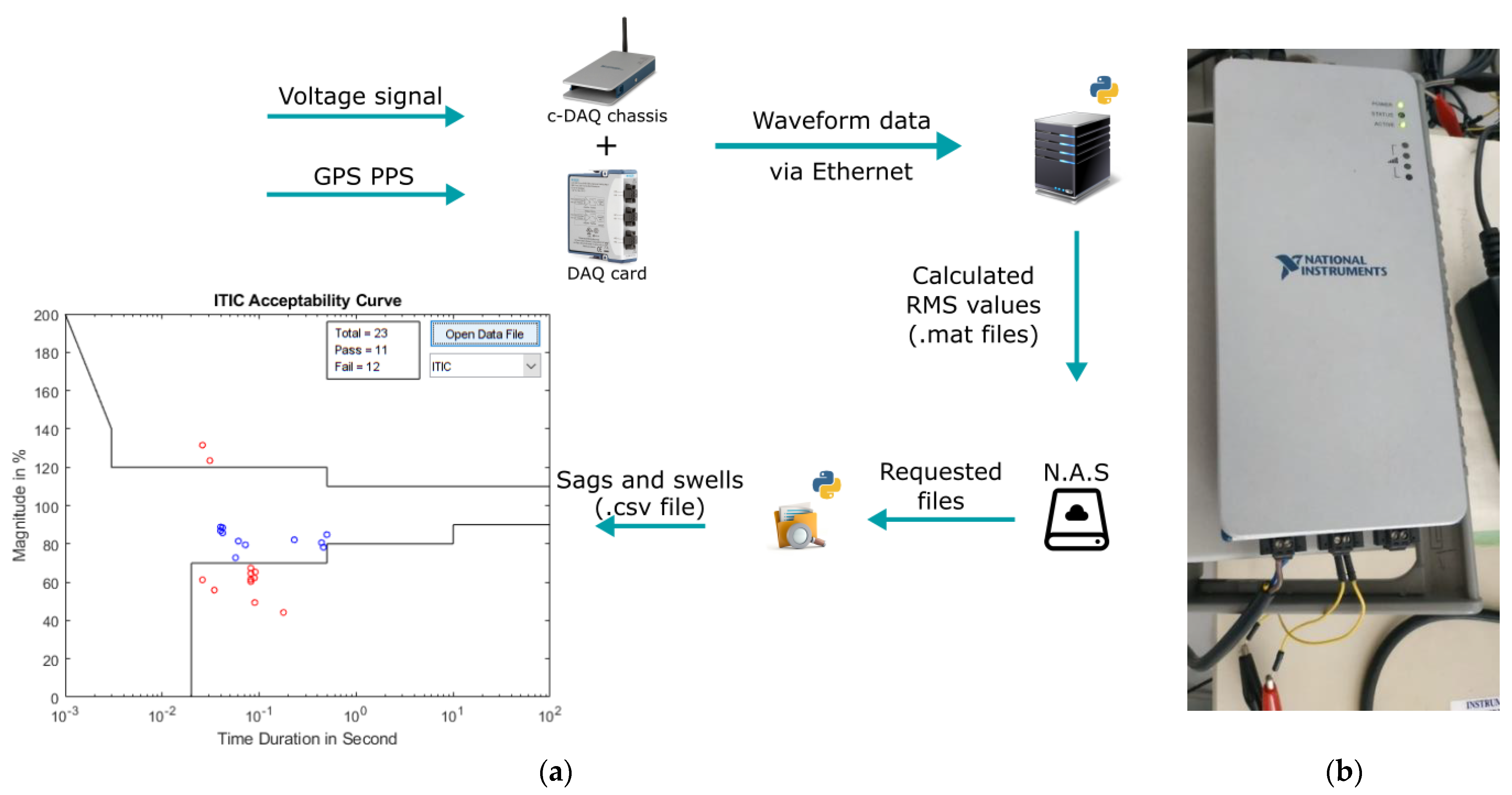
In order to study these phenomena, the first step is to set up a measurement chain to capture the voltage waveform and extract the data required for the analysis. The first two elements of the measurement chain are a data acquisition card (DAQ) and a c-DAQ chassis that contained the card (see
Figure 1). Both elements are manufactured by NI
TM. They receive, on the one hand, the voltage input taken directly from a wall socket and, on the other hand, a pulsed signal (1 PPS) from a GPS receiver, which provides the time stamp to the measures.
As explained in [
14], where the measurement chain of the system that monitors the electrical network and the different analyses carried out are detailed, the PPS signal is used to corroborate the time base of the acquisition card. The RMS voltage is calculated every single cycle of 50 Hz; therefore, between two PPS (1 s) there must be 50 RMS values. In this way, the PPS signal is used to verify that the sampling rate is correct and, therefore, the time of 20 ms between each RMS measurement is real.
Once both signals are connected to the chassis, the resulting data are transferred via Ethernet to a server running on Python.
On the server, the acquisition process is completed, and then voltage waveform data are available on the PC. Files are created every second to store data about the signal, and the fundamental ones are the instantaneous voltage in volts and the time mark that corresponds to each measurement. The sampling rate is 50 kSa/s, so each file has 50 k of voltage data. Taking this into account, 86,400 files and therefore 4,320,000 data are generated every day.
This sequence has been running continuously since its implementation; this gives an idea of the big volume of data that are continuously generated and stored. In this case, the files are saved in a Network Attached Storage (NAS).
In parallel, these raw signal data undergo numerous analyses in another
Python program. Multiple parameters such as frequency, RMS voltage, variance, higher order statistics (HOS), etc., are calculated, which aim to characterise the waveform. The results of these analyses are also saved every second in a database, which continues to increase the volume of data stored. Of these parameters, the one that will be used to search for voltage sags and swells is the RMS voltage, calculated using Equation (1).
where
N is the number of samples per cycle, and
n is the sample index. In the present case, the sampling rate was 50 kSa/s, and
VRMS was calculated every cycle of 50 Hz (every 20 ms), so 50 RMS values were available every 1 s. To organise the infinity of files generated every second (both for the instantaneous signal data and for the respective analyses performed), they are grouped into folders, dividing them by minutes, hours, days, months and years, following an ascending order.
Once these files are saved as described above, another Python program kicks in. This is responsible for the detection of voltage sags and swells in the stored files. To carry out this search, the first step is to establish the nominal RMS voltage and define the range from which the values are going to be considered as voltage sags/swells. Specifically, values above or below 10% of the nominal value for a duration of 1 cycle to 1 min were considered anomalous.
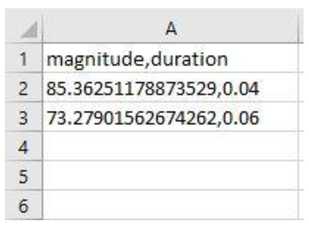
This program continuously tracks the RMS data, looking for outliers. In the case of consecutive out-of-range data, measurements are selected, and an average of their magnitude and the total duration of the sag or swell are calculated. When detected, the magnitude and duration of the different sags and swells are stored in .csv files that are created monthly. These files are available in the dataset and are used by the MATLAB function described below. As can be seen, all the acquisition, management and power quality analysis are programmed in
Python. In recent years, applications have emerged that use
Python as a programming language applied to the acquisition of supply voltage signals, such as [
15]. However, none of them use a model combined with MATLAB to plot the ITIC curve or any other means of visual representation of supply reliability zones.
For the representation of voltage sags and swells, a function similar to one developed by Aggiag et al. in [
16] was used, which allows plotting data pairs, indicating the magnitude and duration of the disturbance. This function, when executed, allows choosing any of the mentioned .csv files to represent the sags or swells within the implemented acceptability curves (ITIC, SEMI F47, IEC 61000-4-11 and Samsung). In this way, depending on the region of the curve in which each disturbance is located, the function itself dictates which disturbance is in the safety zone and which disturbances poses a risk.
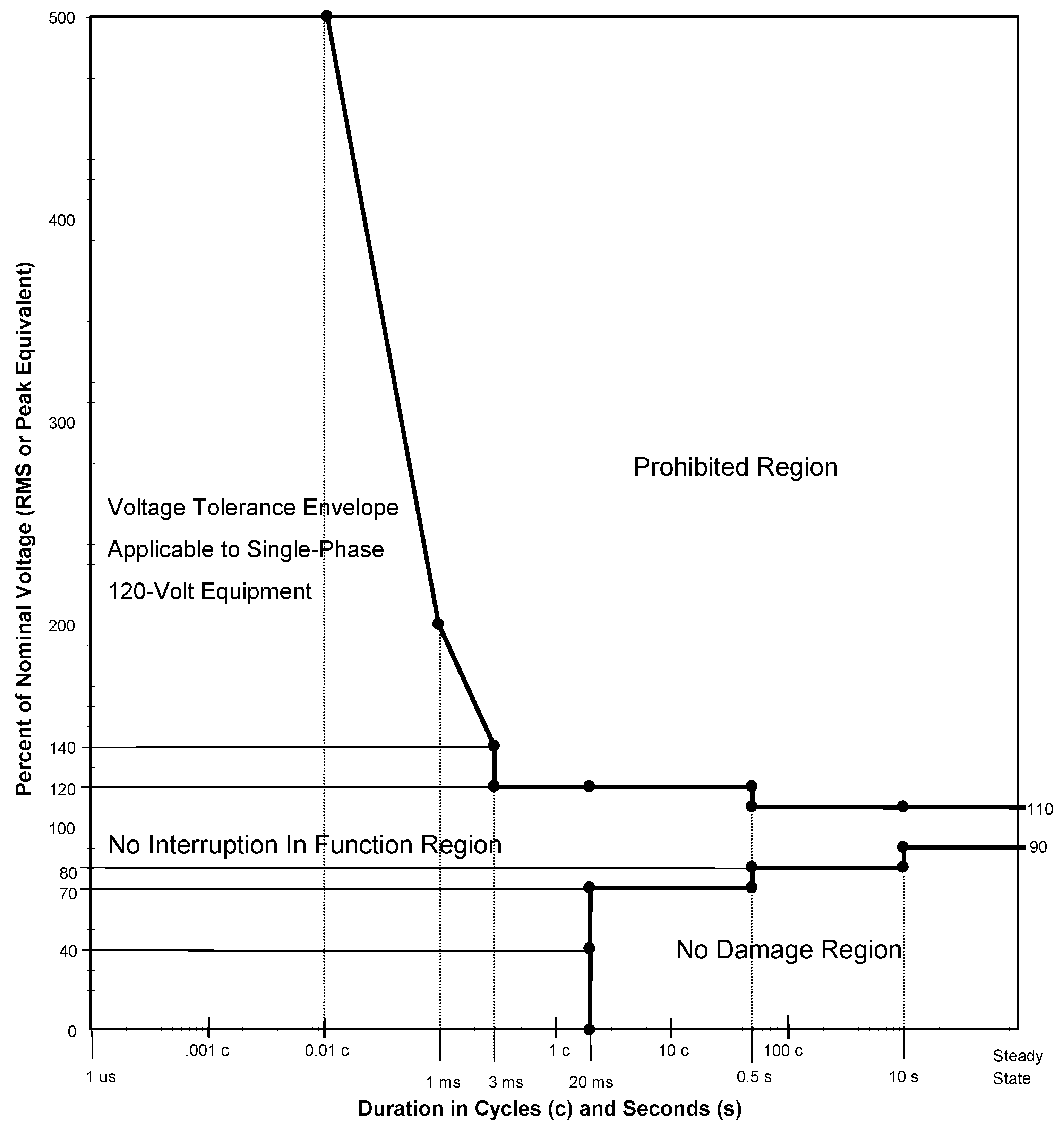
Among all acceptance curves, this paper focuses on the ITIC curve. This curve describes an AC input voltage envelope that can normally be tolerated (without interruption of operation) by most Information Technology Equipment (ITE) [
17].
Three main regions are distinguished on this curve: the region of operation without interruption (safety zone), the undamaged operation region (below the lower limit of the safety zone) and the prohibited region, above the upper limit of the safety zone, as seen in
Figure 2.
The “prohibited region” contains swells that exceed the upper limit of the curve; therefore, if the equipment is subjected to them, it is expected to fail. The “no damage region” includes voltage sags and interruptions that are more severe than those allowed in the safety zone, but which theoretically should not cause major damage to the equipment.
However, in a previous study [
18], the authors tested the effect of voltage sags on single-phase industrial robots and were able to verify that there are states that lead to receiver damage in an area they called “A” within the “no damage region” shown in
Figure 2. Those disturbances damaged the controller.
The main function of the ITIC curve is to protect equipment sensitive to voltage variations and to prevent the load centre from disconnecting due to the activation of protections that exhibit voltage disturbances. This is also subject to fines towards the load centre for improper disconnection. It also prevents damage to equipment sensitive to voltage variations.
4. Results
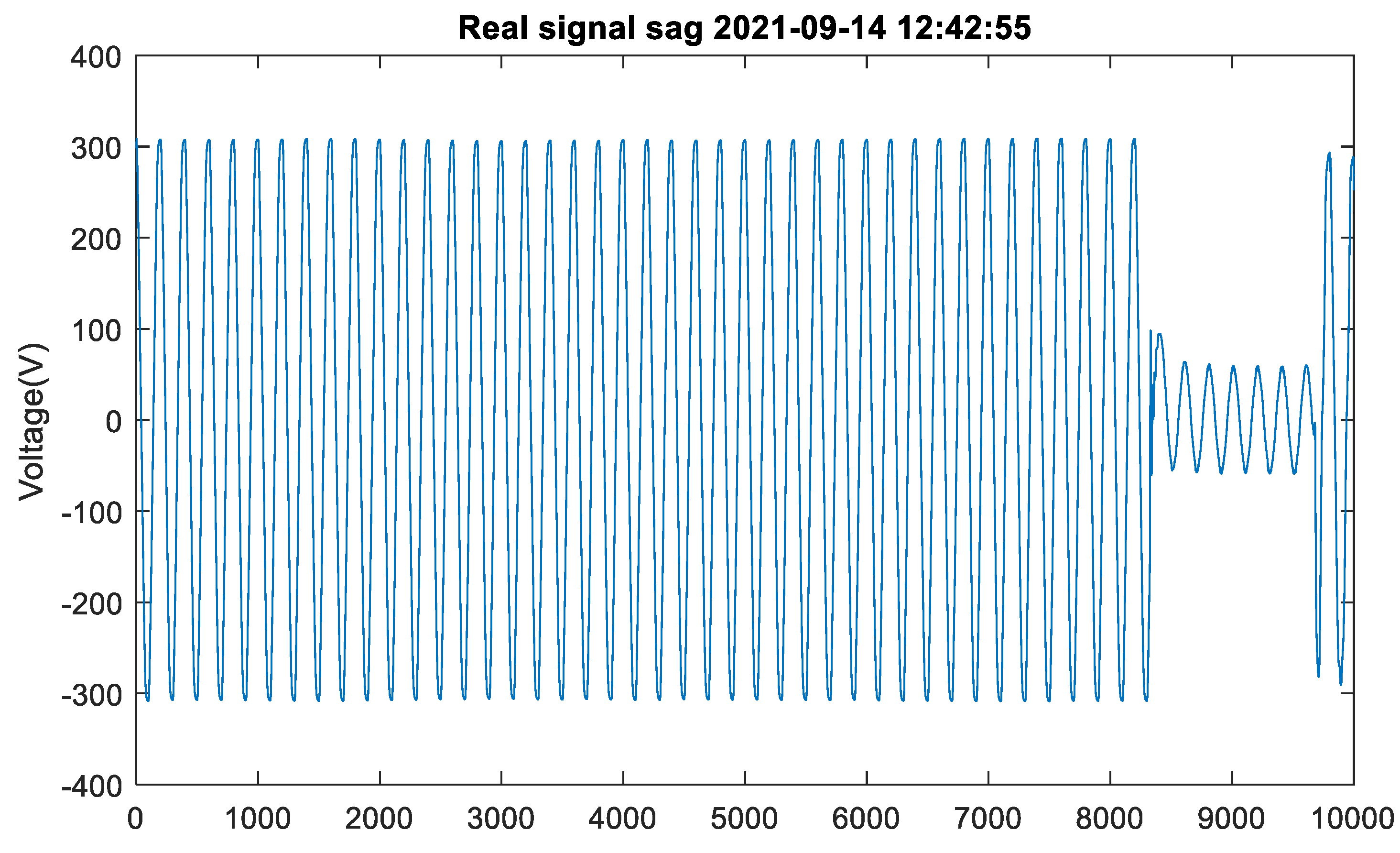
As explained in the previous section, to find voltage swells and sags, the RMS values resulting from the calculations performed by the server were used. However, instantaneous voltage data were also available on the PC. These data were acquired at a sampling rate of 10 kSa/s, and were stored in files created every second. These files can be useful for multiple purposes, which are not the focus of this article. One of the uses of instantaneous voltage data can be to visually detect voltage sags and swells directly from the original signal, which is especially useful when the duration of the failure is less than one cycle.
Using RMS voltage data resulting from the analysis performed by the server, the same sag observed in
Figure 4 could be corroborated in
Figure 5.
To search for voltage sags and swells, it was programmed a code written in Python that opened all the files dating within the specified time interval and detected those values above (swells) or below (sags) 10% of the nominal value. The magnitude in % of the nominal voltage and the duration of the disturbances were saved in .csv files.
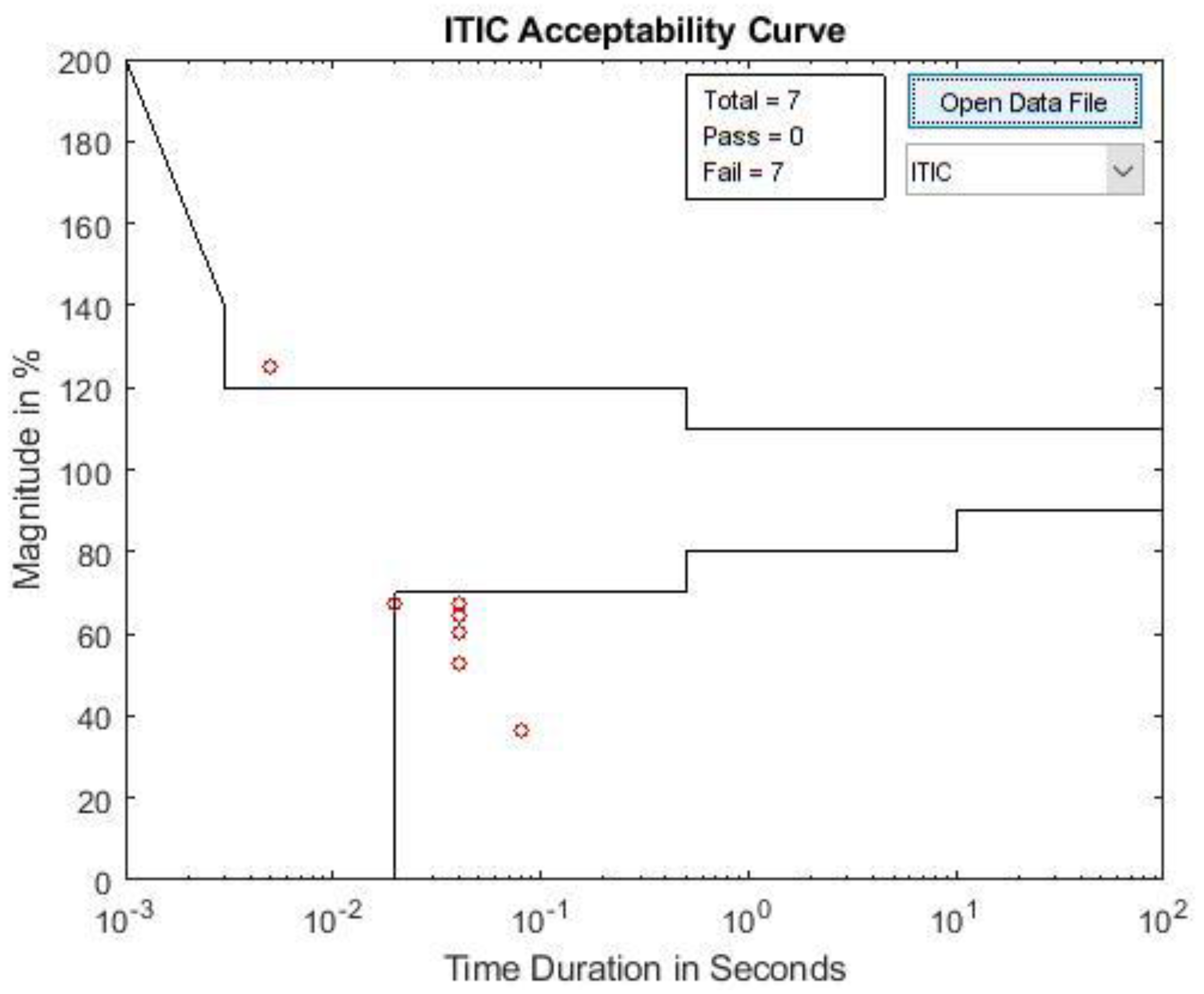
These files were then used to plot the detected voltage sags and swells on the acceptance curves using the MATLAB program. For example, the disturbances found in September 2021 are presented in
Table 1.
Representing the previous data on the ITIC curve, what can be seen in
Figure 6 was obtained:
Six voltage sags were detected this month, most of which occurred on 9 September. The magnitude and duration of all these sags exceeded the safety zone established by the ITIC curve, as shown in
Figure 6. A swell took place also on 21 September. Although its duration was quite short (5 ms), its magnitude (125%) was enough for the swell to be dangerous according to the acceptance curve that was used to analyse sags and swells.
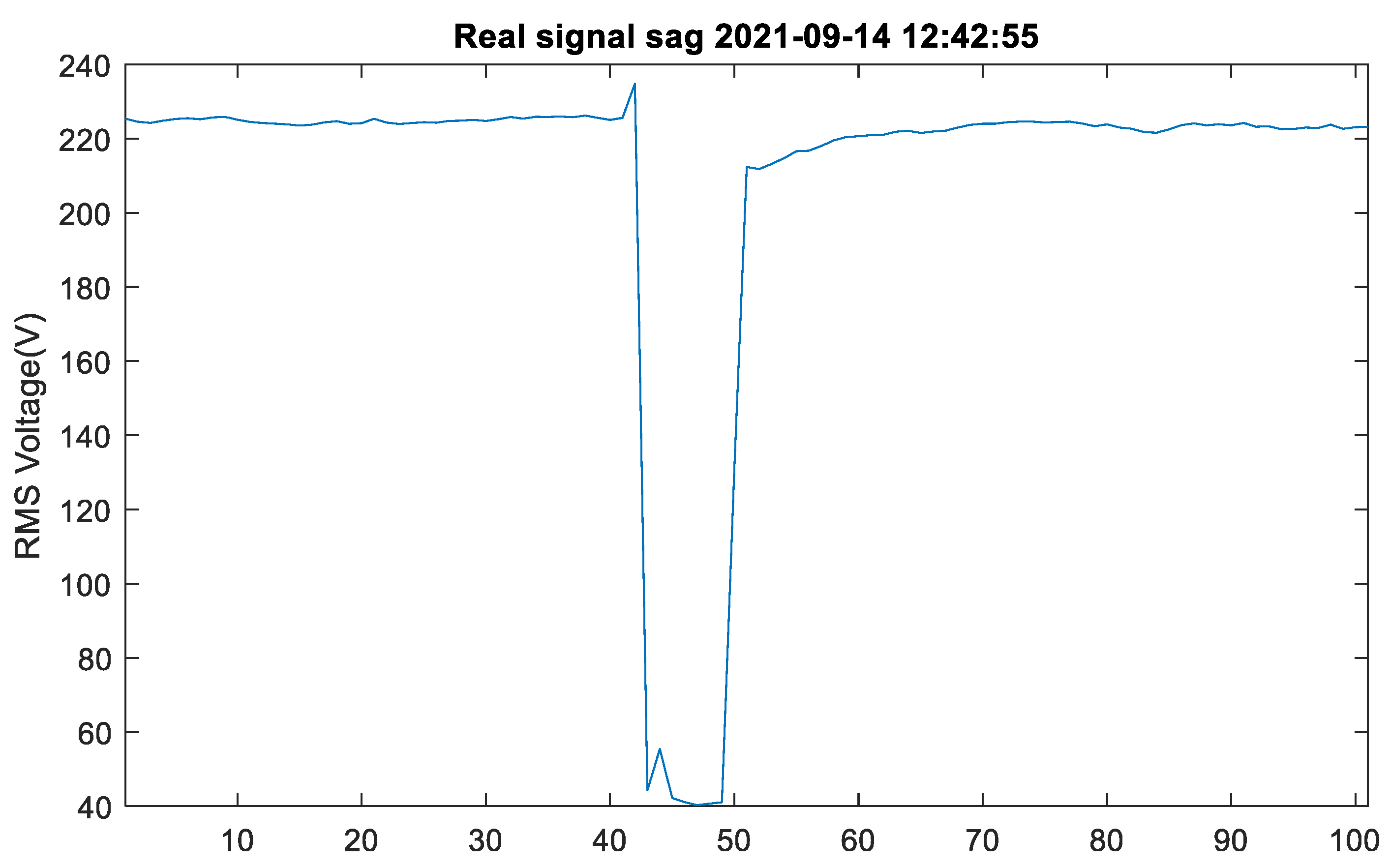
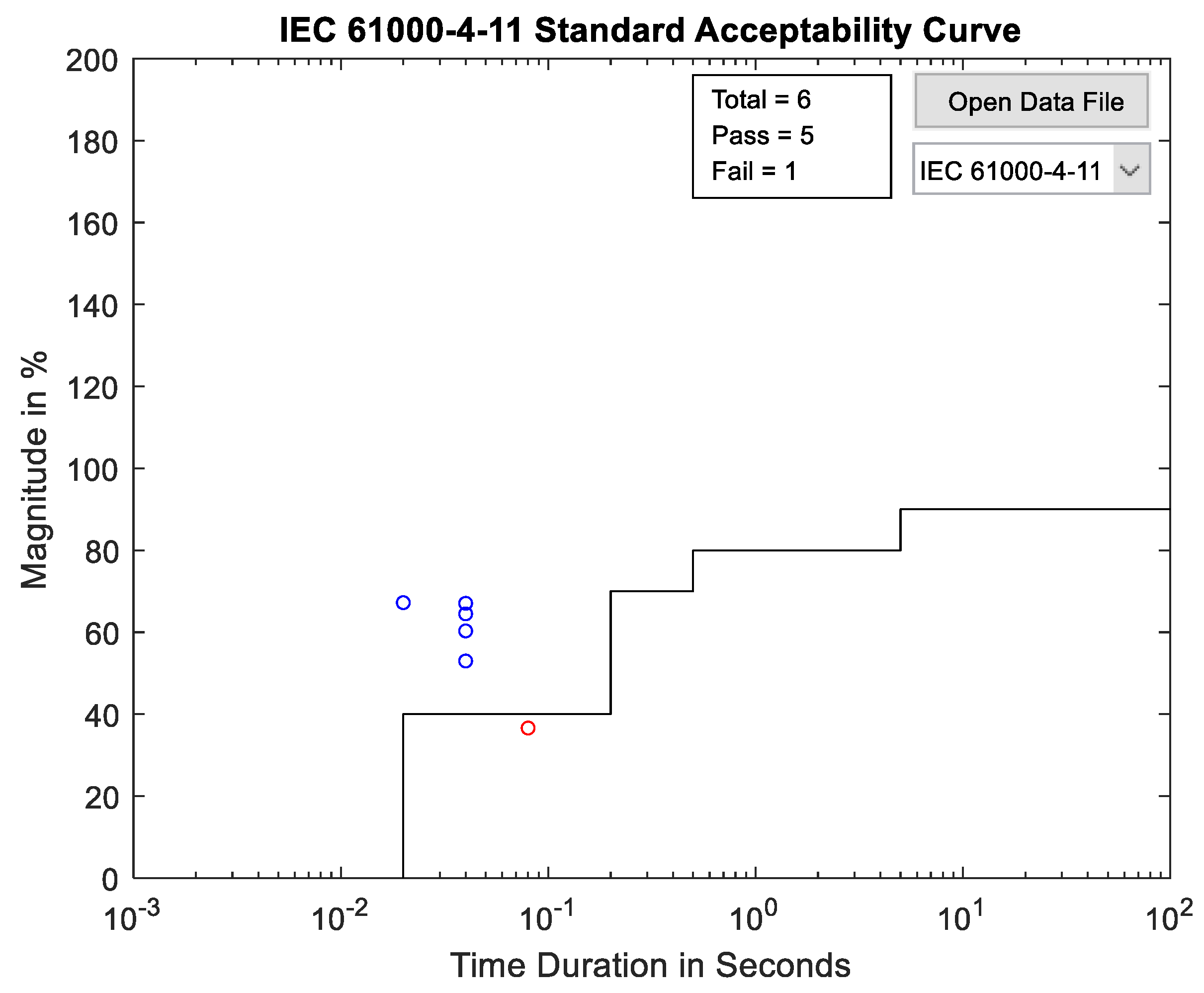
The most unfavourable sag occurred on 14 September, lasting 80 ms, in which the RMS voltage dropped to 36.62% of its nominal value. It was such an unfavourable sag that even in other more permissive curves, such as IEC 61000-4-11, it fell outside the safety zone, as shown in
Figure 7. This means that if a voltage sag of this magnitude and duration occurs, the equipment will not function.
Although voltage sags are not supposed to cause damage to the equipment, as they only cause it to stop working, in the case of a large voltage variation such as this one, it would be necessary to pay attention to the performance of the equipment connected to that point after the fault occurs.
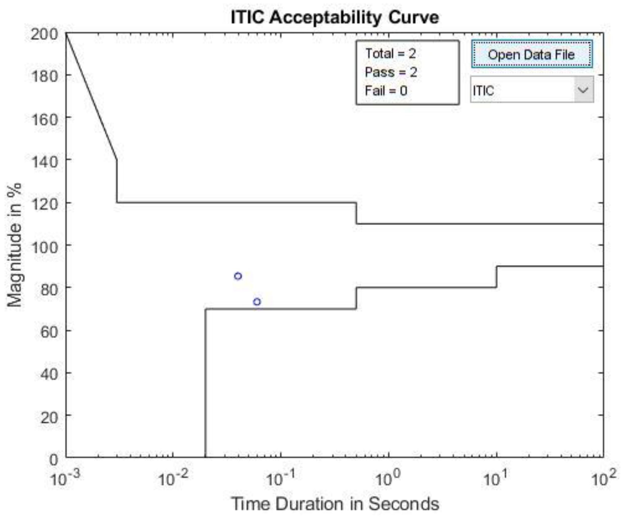
The case described above is unfavourable; in fact, in most of the months analysed, there were hardly any sags or swells, and if present, they were usually found in the safety area of the ITIC curve, as can be seen in
Figure 8.
No swell was detected in this month, and the sags detected had a permissible magnitude and duration, so that they were located in the safety zone of the curve. This is a sign that the power supply in terms of voltage level was fairly stable at the studied point of the network.


 ,
, 


