1. Summary
Surface freshwater mapping at different temporal (e.g., single or multiple time periods) and spatial scales (e.g., local to global) provides key baseline information to better understand human activities that both benefit from (e.g., ecosystem services), and that impact (e.g., impoundment) these ecosystems. Given the wealth of long-term continuous spaceborne Earth observation systems (e.g., Landsat series, Copernicus, PlanetScope, etc.) in orbit, satellite imagery has been the preferred method to map surface freshwater over large geographical areas (e.g., [
1,
2,
3]). For example, Ref. [
1] generated a 30 m pixel size global water cover dataset for 2000 and 2010 from Landsat TM/ETM+ and HJ-1 satellite imagery through a combination of pixel-based (spectral) and object-based analysis. Other global data sets such as ESA’s Land Cover CCI [
4] include water as one of the multi-temporal land cover classes, but the output is provided at a pixel size of 300 m. Recently, Ref. [
3] produced a global surface water cover dataset using the Landsat top-of-the-atmosphere reflectance archives for the period of March 1984–Oct 2015 with Google Earth Engine. The classification was based on an expert system taking into account the multi-temporal and multispectral aspects of the imagery producing surfaces of water occurrence, maximum extent, seasonality, recurrence, and transitions. A recently updated version includes data up to the year 2020 [
5]. However, as shown by [
6,
7] the high discrepancy between freely available freshwater datasets and in some cases inaccuracy, presents a challenge when determining which dataset to choose for specific applications. Additionally, large-extent fine spatial scale datasets such as the 2.5 million square kilometer riverscape classification at 2.5 m spatial resolution for Europe [
8] do not yet exist for South American rivers.
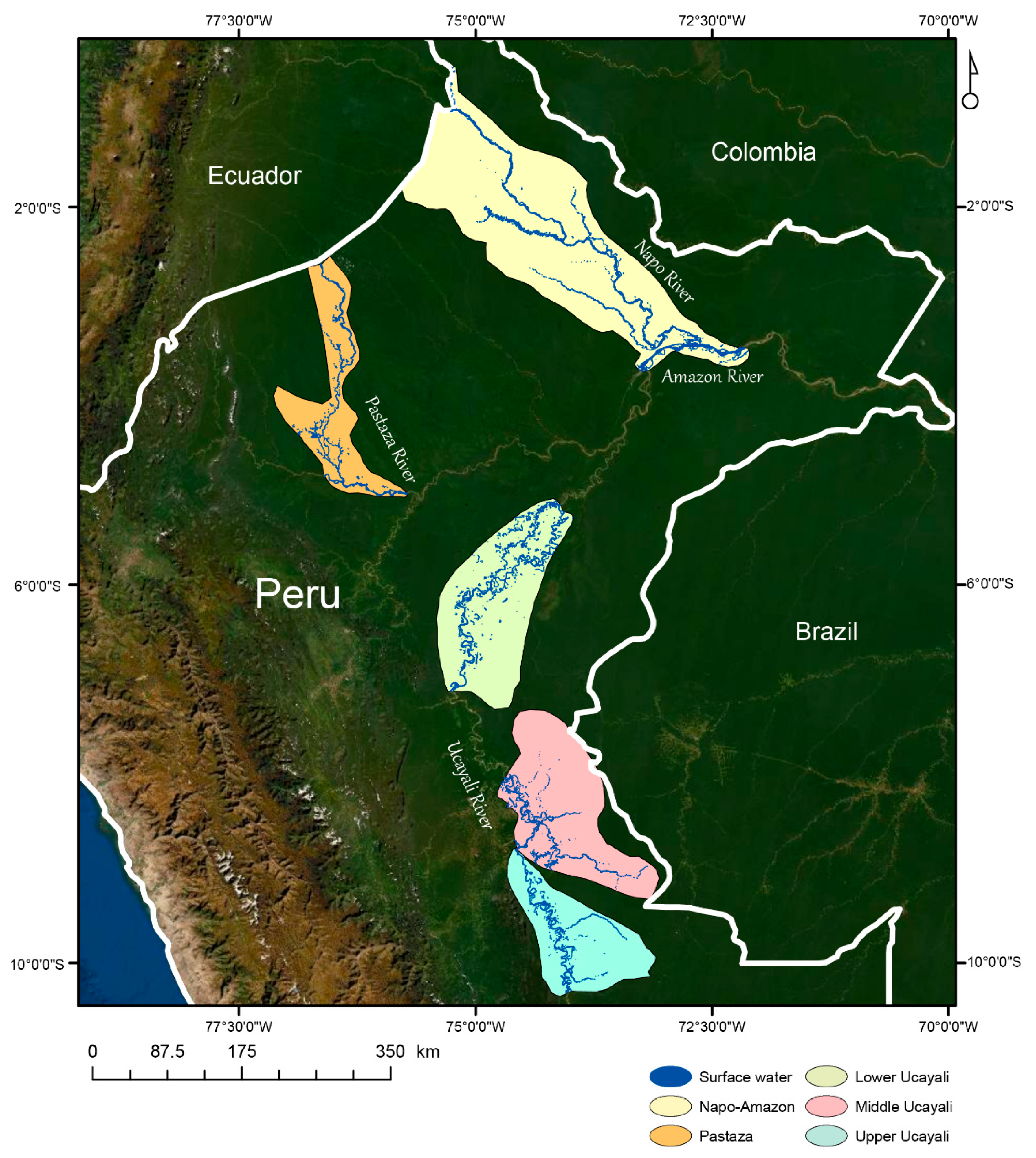
The Peruvian Amazon Rural Livelihoods and Poverty (PARLAP) Project [
9] is an effort aiming to better understand the nexus between livelihoods (e.g., fishing, agriculture, forest use, trade), poverty, and conservation in the Peruvian Amazon over a 35,000 km river network (Napo, Amazon, Pastaza and Ucayali basins) [
10]. River basins were selected to reflect heterogeneity in environmental conditions, economic activities, history, and indigeneity of its peoples. In the absence of roads, settlements are concentrated along rivers, and river reaches in each basin were the focus of community and household surveys. The character of surface water around communities is a key environmental feature, specifically of primary and non-main river features (e.g., oxbow lakes), which can be indicative of the available habitat for fish and other aquatic species along the active channel and floodplain, respectively.
Here we developed a minimum extent persistent surface water classification along reaches of the four major rivers (i.e., Amazon, Napo, Pastaza, and Ucayali) investigated by the PARLAP project, using Landsat satellite imagery with a 30 m pixel size, representing circa 1989, 2000, and 2015. Different from other surface water classification methodologies, we implemented a hierarchical ruleset predominantly based on a modified Normalized Difference Water Index (mNDWI) and shortwave infrared surface reflectance. Surface reflectance in the blue band and brightness temperature (BT) were included to minimize misclassification. Importantly, we differentiate between primary (i.e., main) and non-main channel water, this distinction is not available from any of the freely available datasets. Therefore, our surface water layers are distinct from other classifications and are part of PARLAP’s effort to better establish the link between livelihoods and this vast riverscape.
3. Methods
The surface water classifications were created for three time periods representing circa 1989, 2000, and 2015 from Landsat (TM 5, 7 ETM+, and 8 OLI respectively) satellite imagery at a 30 m pixel size for reaches of four rivers of interest in the Peruvian Amazon (i.e., Napo, Amazon, Pastaza, Ucayali). The circa 1989 data correspond to the earliest time for which imagery was available for the entire study area. The circa 2015 data correspond to when PARLAP carried out large-scale community and household surveys in the study area (2014–2016), and circa 2000 an intermediate period in-between. Due to the overall length of time (30 years), imagery from multiple satellites was necessary. Landsat TM 5 was in operation from March 1984–June 2013 [
12], Landsat 7 ETM+ has been in operation since April 1999 but suffered a Scan Line Corrector failure in June 2003 [
13], and Landsat 8 has been in operation since February 2013 [
14]. For practical purposes and for relating to other PARLAP field data, these surface water layers are organized into the five regions as shown in
Figure 1. The combined area across the river basins examined here is 113,691 km
2.
The classifications were carried out in Google Earth Engine using the USGS Landsat Surface Reflectance Tier 1 imagery collection [
15]. As commonly seen in the tropics [
16], the study area is prone to extensive cloud clover. The pixel QA bands were used to mask out clouds in order to generate a median surface reflectance product for each period. The QA bands are available as one of the metadata bands produced during standard Landsat processing and represent the pixel quality attributes generated from the CFMASK algorithm [
17]. The median reflectance composites represent the 1985–1989, 1999–2000, and 2014–2015 periods. The differences in the length of time are the minimum number of years needed to generate a cloud-free composite for the entire study area.
Table 1,
Table 2 and
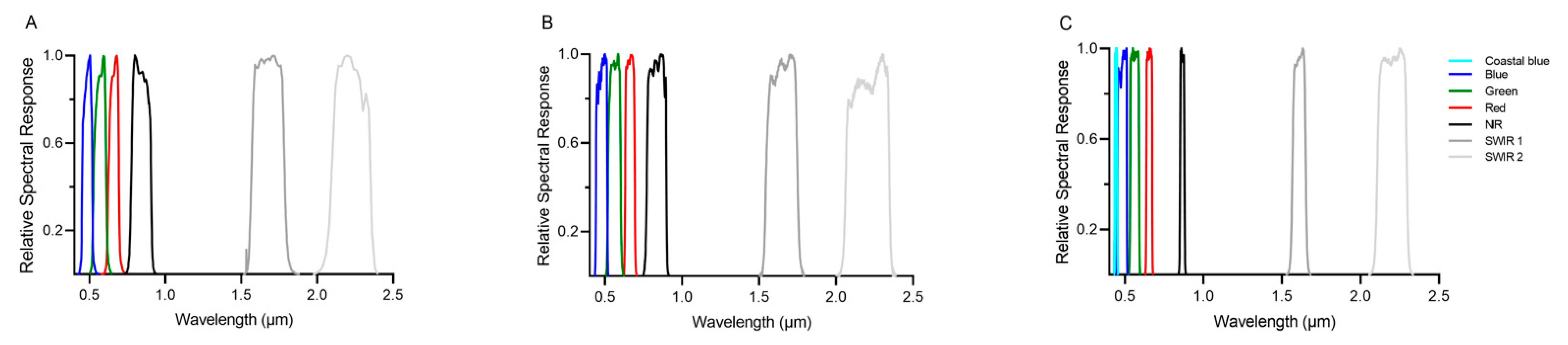
Table 3 describe the optical and thermal bands from the three Landsat satellites.
Figure 3 illustrates the relative spectral responses of the optical bands. Importantly, as surface reflectance products, the images had undergone an atmospheric compensation to remove the effects of the atmosphere (e.g., scattering, absorption).
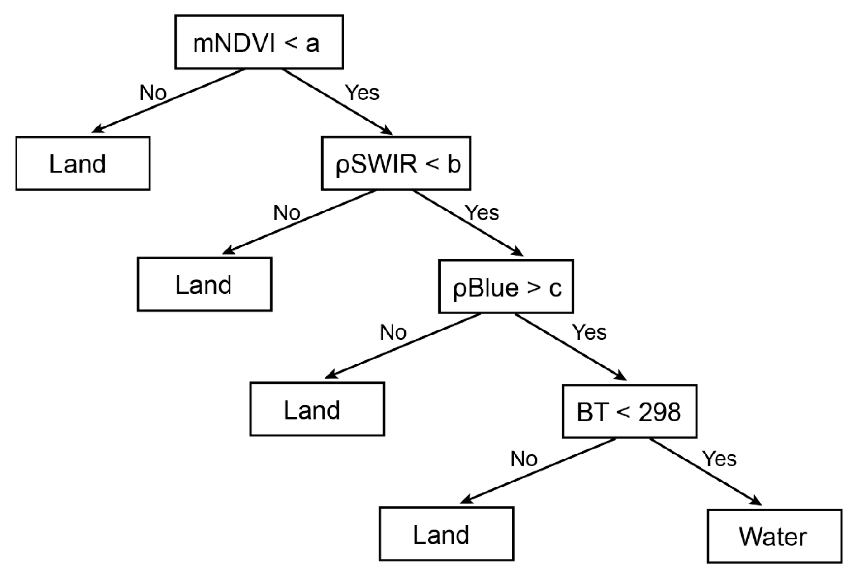
Classification was based on a hierarchical, binary logical ruleset that took into consideration surface reflectance, and brightness temperature (BT). Our final products represent the minimum extent of persistent surface water. Each component of the ruleset is described below.
3.1. Surface Reflectance
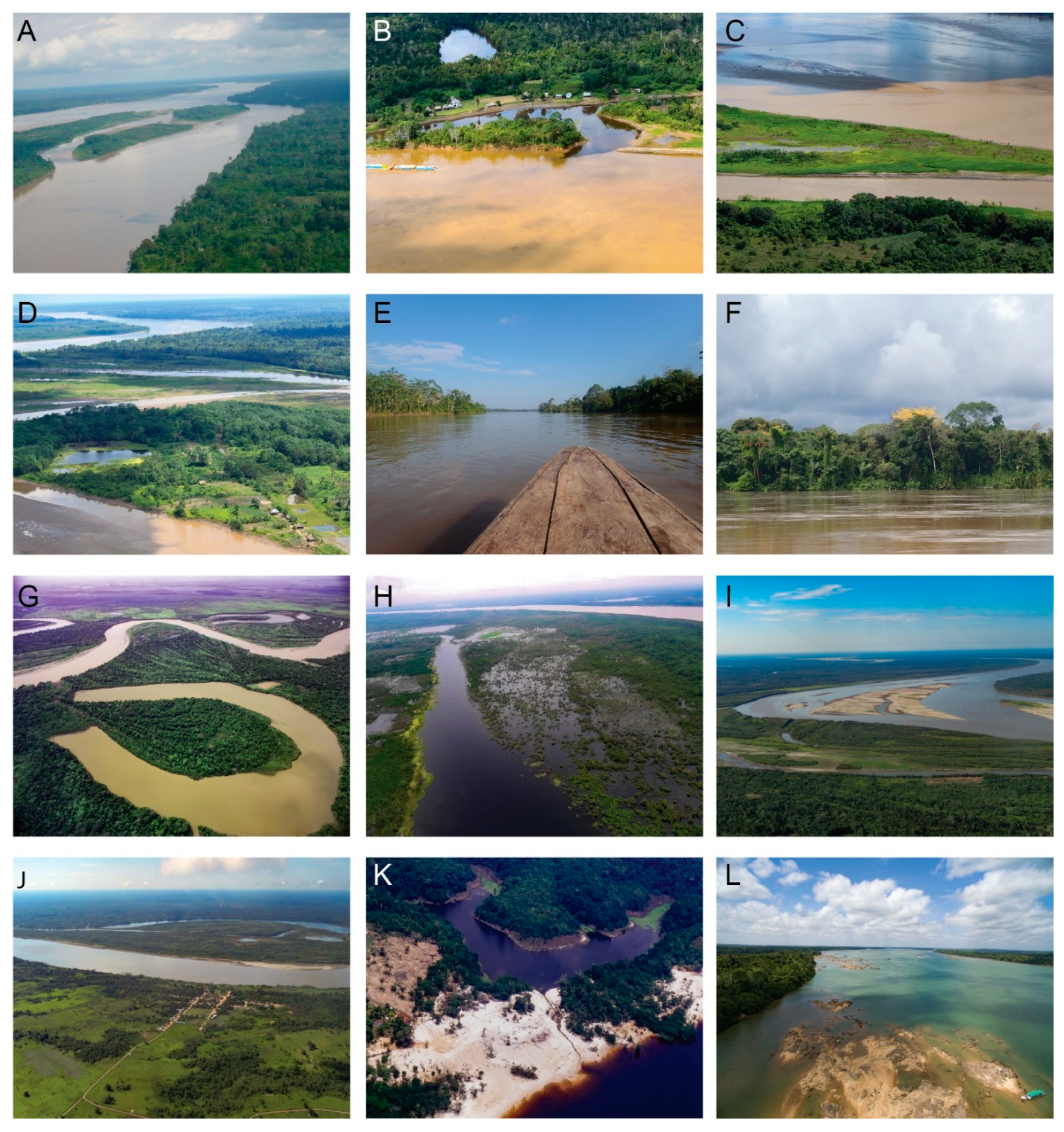
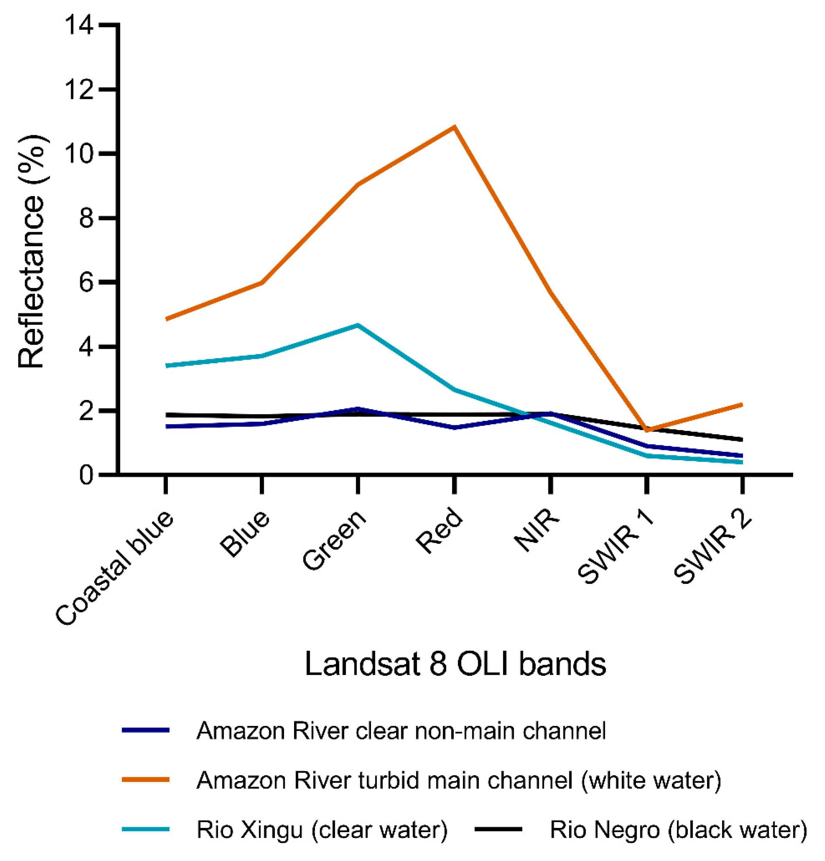
Unlike many other large bodies of freshwater such as the African and North American Great Lakes, or clearwater and blackwater tributaries of the Amazon such as the Rio Xingu, and Rio Negro, respectively, the main channels of the rivers mapped in this dataset are considered whitewater rivers. An important characteristic of whitewater rivers is the high sediment load (see
Figure 2) which impacts the surface reflectance (
Figure 4 and
Figure 5). Water is known to be a low signal target, absorbing most of the solar irradiance across wavelengths. High sediment loads increase reflectance in the visible and near-infrared (NIR) bands which can lead to confusion with some terrestrial land covers. Across the surface water in the study area, a range of turbidities can be seen, from relatively clear, small lakes to the high sediment-laden main channels.
For open water delineation, the original formulation of NDWI [
20] was developed as Equation (1):
where ρ denotes surface reflectance.
Other previous formulations of NDWI (e.g., [
21]) using a NIR and SWIR band instead were developed for assessing water content in plant canopies or as defined by [
22] replace the NIR band with a SWIR band in Equation (1) for open water mapping.
In order to account for the range of turbidities encountered in the study area (
Figure 4), a modified Normalized Difference Water Index (mNDWI) based on [
20] was calculated from the green, red, and NIR bands according to Equation (2):
where ρ is the surface reflectance in the NIR, red, or green bands of the respective sensors (
Figure 3). The value of 100 is a scaling factor. The mNDWI from Equation (2) is the first level in the hierarchical ruleset (see
Section 3.3).
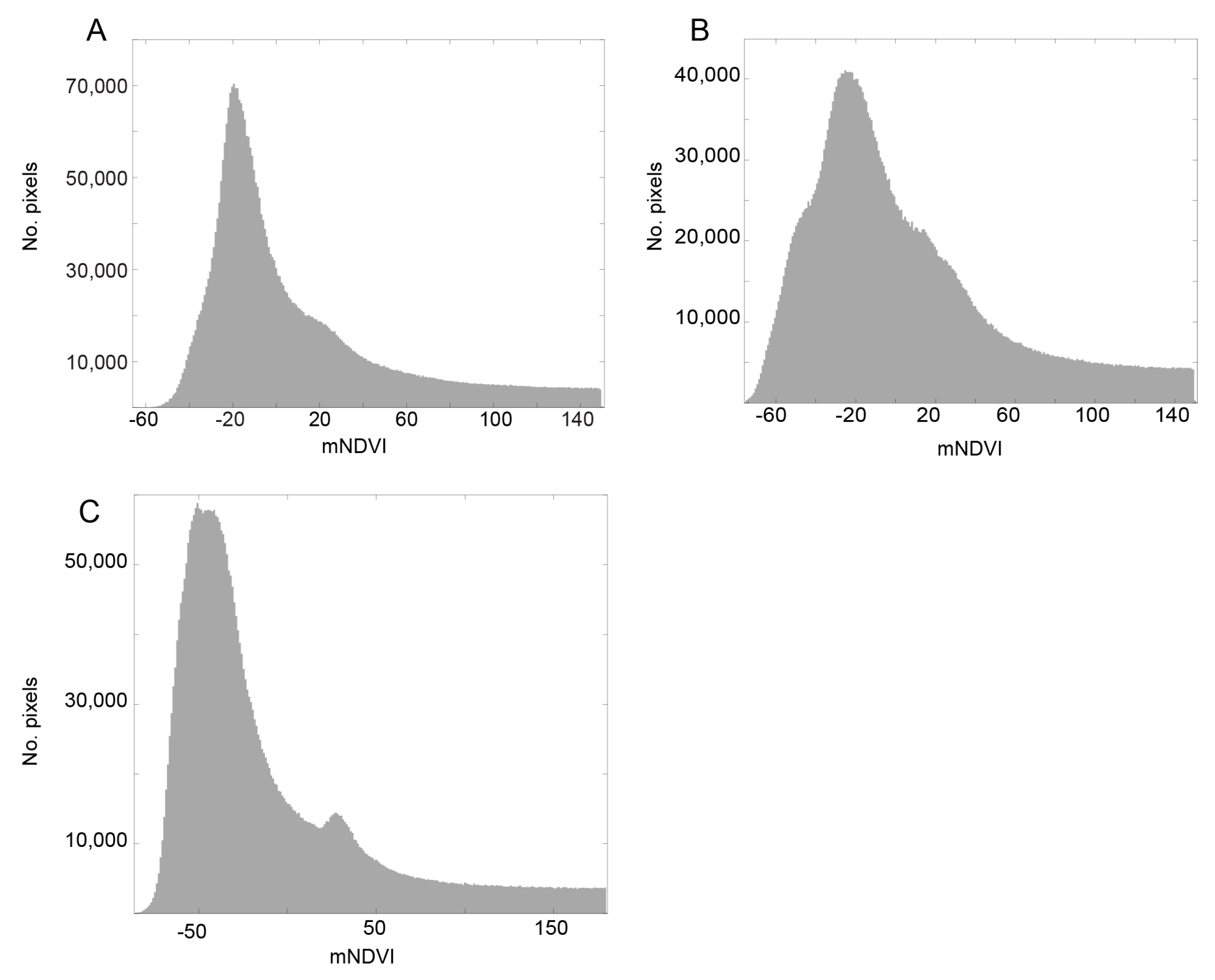
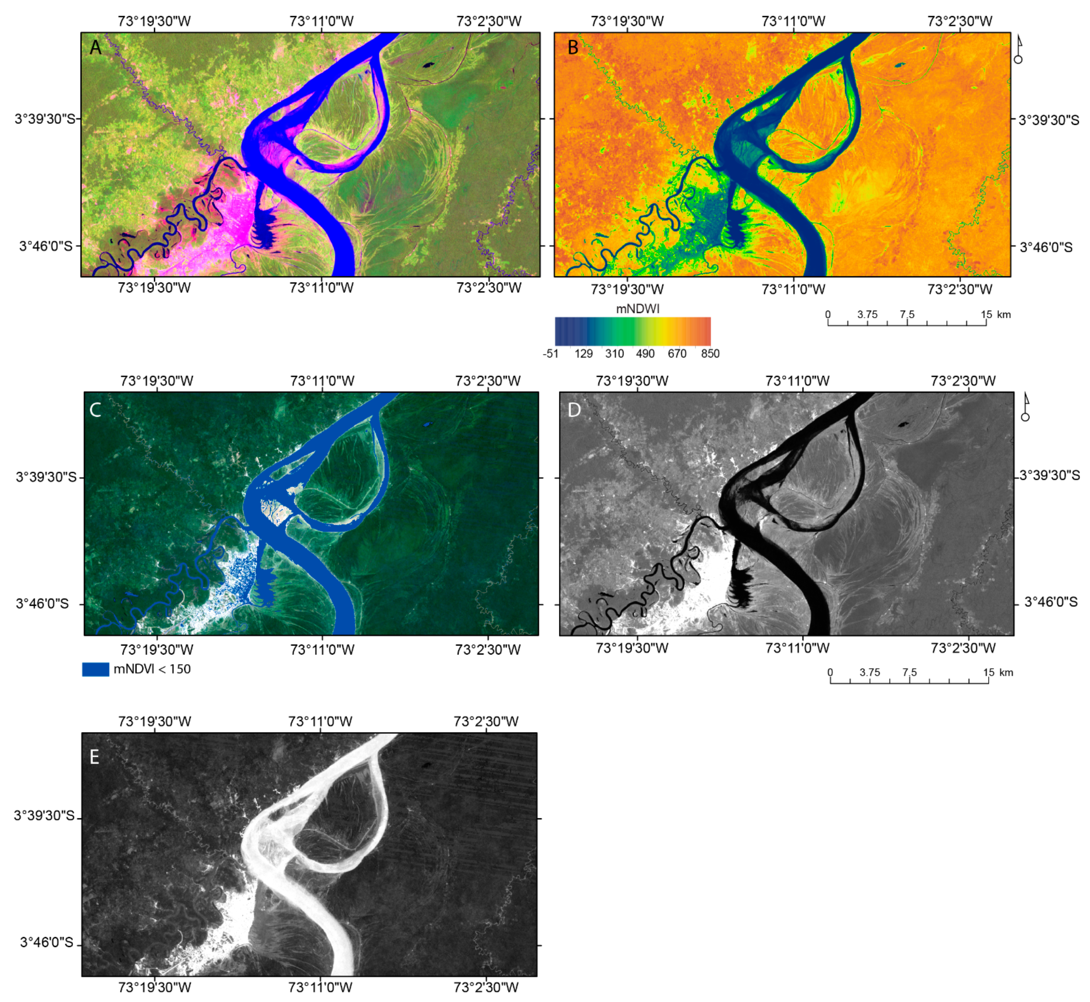
In our ruleset, the threshold of mNDWI from Equation (2) varied by time period. For example, for the earliest period from TM 5 (circa 1989) the mNDWI threshold was set to <150 (
Figure 5 and
Figure 6,
Table 4).
To refine the separation of open water from other land cover classes, the next level in the hierarchical ruleset was a threshold of SWIR2 reflectance (
Table 1). As seen in
Figure 5, in order to include the less turbid non-main channel features, the relatively higher threshold of mNDVI also results in the inclusion of pixels representing larger settlements such as Iquitos, but the reflectance of the urban areas and water are considerably different in the SWIR2 band (
Figure 5). The third level of the hierarchical ruleset is the reflectance in the blue band. Water is higher reflectance than the surrounding vegetation in the blue band (
Figure 5), therefore this threshold refined the edges of the detected surface water and eliminated misclassifications due to topographic shadows.
3.2. Brightness Temperature
The fourth level of the ruleset (predominantly for refinement) was brightness temperature (BT) from the thermal band of the images used in the surface reflectance mosaics. For Landsat TM 5 and 7 ETM+ this is band 6 (10.4–12.5 µm). Landsat 8 TIRS has two longwave infrared bands (bands 10 and 11); here we used band 10 (10.6–11.19 µm). While these longwave infrared (LWIR) bands were acquired at 120 m (TM 5), 60 m (7 ETM+), or 100 m (TIRS) pixel sizes, in the surface reflectance collections accessed through Google Earth Engine, they have been resampled to 30 m through cubic convolution [
15]. Brightness temperature considers an emissivity (ε) of 1 and represents the temperature a blackbody (i.e., theoretical perfect emitter and absorber of radiation) would be if observed at the same wavelength. Emissivity is a measure of the efficiency of a material to emit radiation in comparison to a blackbody and is a fundamental property of materials in the LWIR (i.e., thermal) region according to Kirchoff’s Law Equation (3):
where E is the total amount of energy emitted (i.e., flux density) by a material (per unit time, per unit area) at a specific temperature (T) and σ is the Stefan-Boltzmann constant (5.67 × 10
−8 W m
−2 K
−4). Emissivity is unitless ranging from 0–1, with values closer to 1 representing material more similar to a blackbody at the wavelength of observation. Materials differ in their ε values across wavelengths; liquid water generally has an ε > 0.97 with minimal effect of turbidity in the LWIR [
23,
24,
25,
26]. While LWIR energy emission is generally considered to be a surface property, in water bodies up to the top 100 µm may comprise the volume contributing to the emission [
25]. For the surface water classifications, the BT threshold was set to less than 298 K for all datasets. The majority of the urban pixels had a BT > 300 K.
3.3. Final Ruleset
The final hierarchical binary ruleset is shown in
Figure 7 where a-c are the time period specific thresholds for each term (see
Table 4):
3.4. Generation of Vector Datasets
The binary surface water classifications were exported as images in GeoTiff format from Google Earth Engine and converted to a vector (polygons) data type in ArcMap 10.5 (ESRI, Redlands, CA, USA) for clean-up. Polygons representing the non-main channel water were manually extracted into a separate shapefile and polygons were dissolved into a single aggregate polygon layer. For polygons that comprised the main channel, topological rules of Must Not Have Gaps and Must Not Overlap [
27] were applied. The main channel polygons were also dissolved into a single aggregate polygon layer.
3.5. Validation
Validation points were created in Google Earth Engine through visual interpretation of the corresponding cloud-free Landsat mosaics. A total of 445 water and 445 land points were generated for each of the three time periods across all basins. Edge pixels representing the boundaries between classes were avoided.
Table 5,
Table 6 and
Table 7 illustrate the confusion matrices for the three time periods. High accuracies were achieved for all time periods (>90%). The misclassifications result from points where the river is too narrow to have been included in the final classification.
5. Discussion and Conclusions
To improve upon our results, further research examining the potential of monthly or quarterly high spatial resolution basemap mosaics (3.7 m resolution) suitable for machine vision analysis, or surface reflectance mosaics from the Planet Dove constellation for recent (from 2016 onwards) time periods should be examined. These data would increase the number of small non-main channel water bodies and narrow creeks that could be resolved (e.g., [
28]). For example, Ref. [
29] showed a significant decrease in the Lake Powell reservoir surface area between 2019 and 2021 from PlanetScope imagery classified in Google Earth Engine on a bi-weekly basis. Such high temporal resolution data may also be beneficial in the Peruvian Amazon to track rapid changes during the inundation of the floodplain in the high water season. As shown by [
30], such imagery used in combination with in situ river gauge data, a semi-automated river flow estimation could be derived. Nevertheless, for long-term records of historical change (i.e., prior to the availability of high spatial resolution satellite imagery) in locations without aerial or satellite photography, moderate resolution satellite imagery continues to be a source of valuable information about changes in the landscape.


 ,
, 


