An Eddy Covariance Mesonet For Measuring Greenhouse Gas Fluxes in Coastal South Carolina

Abstract

Coastal ecosystems are vulnerable to climate change and have been identified as sources of uncertainty in the global carbon budget. Here we introduce a recently established mesonet of eddy covariance towers in South Carolina and describe the sensor arrays and data workflow used to produce three site-years of flux observations in coastal ecosystems. The tower sites represent tidal salt marsh (US-HB1), mature longleaf pine forest (US-HB2), and longleaf pine restoration (replanted clearcut; US-HB3). Coastal ecosystems remain less represented in climate studies despite their potential to sequester large amounts of carbon. Our goal in publishing this open access dataset is to contribute observations in understudied coastal ecosystems to facilitate synthesis and modeling analyses that advance carbon cycle science.

Data Set:

https://doi.org/10.17190/AMF/1660341 (US-HB1)

https://doi.org/10.17190/AMF/1660342 (US-HB2)

https://doi.org/10.17190/AMF/1660343 (US-HB3)

Data Set License: AmeriFlux Data Use Policy; CC-BY-4.0

1. Summary

Terrestrial ecosystems are important components of Earth’s carbon cycle as they currently offset approximately 37% of anthropogenic fossil fuel emissions [1]. The strength of the terrestrial carbon sink varies from year to year, and while the mechanisms controlling this variability are not completely understood, land management activities, climate variability, and disturbances are major regulators of large scale carbon fluxes [2]. Therefore it is important to increase mechanistic understanding of terrestrial carbon cycling to improve the ability to predict future changes to the carbon sink in response to global environmental change. This importance has led to an increased demand for observations of atmospheric carbon dioxide concentrations and related surface fluxes [3,4,5] with an accompanying call to make access to these data more open and user-friendly [6].

Within coastal ecosystems, at the margins of terrestrial ecosystems, are tidal wetlands or so called “blue carbon” ecosystems, which have been identified as particular sources of uncertainty in the global carbon budget [7,8]. There is considerable interest in improving inventories and understanding of carbon sequestration in coastal ecosystems due to their potential to sequester large quantities of carbon, buffer coasts from storms, provide essential fish habitat, and improve water quality [9,10,11]. The southeastern United States is somewhat unique in that the extensive blue carbon ecosystems of the Gulf and Atlantic Coasts are bordered by highly-productive upland forested ecosystems that, combined, contribute a substantial portion of national terrestrial carbon sequestration [12]. Much of that carbon sink is provided by rapidly-growing southern pine trees, including important commercial species such as loblolly pine (Pinus taeda), which has helped to earn the region’s nickname as the “wood basket of the United States” [13,14,15]. A number of environmental and climate factors are thought to influence forest carbon sequestration rates, including stand age, successional stage, local precipitation and temperature, and land-use history, though knowledge gaps remain [16].

While loblolly pine’s expansion as a commercial species has had economic benefits, when accompanied by agricultural expansion, other land use change, and anthropogenic fire suppression, it has contributed to a nearly 97% loss of longleaf pine’s (Pinus palustris) native range [17,18]. Since longleaf pine habitat is valued for its biodiversity, including for endangered species, as well as cultural and historic value [19] there is substantial interest in restoring longleaf pine [20,21]. However its potential to sequester carbon and use water efficiently relative to other species is not fully understood [22]. Ultimately, while important progress has been made in measuring landscape scale water and carbon budgets in southeastern coastal plain pine forests [23,24,25,26] and tidal wetlands [27,28,29], much work remains to be done.

To that end, we have recently established a cluster of co-located eddy covariance towers in coastal South Carolina to measure the carbon, water, and energy fluxes between the land and atmosphere, as well as meteorological and phenological variables. The mesonet is designed to more thoroughly explore the mechanisms driving greenhouse gas exchange in coastal ecosystems that have received less attention from the flux community. US-HB1 was constructed in a blue carbon tidal wetland, US-HB2 is above a mature mixed pine stand, and US-HB3 is located in a longleaf pine habitat restoration site. We have two goals in describing and distributing our methods and data. First, we aim to describe the details of this new mesonet of towers and associated data workflow to ensure the resulting dataset is fully documented. Second, we are making this dataset openly and publicly available to be used by other investigators to help advance climate and carbon cycle science.

The eddy covariance method is currently the most accurate approach available to measure gas exchanges integrated over a specific area [30]. It achieves this through statistical analyses of a combination of (in situ) high frequency gas mixing ratio and wind velocity measurements. Though it was once a specialized technique used by micrometeorologists, innovative technological, methodological, and computational advances have broadened its use in other branches of science and industry including ecology, agriculture, and industrial regulation [31]. Yet barriers remain to an even wider adoption of the eddy covariance method, including the complexity of the system design, implementation, and data processing procedures given the large volume of data necessary to complete the calculations [32]. In an effort to provide transparency regarding data collection in the new mesonet, this paper documents the sensors, data acquisition systems, data processing, and quality control framework that created three open access datasets.

2. Data Description

There are four phases for handling data from the mesonet: raw measurement collection, quality assurance and quality control, flux processing, and open data publishing/storage. This process results in a yearly final data product for each of the co-located tower sites, made available as an open AmeriFlux dataset including 12 months of carbon, water, and heat flux observations. The AmeriFlux network is a United States’ Department of Energy (DOE) Office of Biological and Environmental Research (BERS) funded Terrestrial Ecosystem Science (TES) program created to collect, store, distribute, and synthesize data from eddy covariance sites studying terrestrial carbon cycling in the Americas [33]. It supports operation of a core group of flux tower observation sites and also provides open data hosting and online data publishing services, allowing for other sites to contribute to the network. Data submitted to the network must follow AmeriFlux’s standardization guidelines and pass their data Quality Assurance/Quality Control (QA/QC) practices, which we have used in producing the datasets documented herein. Table 1 outlines the specifics of these datasets, including descriptions and units of measured variables. The data can be accessed through the mesonet’s site information pages for US-HB1, US-HB2, and US-HB3. Work flow details and a complete listing of the towers’ raw measured variables are included in the methods and supplementary sections.

Table 1. Complete list of columns in the AmeriFlux-formatted data product. Labels 1,2, or 3 correspond to measurement sites (US-HB1, US-HB2, US-HB3 respectively).

	Variable	Description	Units
TIMEKEEPING
	TIMESTAMP_START${}^{\mathit{123}}$	ISO timestamp start of averaging period	YYYYMMDDHHMM
	TIMESTAMP_END${}^{\mathit{123}}$	ISO timestamp end of averaging period	YYYYMMDDHHMM
BIOLOGICAL
	LEAF_WET${}^{\mathit{23}}$	Leaf wetness, range 0–100	%
FOOTPRINT
	FC_SSITC_TEST${}^{\mathit{123}}$	Foken et al 2004 Post Field Quality Control [34]	adimensional
	FETCH_70${}^{\mathit{123}}$	Distance at which footprint cumulative probability is 70%	m
	FETCH_80${}^{\mathit{123}}$	Distance at which footprint cumulative probability is 80%	m
	FETCH_90${}^{\mathit{123}}$	Distance at which footprint cumulative probability is 90%	m
	FETCH_MAX${}^{\mathit{123}}$	Distance at which footprint contribution is maximum	m
GASES
	CO${{}_2}^{\mathit{123}}$	Carbon Dioxide (CO${}_2$) mole fraction in wet air	$\mu$molCO${}_2$ mol${}^{-1}$
	CO${}_2$_SIGMA${}^{\mathit{123}}$	Standard deviation of carbon dioxide mole fraction in wet air	$\mu$molCO${}_2$ mol${}^{-1}$
	FC${}^{\mathit{123}}$	Carbon Dioxide (CO${}_2$) turbulent flux (no storage correction)	$\mu$molCO${}_2$ m${}^{-2}$ s${}^{-1}$
	H${}_2$O${}^{\mathit{123}}$	Water (H${}_2$O) vapor mole fraction	mmolH${}_2$O mol${}^{-1}$
	H${}_2$O_SIGMA${}^{\mathit{123}}$	Standard deviation of water vapor mole fraction	mmolH${}_2$O mol${}^{-1}$
	SC${}^{\mathit{123}}$	CO${}_2$ storage flux	$\mu$molCO${}_2$ m${}^{-2}$ s${}^{-1}$
HEAT
	G${}^{\mathit{23}}$	Soil heat flux	W m${}^{-2}$
	H${}^{\mathit{123}}$	Sensible heat turbulent flux (no storage correction)	W m${}^{-2}$
	H_SSITC_TEST${}^{\mathit{123}}$	Foken et al 2004 Post Field Quality Control [34]	adimensional
	LE${}^{\mathit{123}}$	Latent heat turbulent flux (no storage correction)	W m${}^{-2}$
	LE_SSITC_TEST${}^{\mathit{123}}$	Foken et al 2004 Post Field Quality Control [34]	adimensional
	SH${}^{\mathit{123}}$	Heat storage flux in the air	W m${}^{-2}$
	SLE${}^{\mathit{123}}$	Latent heat storage flux	W m${}^{-2}$
ATMOSPHERE
	PA${}^{\mathit{123}}$	Atmospheric pressure	kPa
	RH${}^{\mathit{123}}$	Relative humidity, range 0–100	%
	T_SONIC${}^{\mathit{123}}$	Sonic temperature	${}^{\circ }$C
	T_SONIC_SIGMA${}^{\mathit{123}}$	Standard deviation of sonic temperature	${}^{\circ }$C
	TA${}^{\mathit{123}}$	Air temperature	${}^{\circ }$C
	VPD${}^{\mathit{123}}$	Vapor Pressure Deficit	hPa
PRECIPITATION
	P_RAIN${}^{\mathit{123}}$	Rainfall	mm
RADIATION
	ALB${}^{\mathit{123}}$	Albedo, range 0–100	%
	LW_IN${}^{\mathit{123}}$	Longwave radiation, incoming	W m${}^{-2}$
	LW_OUT${}^{\mathit{123}}$	Longwave radiation, outgoing	W m${}^{-2}$
	NDVI${}^{\mathit{123}}$	Normalized Difference Vegetation Index	adimensional
	NETRAD${}^{\mathit{23}}$	Net radiation	W m${}^{-2}$
	PPFD_IN${}^{\mathit{23}}$	Photosynthetic photon flux density, incoming	$\mu$molPhoton m${}^{-2}$ s${}^{-1}$
	PPFD_OUT${}^{\mathit{23}}$	Photosynthetic photon flux density, outgoing	$\mu$molPhoton m${}^{-2}$ s${}^{-1}$
	PRI${}^{\mathit{23}}$	Photochemical Reflectance Index	adimensional
	SW_DIF${}^{\mathit{2}}$	Shortwave radiation, diffuse incoming	W m${}^{-2}$
	SW_DIR${}^{\mathit{2}}$	Shortwave radiation, direct incoming	W m${}^{-2}$
	SW_IN${}^{\mathit{123}}$	Shortwave radiation, incoming	W m${}^{-2}$
	SW_OUT${}^{\mathit{123}}$	Shortwave radiation, outgoing	W m${}^{-2}$
SOIL
	SWC${}^{\mathit{23}}$	Soil water content (volumetric), range 0–100	%
	TS${}^{\mathit{123}}$	Soil temperature	${}^{\circ }$C
WIND
	MO_LENGTH${}^{\mathit{123}}$	Monin-Obukhov length	m
	TAU${}^{\mathit{123}}$	Momentum flux	kg m${}^{-1}$ s${}^{-2}$
	TAU_SSITC_TEST${}^{\mathit{123}}$	Foken et al 2004 Post Field Quality Control [34]	adimensional
	U_SIGMA${}^{\mathit{123}}$	Standard deviation of velocity fluctuations	m s${}^{-1}$
	USTAR${}^{\mathit{123}}$	Friction velocity	m s${}^{-1}$
	V_SIGMA${}^{\mathit{123}}$	Standard deviation of lateral velocity fluctuations	m s${}^{-1}$
	W_SIGMA${}^{\mathit{123}}$	Standard deviation of vertical velocity fluctuations	m s${}^{-1}$
	WD${}^{\mathit{123}}$	Wind direction	decimal degrees
	WS${}^{\mathit{123}}$	Wind speed	m s${}^{-1}$
	WS_MAX${}^{\mathit{123}}$	Maximum WS in the averaging period	m s${}^{-1}$
	ZL${}^{\mathit{123}}$	Monin-Obukhov Stability	adimensional

Metadata

Metadata for each site are archived using the Biological, Ancillary, Disturbance and Metadata (BADM) protocol. Three separate files, BADM-Site_General_Info, BADM-Instrument, and BADM-Instrument_Ops files are available for download alongside the flux datasets from AmeriFlux. BADM-Site_General_Info files describe topographical characteristics, the vegetative community, and the history of disturbance and land management of each site. BADM-Instrument files catalogue the suite of sensors collecting the data. BADM-Instrument_Ops files describe the deployment history of each sensor individually. In addition, variable maps link the sensors in the BADM-Instrument_Ops files to the variables collected and submitted to the AmeriFlux Network. Additional information and these BADM files can be accessed through the mesonet’s site information pages for US-HB1, US-HB2, and US-HB3.

3. Methods

This section provides more details of the data workflow (see Figure 1) that created the accompanying datasets, beginning with site and sensor descriptions, followed by measurements and raw variables, processing and QC/QC, and finally data publishing.

Figure 1. Data collection and processing workflow for the coastal flux mesonet at Hobcaw Barony.

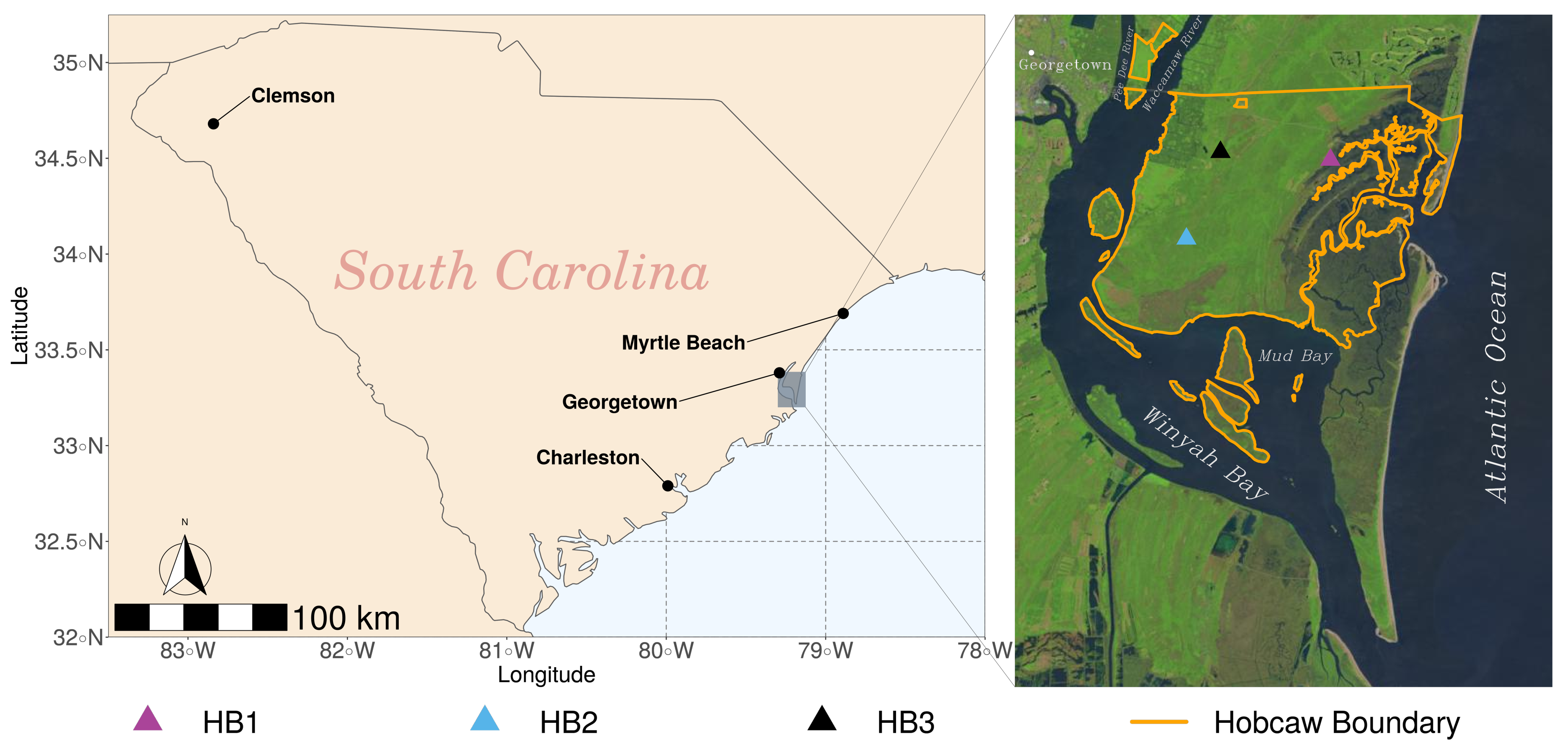
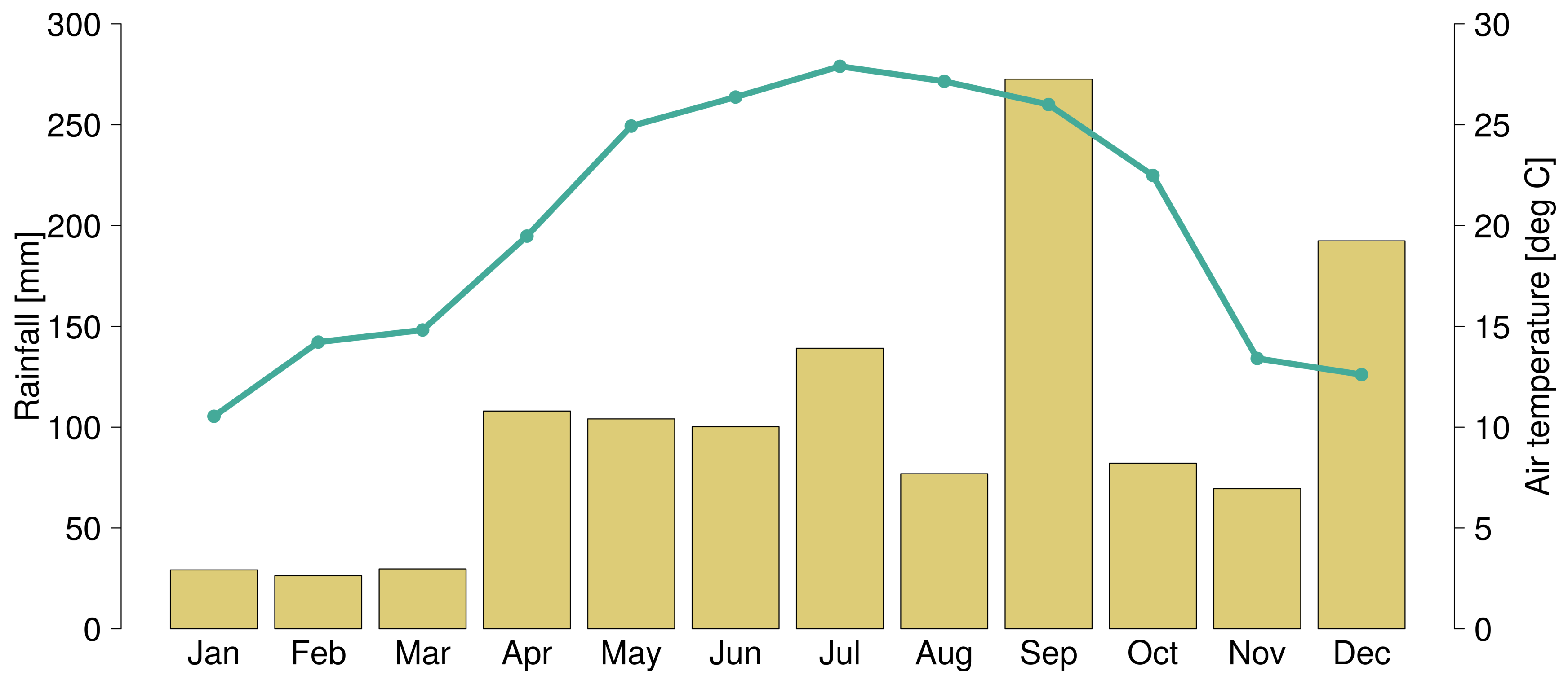
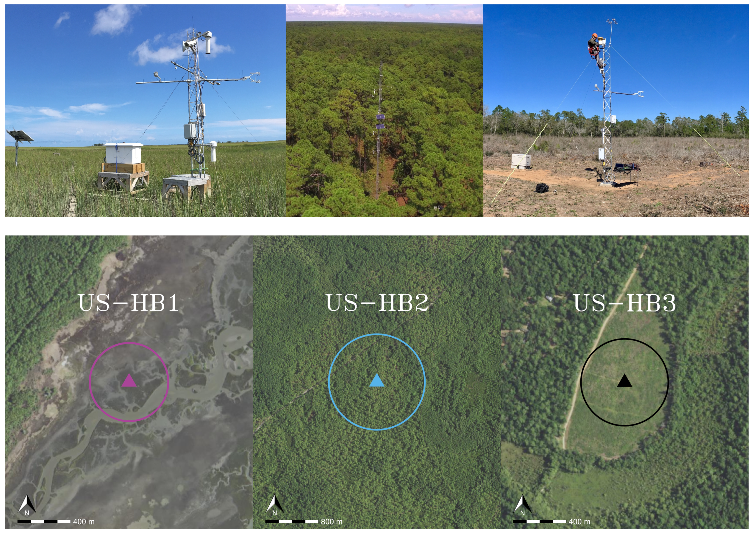
3.1. Site Description

The data described in this manuscript originate from eddy covariance flux towers located on Hobcaw Barony, an approximately 6400 ha parcel of private land that comprises the southern end of the Waccamaw Neck peninsula just outside of Georgetown, South Carolina. The property is owned and managed by the Belle W. Baruch Foundation with the mission to “conserve Hobcaw Barony’s unique natural and cultural resources for research and education” (http://hobcawbarony.org/about-hobcaw/). The property connects to the rest of the Waccamaw Neck to the north and is bounded by the Waccamaw River to the west, the Winyah Bay estuary to the south, and the Atlantic Ocean to the east, as illustrated in Figure 2. Approximately half of the property is forested, where higher elevations are dominated by southern pine species with loblolly (Pinus taeda) and longleaf (Pinus palustris) pine in the majority, and lower elevations contain seasonally and permanently flooded swamps containing baldcypress (Taxodium distichum (L.) Rich.), water tupelo (Nyssa aquatica L.) and swamp blackgum (Nyssa biflora Walt.). The eastern half of the property is the North Inlet salt marsh, which experiences semidiurnal tides with a 1.4m mean range and is dominated by a near monoculture of smooth cordgrass (Spartina alterniflora). The North Inlet marsh is contained in the North Inlet-Winyah Bay National Estuarine Research Reserve (NI-WB NERR) and has been the subject of extensive study (e.g., Morris et al. [35]). The property is home to Clemson University’s Baruch Institute of Coastal Ecology and Forest Science and the University of South Carolina’s Belle W. Baruch Institute for Marine and Coastal Sciences. The climate at the site is hot with humid summers and mild winters (Figure 3) and is classified as Cfa (humid subtropical climates) in the Köppen–Geiger climate classification system [36].

Figure 2. Map of South Carolina showing the mesonet’s study region in reference to major cities. The inset is a satellite image marked with each tower’s coordinates, the boundary of the land grant (Hobcaw Barony), nearest town (Georgetown, SC), and local waterways (Landsat-7 image courtesy of the U.S. Geological Survey).

Figure 3. Precipitation and air temperature variables at the Hobcaw Barony sites for the period of January 2019 through December 2019. The bars are total precipitation for each month measured for US-HB1 (via the North Inlet-Winyah Bay National Estuarine Research Reserve (NI-WB NERR)). The line illustrates the mean monthly air temperature measured at US-HB2 (TA_1_1_1). Note the high precipitation values for September, when Hurricane Dorian made landfall in South Carolina.

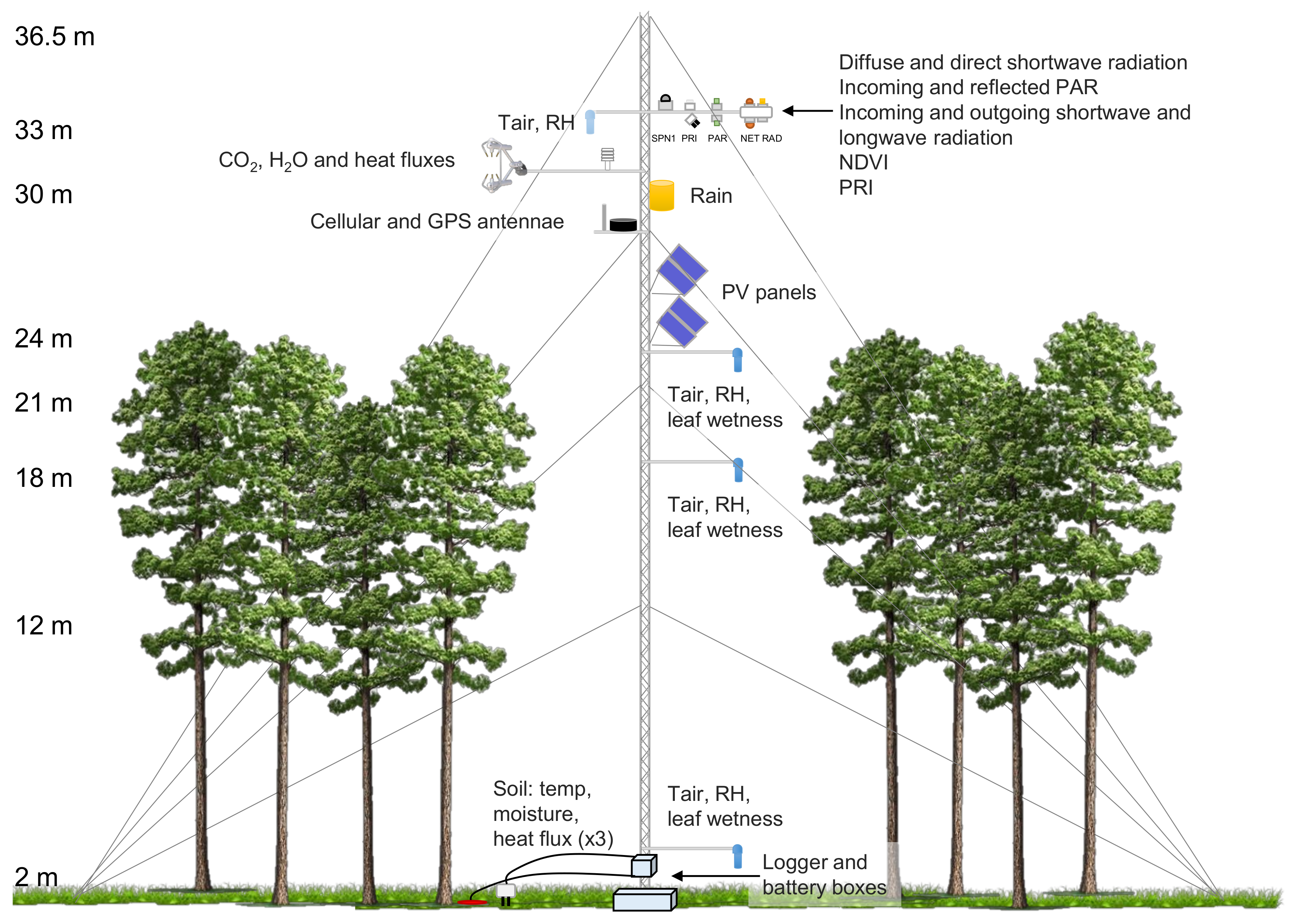
Tower Locations and Infrastructure

US-HB1 is a 5 m tall triangular aluminum tower located in a tidally-influenced Spartina alterniflora salt marsh (Figure 4) accessed by and located along a wooden boardwalk used as part of long term System-Wide Monitoring Program (SWMP) sampling within the North Inlet-Winyah Bay National Estuarine Research Reserve (NI-WB NERR). It is approximately 200 m from the forest edge and 60 m from Crab Haul Creek, which is monitored for water quality approximately 950 m downstream of the tower (creek distance) at the Oyster Landing NOAA tide gauge (Station ID: 8662245). Eddy covariance instrumentation was placed at a height that limited the majority (90%) of the flux footprint within the Spartina zone of the marsh platform. This was determined using initial turbulence data and a footprint model [37]. The result is that the 90th percentile of the flux footprint has a radius of 90 m and comprises approximately 40% tall form Spartina, 40% short form Spartina, and 20% creek. Radiometers were placed as high as logistically possible and have a clear optical footprint of Spartina grass canopy. The tower base elevation is approximately 0.10 m (NAVD88) and the mean tidal range is 1.4 m such that the marsh platform and creek beds can be without water at low tide and the marsh platform under the tower inundated by about 0.60 m of water on a typical high tide. The long term salinity at Oyster Landing is 32 PSU. Soils at US-HB1 are classified as Bohicket silty clay loam, which is characterized by frequent flooding and being very poorly drained with a 0% to 1% slope, an average pH of 7.3, 0.04 $\frac{cm}{cm}$ available water capacity, 13.09% soil organic matter (SOM), and 1.41 $\frac{g}{c{m}^3}$ bulk density (at −0.03 MPa), according to the USDA Natural Resources Conservation Service (NRCS) Web Soil Survey (WSS) [38]. Electrical power is supplied to the instruments by a 100 Watt photovoltaic system with the solar panels installed on a separate post. The tower became operational in May of 2017, was largely destroyed by Hurricane Dorian in September of 2019, but was rebuilt and operational again by December of that same year.

Figure 4. Top row left to right: US-HB1, US-HB2, US-HB3 tower locations. Bottom row left to right: approximate 90th percentile of the flux footprint for each tower overlayed on top of aerial photographs accessed through the Aerial Photography Field Office (APFO) National Agriculture Imagery Program’s (NAIP) Public Server (https://gis.apfo.usda.gov/arcgis/rest/services). Target footprints have a radius of 90, 220 and 100 m for US-HB1, US-HB2, and US-HB3, respectively.

US-HB2 is a 36.5 m tall triangular galvanized steel tower located in a mature southern pine forest on Hobcaw Barony. The tower base elevation is 4.2 m (NAVD88) and the tower is approximately 3.0 km west of the salt marsh and 7.8 km west of the Atlantic Ocean. Eddy covariance instrumentation was placed at a height that limited the majority (90%) of the flux footprint within a single forest management unit that is bounded by dirt roads to the east and west of the tower. The 90th percentile of the flux footprint has a radius of 200 m and the tree species distribution in the footprint is approximately 42%, 24% and 18%, longleaf (Pinus palustris), loblolly (Pinus taeda), and pond (Pinus serotina) pine, respectively. The remaining 16% are hardwoods primarily consisting of water tupelo (Nyssa aquatica), water oak (Quercus nigra), and swamp tupelo (Nyssa biflora) found in a hardwood drain near the eastern edge of the footprint. Tree density is 340 $\frac{stems}{ha}$ with a basal area of 240 $\frac{m^2}{ha}$ and average tree height of approximately 14 m (maximum height 23 m) for all stems ≥10 cm. The understory is dominated by woody growth from plants such as inkberry (Ilex glabra), redbay (Persea borbonia), highbush blueberry (Vaccinium corymbosum), sweetgum (Liquidambar styraciflua), and fetterbush (Lyonia lucida). Soils at US-HB2 are classified as poorly drained Leon sand with a 0% to 2% slope, which is characterized by an average pH of 4.7, 0.05 $\frac{cm}{cm}$ available water capacity, 1.51% soil organic matter (SOM), and 1.56 $\frac{g}{c{m}^3}$ bulk density (at −0.03 MPa), according to the USDA NRCS Web Soil Survey (WSS) [38]. The site is actively managed with fire to subdue these understory species and promote pine regeneration. Here the electrical power is supplied to the instruments by a 275 Watt photovoltaic system, with the solar panels mounted on the tower just above the tree canopy. Radiometers were placed as high as logistically possible. This tower became operational in April of 2018.

US-HB3 is a 6.1 m tall triangular aluminum tower located in a 6.7 ha young longleaf pine plantation. The prior land use was a mature, mixed hardwood-pine forest. That stand was harvested by clearcut in 2016 and prepared with herbicide in the summer of 2017. In March, 2018 the stand was handplanted by hoedad with containerized longleaf pine seedlings (open pollinated) on a 8′ × 10′ (2.44 m × 3.04 m) spacing totaling 544 seedlings per acre (≈1344 per ha). In 2019 some dead seedlings were replaced by spot planting. Soils at US-HB3 are classified as excessively drained Lakeland fine sand with a 0% to 6% slope, which is characterized by an average pH of 5.3, 0.06 $\frac{cm}{cm}$ available water capacity, 0.55% soil organic matter (SOM), and 1.52 $\frac{g}{c{m}^3}$ bulk density (at −0.03 MPa), according to the USDA NRCS Web Soil Survey (WSS) [38]. The eddy covariance tower was constructed in the approximate widest point of the lachrymiform field, where the continuous clearcut fetch is 100 m in the shortest dimension and up to 260 m in the longest dimension. Sensor heights were optimized using initial turbulence data and a flux footprint model [37] to limit 95% of the flux footprint within a 100 m radius. The effect of the vertical growth of trees on the flux footprint will be reexamined each year and sensor height will be adjusted if needed. Radiometers were placed as high as logistically possible. Electrical power is supplied to the instruments by a 100 Watt photovoltaic system with the solar panels installed on a separate post. The tower became operational in January of 2019.

3.2. Sensors

Each site was constructed as a replicate suite of sensors designed to measure the carbon, water, and energy fluxes between the land and the atmosphere, as well as meteorological, phenological and soil variables. Essentially each site is identical with differences in the height of the towers and the number of sensors as the result of placement in differing habitat types. Table A1 in the appendix summarizes the sensors deployed at each tower, the measured and primary derived variables produced by each sensor, the height on the tower, and number of replicates of each sensor. As previously mentioned, much of this information is also captured in the BADM metadata.

Common sensors installed at all three sites include the IRGASON C2${}_2$/H2O Open Path Gas Analyzer System W/Sonic (Campbell Scientific Inc., Logan, UT, USA), CNR4 Net Radiometer (Kipp and Zonen, Delft, The Netherlands), SRS Spectral Reflectance Sensors (Meter Group Inc., Pullman, Washington, USA), and the HMP155 Humidity and Temperature Probe (Vaisala, Helsinki, Finland). The IRGASONs produce measurements of carbon dioxide and water vapor concentrations, air temperature, and 3-D wind velocity at 10 Hz. The CNR4 Net Radiometers measure incoming and outwelling shortwave and longwave radiation and the SRS measure incoming and reflected narrow band radiation. The HMP155 measures air temperature (${}^{\circ }$C) and relative humidity (%). See Figure 5 for a diagram of approximate sensor arrangement on US-HB2.

Figure 5. Schematic of eddy covariance tower US-HB2, indicating the location of instrumentation.

Additional measures of meteorological radiation are provided by the SQ-500 Full Spectrum Quantum Sensor (Apogee Instruments, Inc., Logan, UT, USA) at US-HB2 and US-HB3, and the SPN1 Sunshine Pyranometer (Delta-T Devices LTD, Cambridge, UK) at US-HB2. The SQ-500 measures photosynthetic photon flux density while the SPN1 measures total (direct plus diffuse) and diffuse incident solar radiation. Barometric pressure is measured with the PTB110 Barometric Pressure Sensor (Vaisala, Helsinki, Finland) only at one tower, US-HB3 at a height of 1.5 m. Rainfall is measured by the TE525 Tipping Bucket Rain Gage (Texas Electronics, Dallas, TX, USA). Soil variables measured include soil temperature and volumetric soil moisture content. At US-HB2 and US-HB3, the CS655 Water Content Reflectometer (Campbell Scientific Inc., Logan, UT, USA) measures these variables. Only soil temperature is measured at US-HB1 with 109SS Temperature Probes (Campbell Scientific Inc., Logan, UT, USA) because the soil is continuously saturated. Soil heat flux is measured with HFP01 Heat Flux Plates (Hukseflux Thermal Sensors B.V., Delft, The Netherlands) at both US-HB2 and US-HB3, which have 3 replicates. A physical measure of leaf wetness is estimated by inference with a LWS Dielectric Leaf Wetness Sensor (Meter Group Inc., Pullman, Washington, USA) at two sites, US-HB2 and US-HB3 with replicates at multiple heights.

3.3. Raw Measurements

Raw flux variables were recorded at 10 Hz (carbon dioxide and water vapor concentration, sonic temperature, and 3-D wind velocity) and most meteorological measurements were made every 15 s and averaged or summed in the logger memory to record 1-min values on a CR6 Measurement and Control DataLogger (Campbell Scientific Inc., Logan, UT, USA) at US-HB2 and US-HB3. At US-HB1, prior to Hurricane Dorian, 10 Hz (flux) variables were recorded on a CR6 while 1-minute variables were recorded on a CR800 Measurement and Control DataLogger (Campbell Scientific Inc., Logan, UT, USA). Since rebuilding US-HB1 after Hurricane Dorian, all variables were recorded on a CR6 Measurement and Control DataLogger.

Gas concentrations of CO${}_2$ ($\frac{mg}{m^3}$), water vapor ($\frac{g}{m^3}$) and sonic air temperature (${}^{\circ }$C) were measured by the IRGASON Integrated CO${}_2$/H${}_2$O Open-Path Gas Analyzer and 3D Sonic Anemometer. Wind speed ($\frac{m}{s}$) was measured in three directions: vertical, meridional, and zonal. The IRGASON EC100 system also measured air temperature (${}^{\circ }$C) and barometric pressure (kPa). An independent measure of barometric pressure (kPa) from the IRGASONs was measured with the PTB110 Barometric Pressure Sensor only at US-HB3.

Each of the three sites also measured meteorological variables including atmospheric humidity and temperature, incoming and reflected radiation, and soil water content and temperature. Air temperature (${}^{\circ }$C) and relative humidity (%) were measured with the HMP155 Humidity and Temperature Probe. Rainfall (mm) was measured with the TE525 Tipping Bucket Rain Gauge at US-HB2 and US-HB3. The TE525 measured rainfall (mm) as 0.1 mm of rainfall per tip. There was no measured rainfall at US-HB1 due to its proximity (within 800 m) to the NI-WB NERR weather station at Oyster Landing, which provides publicly accessible weather data, including precipitation [39], and uses a similar tipping bucket rain gauge. Incoming and reflected short-wave solar radiation ($\frac{W}{m^2}$) and incoming and emitted long-wave far infrared radiation ($\frac{W}{m^2}$) were measured with the CNR4 Net Radiometer. Another measure of incoming short-wave radiation was measured at US-HB2 with the SPN1 Sunshine Pyranometer. The SPN-1 measured total and diffuse short-wave radiation. Incoming and reflected PAR, photosynthetically active radiation, ($\frac{\mu molPhoton}{m^2·s}$) were measured at US-HB2 and US-HB3 with the SQ-500 Full Spectrum Quantum Sensors. Spectral Reflectance Sensors (SRS) measured incident and reflected radiation in narrow wavebands necessary for calculating the NDVI—Normalized Difference Vegetation Index, and PRI—Photochemical Reflectance Index. Hemispherical SRS sensors, PRI (Pi) and NDVI (Ni), measured incident radiation $\frac{W}{m^2·nm}$. Field Stop SRS sensors, PRI (Pr) and NDVI (Nr), measured reflected radiation $\frac{W}{m^2·nmsr}$. US-HB2 and US-HB3 had all four SRS sensors. US-HB1 only had SRS sensors for NDVI calculations.

Soil volumetric water content (%), bulk electrical conductivity ($\frac{dS}{m}$) and temperature (${}^{\circ }$C) were measured with the CS655 Water Content Reflectometers at US-HB2 and US-HB3. US-HB1 only had a measure of soil temperature (${}^{\circ }$C) measured with the 109SS Temperature Probe. Soil heat flux ($\frac{W}{m^2}$) was measured with the HFP01 Heat Flux Plates. Soil heat flux was measured at two tower sites, US-HB2 and US-HB3. The wetness of nearby leaves at US-HB2 and US-HB3 was estimated by inference with a LWS Dielectric Leaf Wetness Sensor. The LWS measured the dielectric constant of the sensor’s upper surface (mv) which was converted to leaf wetness (%) later in data processing.

3.4. Data Storage

Raw data were stored at the sites on 16 GB microSD flash SLC memory cards which are part of the CR6 Measurement and Control DataLogger. Every 2 weeks, the raw Time Series and Meteorological data files (.DAT) were transferred to a laptop for transport back to the office for processing. To save space, at the time of data transfer, the memory card was cleaned of older files which had already been post processed by that time. At the lab, the laptop was connected to the server and the raw data files were copied to a long term data storage computer. In addition, raw data files were copied to a data processing computer for use, sharing within the lab, and further processing. This computer was synced to a cloud drive to allow remote access for other users and to create a third repository for the data. The CardConvert utility of the LoggerNet software (Campbell Scientific Inc., Logan, UT, USA) was used to convert the TOB3 (Campbell Scientific proprietary file type; .DAT) binary raw data files to array compatible comma-separated values (.CSV) files, a simple delimited text file format accessible by a wide range of computer software. The meteorological data CSVs contained approximately 2 weeks of data and were in a 1-minute data format with timestamps converted to columns for year, Julian date, and time (24 h, hhmm). Time series CSVs contained 30 minutes of data and were in a 10 hz data format with timestamps converted to columns for year, Julian date, time (24 hr, hhmm), and tenths of a second.

3.5. Data Quality Assurance/Quality Control (QA/QC)

Both meteorological and time series CSVs were subjected to our own Quality Assurance/Quality Control (QA/QC) check by using an R Markdown script with R and Python code prior to post processing. The script generated pdf files with summary tables and graphs of all of the meteorological and high frequency time series variables for the two week period, as well as a table with the number of points and percentage of time outside of preset tolerances. The time series QA/QC PDFs also contained tables of flags, descriptors, and codes of the IRGASON sonic anemometer and open-path gas analyzer diagnostic values. The primary goal of this QA/QC process was to catch anomalies quickly and make repairs or adjustments to sensors in the field as needed.

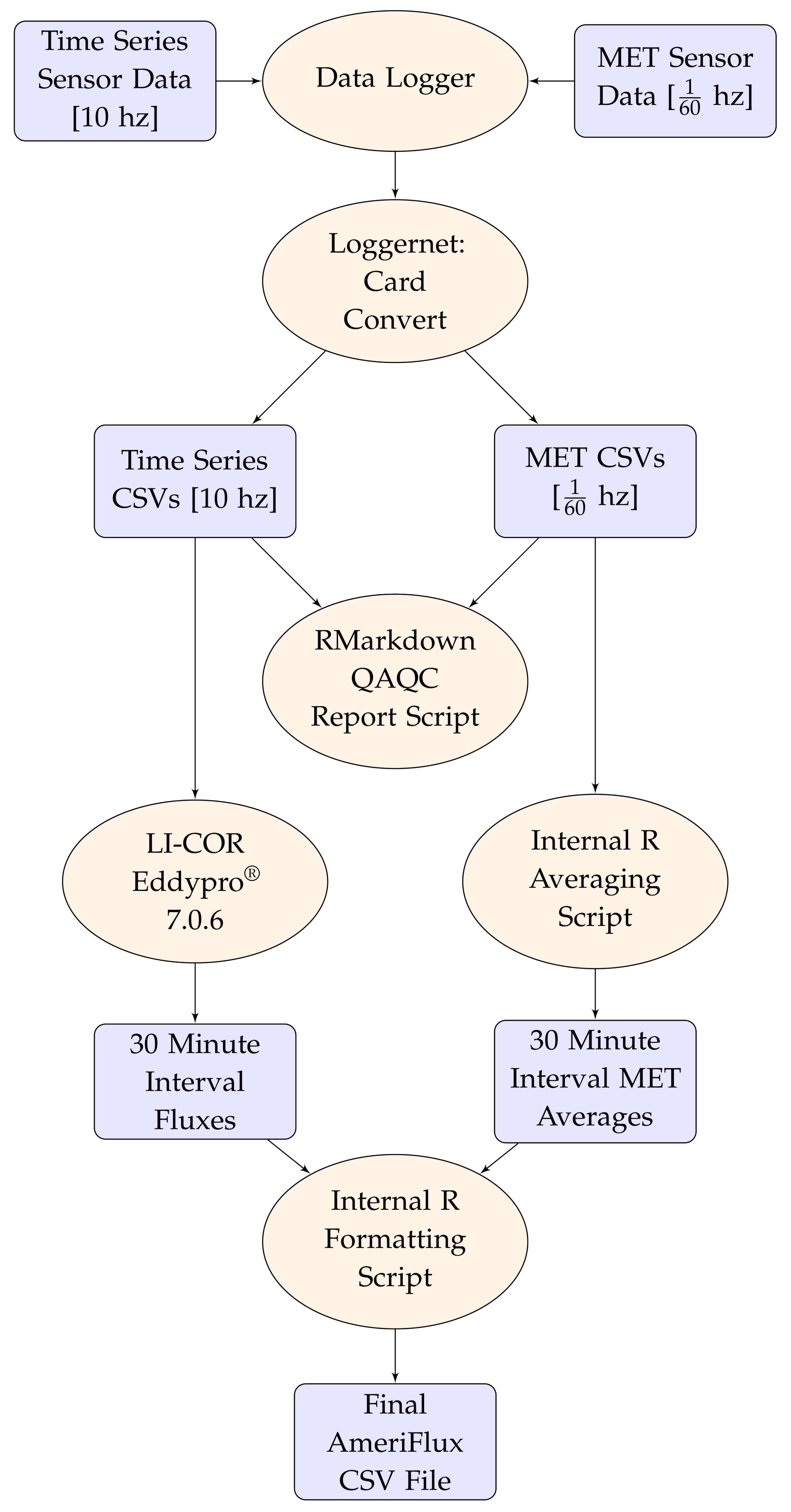
3.6. Data Processing and Derived Variables

The raw high frequency (10 hz) eddy covariance data contained within the time series CSVs were processed with EddyPro^® v7.0.6 (LI-COR Biosciences, Lincoln, NE, USA) to calculate the 30 min interval turbulent fluxes, including carbon dioxide (FC), momentum (TAU), latent heat (LE), and sensible heat (H). We used the micrometeorological sign convention, defining flux emitted from the ecosystem to the atmosphere as a positive value, while flux into the ecosystem (i.e., carbon dioxide used by the biosphere) is a negative value. Additional derived variables included storage fluxes (SC, SLE, SH), statistical footprint estimations (FETCH), vapor pressure deficit (VPD), Monin–Obukhov length and stability (MO_LENGTH, ZL), and friction velocity (USTAR). Quality flags (0,1,2) were calculated from the steady state and integral turbulence characteristics (SS_ITC_TEST) as per the Foken et al. 2004 protocol [34]. It is our recommendation that fluxes that score a “2” in this system are discarded before analysis. In addition, note: the flux data were not gap filled, per AmeriFlux protocols. To generate the EddyPro^® output file we used the “thorough” output setting which writes an assortment of files, including a FLUXNET formatted CSV, which forms the basis of the archived AmeriFlux dataset. For an overview of the custom settings we select within the EddyPro^® software see Appendix A Table A2.

An additional step was required to produce the AmeriFlux variables C2${}_2$_SIGMA and H${}_2$O_SIGMA, which report the standard deviations of the CO${}_2$ mole fraction and H${}_2$O mole fraction as mixing ratios ($\frac{mmol}{mol}$), due to the units that IRGASON records these values in (mass density, $\frac{mmol}{m^3}$). To achieve the desired output we used the Eddypro^® level 6 statistical calculation files to manually calculate the standard deviations after converting the values at each timestep to mixing ratios. This procedure took place within the internal R formatting script detailed below.

The FLUXNET-formatted EddyPro^® output CSV was combined with averages from the meteorological variables for the same 30 min intervals with an R script. Before those averages were calculated, the meteorological variables were filtered based on a set of site-specific tolerances. The original data files were not overwritten and this step occurred only in the data processing computer’s memory within the R script. The time series data were not filtered prior to processing, but the raw 10 hz measurements were first filtered in EddyPro^® using default settings under the Statistical Analysis menu. The derived variables are later checked against a range of plausible values after processing but before submission to AmeriFlux. Data ranges that defined these filters are listed in the Appendix A Table A3. The R script also formats those data to match the AmeriFlux requirements, including converting units on several variables and appending AmeriFlux column headers. A value of −9999 was inserted into any gaps in the data before the final composite file was submitted to the AmeriFlux website.

4. Conclusions

This new coastal flux mesonet and accompanying datasets should be useful for studying carbon, water and energy cycling in understudied coastal ecosystems of the Southeastern U.S., including salt marshes and longleaf pine forests. Co-location of the three sites ensures they receive the same meteorological conditions, so differences in fluxes between sites result almost entirely from their differing physiologies, with one major exception: US-HB1 experiences regular tidal inundation. The proximity of a tidal wetland eddy flux site (which are relatively rare) to upland sites (US-HB3 is 3.4 km west of US-HB1) may be one of the most unique elements of this dataset. The effect of flooding on the energy balance at US-HB1 is apparent even in the mean annual diurnal cycle (Figure 6). The salt marsh generates more latent heat flux through evapotranspiration and exhibits less-pronounced diurnal cycling compared to terrestrial systems because the biological processes are linked to tidal flooding in addition to solar cycles. The pair of newly-restored longleaf pine plantation (post clearcut) with a mature longleaf pine site is also unique. Differences in fluxes there (Figure 7) result (presumably) from the large difference in biomass, canopy height, roughness and leaf area. We anticipate this dataset will expand and be updated in coming years. Since these sites are located on the same property as the host institute and are partially maintained with institutional technician support, our goal is to operate these sites for at least several years. The mesonet itself will also continue to expand, as a fourth tower, in an impounded, managed, brackish wetland, has recently come online (April 2020). The latest mesonet information is available at https://sites.google.com/g.clemson.edu/ohalloran/.

Figure 6. The diurnal patterns of fluxes of carbon dioxide, sensible heat, and latent heat averaged over the entire year of 2019. The mature southern pine forest (US-HB2) exhibits the strongest daytime carbon uptake of the three sites. The salt marsh (US-HB1) has the highest latent heat flux (evapotranspiration) due to saturated soils, which, combined with lateral tidal heat exchange, reduces the sensible heat flux.

Figure 7. The carbon dioxide, sensible heat, and latent heat turbulent fluxes for all three tower locations spanning the year 2019. While US-HB1 and US-HB3 (salt marsh and recent pine clearcut harvest, respectively) show some seasonality with larger fluxes of carbon dioxide and heat in the summer months, US-HB2 (mature pine forest) does not. This lack of seasonality is particularly evident with carbon dioxide, where the mature pine ecosystem’s photosynthesis does not drastically decline in the winter as a deciduous forest ecosystem would be expected to. Note: US-HB1 has a data gap from September 1st 15:00 EST through December 5th 10:00 EST due to damage from Hurricane Dorian.

References

- Friedlingstein, P.; Jones, M.W.; O’Sullivan, M.; Andrew, R.M.; Hauck, J.; Peters, G.P.; Peters, W.; Pongratz, J.; Sitch, S.; Le Quéré, C.; et al. Global carbon budget 2019. Earth Syst. Sci. Data 2019, 11, 1783–1838. [Google Scholar] [CrossRef]
- Bruhwiler, L.; Birdsey, A.M.M.R.; Fisher, J.B.; Houghton, R.A.; Huntzinger, D.N.; Miller, J.B. Synthesis. In Second State of the Carbon Cycle Report (SOCCR2); U.S. Global Change Research Program (USGCRP): Washington, DC, USA, 2018; Chapter 1–2; pp. 42–108. [Google Scholar] [CrossRef]
- Terziyski, A.; Tenev, S.; Jeliazkov, V.; Jeliazkova, N.; Kochev, N. METER.AC: Live open access atmospheric monitoring data for bulgaria with high spatiotemporal resolution. Data 2020, 5, 36. [Google Scholar] [CrossRef]
- Daley, R. Preface to Atmospheric Data Analysis. In Atmospheric Data Analysis, Reprint ed.; Cambridge University Press: New York, NY, USA, 1996; Chapter 1. [Google Scholar]
- Baldocchi, D.D. Assessing the eddy covariance technique for evaluating carbon dioxide exchange rates of ecosystems: Past, present and future. Glob. Chang. Biol. 2003, 9, 479–492. [Google Scholar] [CrossRef]
- Overpeck, J.; Meehl, G.; Bony, S.; Easterling, D. Climate Data Challenges in the 21st Century. Science 2011, 331, 700–702. [Google Scholar] [CrossRef]
- Windham-Myers, L.; Cai, W.J.; Alin, S.; Andersson, A.; Crosswell, J.; Dunton, K.H.; Hernandez-Ayon, J.M.; Herrmann, M.; Hinson, A.L.; Hopkinson, C.S.; et al. Tidal Wetlands and Estuaries. In Second State of the Carbon Cycle Report (SOCCR2); U.S. Global Change Research Program (USGCRP): Washington, DC, USA, 2018; Chapter 15; pp. 596–648. [Google Scholar] [CrossRef]
- Twigg, E. Coastal Blue Carbon Approaches for Carbon Dioxide Removal and Reliable Sequestration: Proceedings of a Workshop in Brief. In National Academies of Sciences, Engineering, and Medicine 2017; The National Academies Press: Washington, DC, USA, 2017. [Google Scholar] [CrossRef]
- Holmquist, J.R.; Windham-Myers, L.; Bernal, B.; Byrd, K.B.; Crooks, S.; Gonneea, M.E.; Herold, N.; Knox, S.H.; Kroeger, K.D.; McCombs, J.; et al. Uncertainty in United States coastal wetland greenhouse gas inventorying. Environ. Res. Lett. 2018, 13. [Google Scholar] [CrossRef]
- Barbier, E.B.; Hacker, S.D.; Kennedy, C.; Koch, E.W.; Stier, A.C.; Silliman, B.R. The value of estuarine and coastal ecosystem services. Ecol. Monogr. 2011, 81, 169–193. [Google Scholar] [CrossRef]
- Temmerman, S.; Meire, P.; Bouma, T.J.; Herman, P.M.; Ysebaert, T.; De Vriend, H.J. Ecosystem-based coastal defence in the face of global change. Nature 2013, 504, 79–83. [Google Scholar] [CrossRef]
- Lu, X.; Kicklighter, D.W.; Melillo, J.M.; Reilly, J.M.; Xu, L. Land carbon sequestration within the conterminous United States: Regional- and state-level analyses. J. Geophys. Res. Biogeosci. 2015, 120, 379–398. [Google Scholar] [CrossRef]
- Johnsen, K.H.; Wear, D.; Oren, R.; Teskey, R.O.; Sanchez, F.; Will, R.; Butnor, J.; Markewitz, D.; Richter, D.; Rials, T.; et al. Carbon Sequestration and Southern Pine Forests Land Use: A Major Determinant. J. For. 2001, 99, 14–21. [Google Scholar]
- Oswalt, S.N.; Smith, W.B.; Miles, P.D.; Pugh, S.A. Forest Resources of the United States, 2017; Technical Report WO-97; USDA Forest Service: Washington, DC, USA, 2019. [CrossRef]
- Sedjo, R.; Sohngen, B. Carbon Sequestration in Forests and Soils. Annu. Rev. Resour. Econ. 2012, 4, 127–144. [Google Scholar] [CrossRef]
- Huntzinger, D.N.; Michalak, A.M.; Schwalm, C.; Ciais, P.; King, A.W.; Fang, Y.; Schaefer, K.; Wei, Y.; Cook, R.B.; Fisher, J.B.; et al. Uncertainty in the response of terrestrial carbon sink to environmental drivers undermines carbon-climate feedback predictions. Sci. Rep. 2017, 7, 1–8. [Google Scholar] [CrossRef] [PubMed]
- Frost, C.C. Four centuries of changing landscape patterns in the longleaf pine ecosystem. In Proceedings of the Tall Timbers Fire Ecology Conference No. 18, The Longleaf Pine Ecosystem: Ecology, Restoration and Management; Tallahassee, FL, USA, 30 May–2 June 1993, Hermann, S.M., Ed.; Tall Timbers Research Station: Tallahassee, FL, USA, 1993; Volume 18, pp. 17–43. [Google Scholar]
- Jose, S.; Jokela, E.J.; Miller, D.L. The Longleaf Pine Ecosystem. In The Longleaf Pine Ecosystem: Ecology, Silviculture, and Resoration, 1st ed.; Springer: New York, NY, USA, 2007; Chapter 1; pp. 3–8. [Google Scholar]
- Van Lear, D.H.; Carroll, W.D.; Kapeluck, P.R.; Johnson, R. History and restoration of the longleaf pine-grassland ecosystem: Implications for species at risk. For. Ecol. Manag. 2005, 211, 150–165. [Google Scholar] [CrossRef]
- Darden, T.; Case, D.; Hayes, L.; Gjerstad, D.; Sutter, R.; Bohn, C.; Demarest, D. Range-Wide Conservation Plan for Longleaf Pine; Technical report, America’s Longleaf - A Restoration Initiative for the Southern Longleaf Pine Forest. 2009. Available online: http://americaslongleaf.org/media/fqipycuc/conservation$_$plan.pdf (accessed on 3 September 2020).
- Mcintyre, R.K.; Guldin, J.M.; Ettel, T.; Ware, C.; Jones, K. Restoration of longleaf pine in the southern United States: A status report. In Proceedings of the 19th biennial southern silvicultural research conference, Blacksburg, VA, USA, 14–16 March 2017; e-Gen. Tech. Rep. SRS-234. U.S. Department of Agriculture Forest Service, Southern Research Station: Asheville, NC, USA, 2018; pp. 297–302. [Google Scholar]
- Brantley, S.T.; Vose, J.M.; Wear, D.N.; Band, L. Planning for an uncertain future: Restoration to mitigate water scarcity and sustain carbon sequestration. In Ecological Restoration and Management of Longleaf Pine Forests; CRC Press: Boca Raton, FL, USA, 2017; Chapter 15; pp. 291–310. [Google Scholar]
- Sun, G.; Noormets, A.; Gavazzi, M.J.; McNulty, S.G.; Chen, J.; Domec, J.C.; King, J.S.; Amatya, D.M.; Skaggs, R.W. Energy and water balance of two contrasting loblolly pine plantations on the lower coastal plain of North Carolina, USA. For. Ecol. Manag. 2010, 259, 1299–1310. [Google Scholar] [CrossRef]
- Noormets, A.; Gavazzi, M.J.; McNulty, S.G.; Domec, J.C.; Sun, G.; King, J.S.; Chen, J. Response of carbon fluxes to drought in a coastal plain loblolly pine forest. Glob. Chang. Biol. 2010, 16, 272–287. [Google Scholar] [CrossRef]
- Clark, K.L.; Gholz, H.L.; Castro, M.S. Carbon dynamics along a chronosequence of slash pine plantations in North Florida. Ecol. Appl. 2004, 14, 1154–1171. [Google Scholar] [CrossRef]
- Powell, T.L.; Gholz, H.L.; Clark, K.L.; Starr, G.; Cropper, W.P.; Martin, T.A. Carbon exchange of a mature, naturally regenerated pine forest in north Florida. Glob. Chang. Biol. 2008, 14, 2523–2538. [Google Scholar] [CrossRef]
- Kathilankal, J.C.; Mozdzer, T.J.; Fuentes, J.D.; D’Odorico, P.; McGlathery, K.J.; Zieman, J.C. Tidal influences on carbon assimilation by a salt marsh. Environ. Res. Lett. 2008, 3. [Google Scholar] [CrossRef]
- Krauss, K.W.; Holm, G.O.; Perez, B.C.; McWhorter, D.E.; Cormier, N.; Moss, R.F.; Johnson, D.J.; Neubauer, S.C.; Raynie, R.C. Component greenhouse gas fluxes and radiative balance from two deltaic marshes in Louisiana: Pairing chamber techniques and eddy covariance. J. Geophys. Res. Biogeosci. 2016, 121, 1503–1521. [Google Scholar] [CrossRef]
- Barr, J.G.; Engel, V.; Fuentes, J.D.; Zieman, J.C.; O’Halloran, T.L.; Smith, T.J.; Anderson, G.H. Controls on mangrove forest-atmosphere carbon dioxide exchanges in western Everglades National Park. J. Geophys. Res. Biogeosci. 2010, 115. [Google Scholar] [CrossRef]
- Campioli, M.; Malhi, Y.; Vicca, S.; Luyssaert, S.; Papale, D.; Peñuelas, J.; Reichstein, M.; Migliavacca, M.; Arain, M.A.; Janssens, I.A. Evaluating the convergence between eddy-covariance and biometric methods for assessing carbon budgets of forests. Nat. Commun. 2016, 7, 1–12. [Google Scholar] [CrossRef]
- Baldocchi, D. Measuring fluxes of trace gases and energy between ecosystems and the atmosphere - the state and future of the eddy covariance method. Glob. Chang. Biol. 2014, 20, 3600–3609. [Google Scholar] [CrossRef] [PubMed]
- Burba, G.; Anderson, D. A Brief Practical Guide to Eddy Covariance Flux Measurements: Principles and Workflow Examples for Scientific and Industrial Applications, 1.0.1 ed.; LI-COR Biosciences: Lincoln, NE, USA, 2010; p. 212. [Google Scholar]
- Law, B.E. AmeriFlux Network Aids Global Synthesis. Eos 2007, 88. [Google Scholar] [CrossRef]
- Foken, T.; Mathias, G.; Mauder, M.; Mahrt, L.; Amiro, B.; Munger, W. Post-field data quality control. In Handbook of Micrometeorology; Springer: Dordrecht, The Netherlands, 2004; Chapter 9. [Google Scholar] [CrossRef]
- Morris, J.T.; Sundberg, K.; Hopkinson, C.S. Salt marsh primary production and its responses to relative sea level and nutrientsin estuaries at plum island, Massachusetts, and North Inlet, South Carolina, USA. Oceanography 2013, 26, 78–84. [Google Scholar] [CrossRef]
- Kottek, M.; Grieser, J.; Beck, C.; Rudolf, B.; Rubel, F. World map of the Köppen-Geiger climate classification updated. Meteorol. Z. 2006, 15, 259–263. [Google Scholar] [CrossRef]
- Kljun, N.; Calanca, P.; Rotach, M.W.; Schmid, H.P. A simple parameterisation for flux footprint predictions. Bound.-Layer Meteorol. 2004, 112, 503–523. [Google Scholar] [CrossRef]
- Staff. Web Soil Survey. Natural Resources Conservation Service, United States Department of Agriculture. Available online: https://websoilsurvey.sc.egov.usda.gov/ (accessed on 1 August 2012).
- NOAA NERRS Centralized Data Management Office. System-Wide Monitoring Program. Data Accessed from the NOAA NERRS Centralized Data Management Office. Available online: http://www.nerrsdata.org (accessed on 15 July 2020).
Publisher’s Note: MDPI stays neutral with regard to jurisdictional claims in published maps and institutional affiliations. |
© 2020 by the authors. Licensee MDPI, Basel, Switzerland. This article is an open access article distributed under the terms and conditions of the Creative Commons Attribution (CC BY) license (http://creativecommons.org/licenses/by/4.0/).