1. Introduction
The history of earth observation data, and evolution of information technology and the internet have created a transition of scene-based and project-based thinking to imagery as a seamless time series. Killough (2018) described a goal of the CEOS Open Data Cube as increased global impact of satellite data. To achieve this goal, we see four requirements, some already in process, all still evolving.
The first three decades of Landsat and the broader earth observation community were dominated by specialists working on individual projects often on individual satellite scenes of a single date or a few dates from a single senor. The data was expensive, required special software and knowledge to extract anything more than the most basic of information, and required significant computational power. Projects involving large geographies and many time steps were limited to research institutions and government science agencies.
In 1984 a single Landsat scene cost
$4400 [
1], which would be over
$10,000 today. In 2009, just before the advent of geospatial cloud computing, the U.S. government made all Landsat available at no cost. Since 2009, there has been a 100-fold increase in use of Landsat data [
2]. Until it became free, the idea of doing time series analytics on dozens or hundreds of Landsat scenes over an area was so cost prohibitive as to limit applied research. This policy change has resulted in a rapid increase in use and value to the community [
3].
Beginning in the late 1990s, the early days of Earth observation imagery on the internet were dominated by simple visualization and finding data to download then perform local analysis. From the beginning, starting with Microsoft TerraServer in 1998, it was clear that seamless mosaics would be the expected user experience. Data search and download web sites of the era remained primarily scene based, with the notable exception of the USGS Seamless Server [
4]. Recognizing significant duplicate work by its customers downloading and assembling tiled data, USGS assembled seamless collections of geographic feature data and digital elevation models, and provided a web interface for visualization and to interactively select an area of interest and download a seamless mosaic. This one was one of the earliest publicly accessible seamless open data implementations based upon Esri technology. Keyhole also recognized the need for seamless imagery and its technology was later purchased and launched as Google Earth in 2005. Esri began providing access to web services of Landsat imagery in 2010. These multispectral, temporal image services provided access to the Landsat GLS Level 1 data. In 2013 Esri began serving Landsat 8 from private hosting, and in 2015 transitioned to publishing web image web services of the AWS Open Data Landsat collection.
Over the last decade, the availability of petabytes of free earth observation data through AWS Open Data, Google Earth Engine, and others, combined with fast, low-cost cloud computing has created a paradigm shift in the earth observation imagery community. There are now numerous web sites [
5] providing free access to cloud hosted Landsat, Sentinel, and other data, and an increasing number of sites providing analysis capabilities against this data.
In recent years, several approaches to storing and serving large Earth observation data have been developed [
6,
7]. One notable success was the Australia data cube [
8] which significantly advanced the community vision of what could be possible if one’s thinking was less constrained by storage, computation, and data costs. They highlighted the unexploited value of long image time series and developed new preprocessing workflows to support them. The project was significant enough that the Committee on Earth Observation Satellites (CEOS) data cube team launched the Open Data Cube initiative developing software and workflows to make it easier for others to create similar data cubes [
9]. There are currently nine data cubes using the Open Data Cube technology in production or operation, with a goal to have 20 by 2022 [
10].
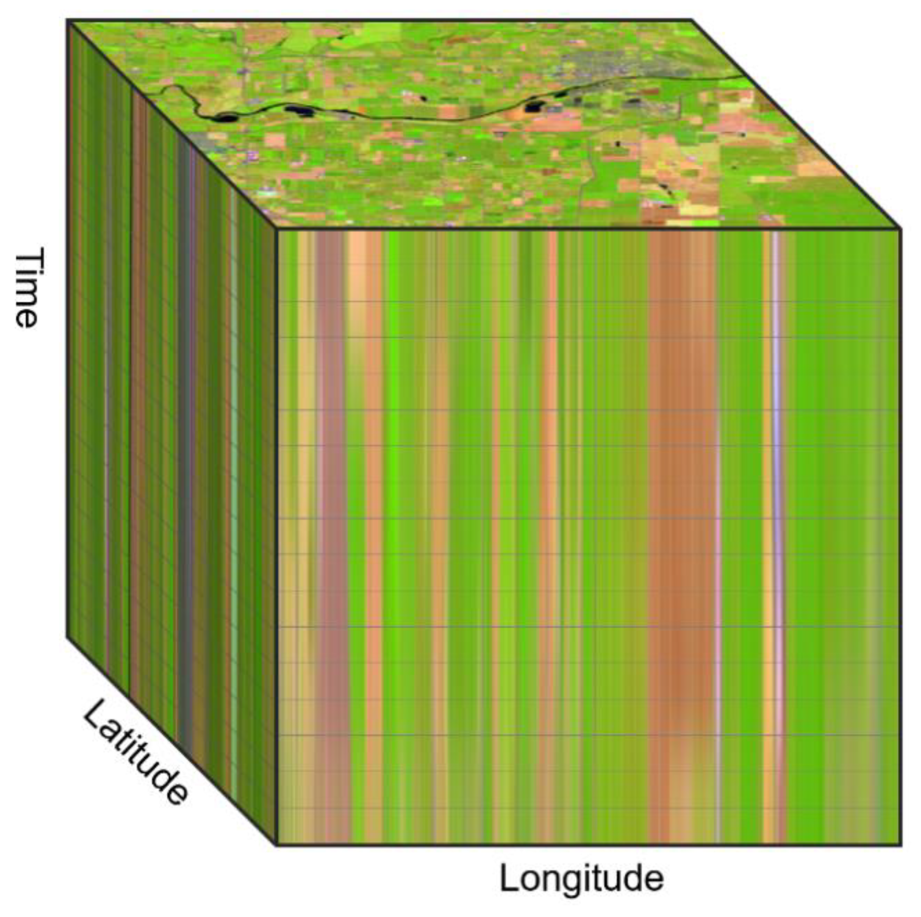
‘Data cube’ is a generic term used to describe an array of multiple dimensions. Data cubes help to organize data, simplifying data management and often improving the performance of queries and analysis. In its simplest form it can be thought of as a 3D spreadsheet where three axes may represent sales, cities, and time. In a mapping context, the two primary dimensions of a data cube are typically the latitude and longitude position. Other common dimensions of geospatial data are time, depth (when working with geologic or oceanographic data), or altitude (when working with atmospheric data). Data cubes of earth observation imagery are typically three dimensions; latitude, longitude, and time,
Figure 1.
A query of an image data cube at a specific time, will return an image map such as that seen on the top level of the cube in
Figure 1. A query of an image data cube at a specific location will return the time series of values at that location, like a vertical probe dropped on top of the cube. The cube structure also simplifies data aggregation operations such as weekly, monthly, or annual analysis.
After years of talk of democratizing geospatial data [
11] we are finally seeing notable progress [
12]. ‘Democratizing’ is not simply about making data and analysis more available, it also requires improving accessibility in a way which leads to widespread adoption and awareness. This means it is necessary to understand potential end users and provide a relevant and approachable user experience. The availability of image data cubes, cloud hosted image analysis, and web technology means this can best be accomplished through easily configurable web applications tailored to the knowledge and goal of the user.
Google Earth increased global geospatial awareness by providing access to data in a simple user experience suitable to the skills and needs of its users. Prior to this, GIS and web maps were more of a niche few people were aware of, now everyone knows how to navigate a web map. The same is possible with earth observation data and geospatial data science through the use of image data cubes and tailored web applications.
This paper describes a collection of geospatial technology components which in combination establish a complete platform for Earth observation data exploitation, from data ingestion and data management to big data analytics to sharing and dissemination of modeling results. The first section of the paper describes the technology components, their relevance toward achieving the full vision of Earth observation data cubes as well as insight to lessons learned along the way. The second section of the paper will present three application case studies applying this approach to a variety of data cubes.
2. Method
To obtain the full value of image data cubes, development and integration is required in a number of areas: data preprocessing, storage optimization, data cube integration, analysis, and sharing.
2.1. Image Preprocessing—Building Analysis Ready Data
Processing imagery before loading into a data cube structure to create Analysis Ready Data (ARD) is a foundational aspect of modern earth observation data cubes. ARD preprocessing has been described as a fundamental requirement [
13], disruptive technology [
13], and cornerstone of the Open Data Cube initiative [
10]. ARD preprocessing makes it easier for a wider audience of non-imagery experts to perform more correct analysis, thus expanding the potential number of people correctly applying earth observation imagery [
13]. There are multiple approaches and programs for ARD processing [
10,
13].
Many image processing workflows to create ARD involve resampling the pixels, which decreases their quality. While all resampling creates some artifacts, choices can be made appropriate to the application. For most scientific applications, it is desired to minimize resampling such that only one resampling takes place and the type of resampling is most applicable to the type of analysis. Where spectral fidelity is important nearest neighbor resampling is recommended, and for applications where textural fidelity is important, bicubic or similar sampling is recommended. One of the decisions in a data cube preprocessing workflow is to what sampling should be applied and how soon after the imagery is acquired should the data be processed, or if there is a need to re-process all the data when new transformation parameters are determined.
Ideally, the data would remain as sensed by the sensors and the user performing the analysis would define the geometric transforms, projection, pixel size, pixel alignment, as well as radiometric corrections to be applied to the imagery for analysis specific to their needs. This would require providing access to the source data, which increases the complexity of any analysis, and adds an unnecessary size limit on the type of problem to be solve. Hence the data cube concept requires the selection and agreement on all these factors and the data is data is preprocessed to these specifications. The intent and assumption is the data is only resampled once and all subsequent processing will be done with the defined pixel alignment.
There are multiple approaches and programs for ARD processing [
10,
13] and CEOS has developed a set of guidelines for ARD processing known as CARD4L [
14].
2.1.1. Radiometric Preprocessing
To improve analysis results, the radiometry of the sensor needs to be calibrated and corrected for a variety of sensor anomalies, as well as effects of atmosphere, for which multiple approaches are available [
13]. Determination of multiple radiometric transforms is complex and relies upon auxiliary data that may not initially be available at the time of image acquisition. What may be of sufficient accuracy for one set of scientific analysis may not be sufficient for another. Tradeoffs are evaluated, and compromises reached to determine a level of processing that is sufficient for the majority of the users based on the best available auxiliary data. For most data cube applications, the data is processed to an agreed level of surface reflectance.
In addition to correcting pixel values to surface reflectance, additional calculations are often performed to flag pixels such as cloud, and cloud shadow, which can be problematic for some analysis techniques. Cloud masks can be computationally expensive to create, and compress well for efficient storage, and therefore are frequently part of the preprocessing workflow and stored as a binary image mask.
A balance needs to be found between processing and storage. If a parameter can be computed by a computationally simple local function from the existing datasets, then it is generally better to compute this when needed instead of during preprocessing which requires additional processing and storage.
For example, computing an NDVI from two bands is computationally insignificant and would result in a new product that requires significant storage and is therefore typically not part of the preprocessing workflow. NDVI and other band indices are more often implemented as a dynamic process performed when needed, as described in
Section 2.4.1.
Geometrically referencing the pixels, computing surface reflectance, and creating cloud masks are computationally expensive and appropriate as part of the preprocessing workflow.
2.1.2. Geometric Preprocessing
From a geometric perspective, remote sensing instruments do not make measurements in predefined regular grids. Performing temporal analysis that involves multiple data sources involves resampling the data to a common coordinate system, pixel size, and pixel alignment. Unfortunately, the transforms from ground to sensor pixels are not usually accurately available as soon as the image is collected, and the transformation parameters may improve over time.
A disadvantage of storing anything but the unrectified imagery is that the data is resampled to a defined coordinate system, pixel size and alignment. A key aspect of Analysis Ready Data is to attempt to ensure that all data is sampled to the same grid. For both the Australian Data Cube and US Landsat ARD a single coordinate system was selected, and all data processed from the Level 0 data directly to the defined coordinate system. As the spatial extent of data cubes increases the selection of appropriate projection becomes more challenging. For multiple regions, a current solution is to split the world into multiple regional data cubes each of which has a suitable local coordinate system or to use UTM Zones.
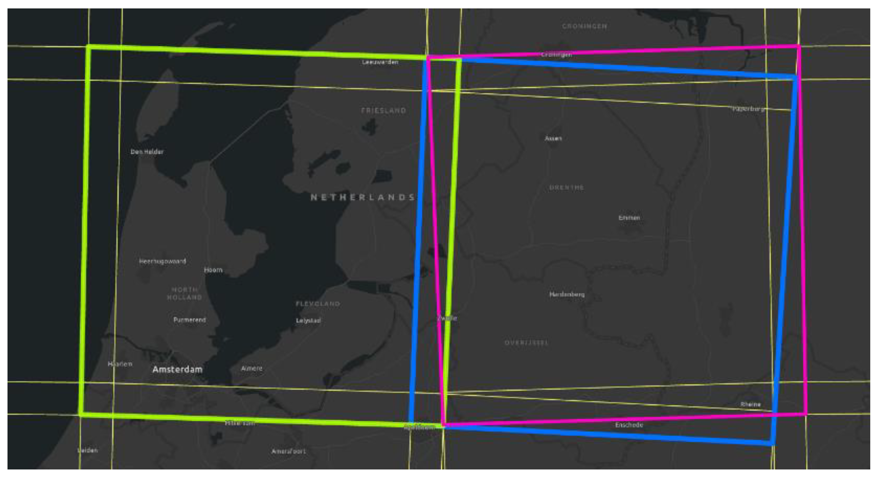
The tradeoffs in choosing an appropriate coordinate system exists for all global datasets. For Landsat and Sentinel 2 level 1 and 2 products UTM zones are being used. Each Landsat scene is defined by a unique path/row and is assigned the most suitable UTM zone. This results in pixels being aligned for all scenes allocated to the same UTM zone, but resampling is required between scenes from different UTM zones. For the Sentinel 2 scenes, each scene is cut into granules that each have their appropriate projection and data that fall at the intersection of two UTM zones is processed and stored in both projections. As the granules go towards the north and south pole there is an increasing amount of overlap and duplication,
Figure 2. Techniques have been developed [
15] for addressing the UTM zone overlap of Sentinel 2 data.
2.1.3. Tiling
The Australia data cube introduced a preprocessing step to cut all imagery into 1-degree tiles to improve parallel computation performance on their HPC hardware [
8,
16]. This step has continued into the Open Data Cube project and others. The advantage of tiling is that any pixel block or pixel location is addressed by a simple equation that defines the name and location of the file. However, because satellites do not collect data in 1-degree tiles, and the orbital track prevents collecting square areas, many more tiles are created, and many tiles are predominantly empty. To know if a pixel exists for a specific location it is not sufficient to know if a tile exists, but one needs to know the footprint of the scene or needs to read the data to determine if it is set to NoData. Hence tiling data for processing or storage reasons can noticeably increase the data access time during use.
The alternative is to maintain the data as individual scenes as acquired by the satellite, where each scene is referenced to a single file which has a corresponding footprint polygon that defines the extent of the data. For any pixel location, a simple query of the footprint polygon determines if a scene exists and has data. Such geometry queries are highly optimized and efficiently eliminate requests fetching files, blocks, or pixels which contain little or no information.
From a file structure perspective both the tiled datasets and the scene datasets are internally tiled, meaning that the pixels inside of a file are grouped into regularly size contiguous chunks so that all pixels in a defined area are stored close together speeding up data access. Such tiling schemes typically use internal tile sizes of 256 or 512 pixels along each axis.
2.2. Optimizing Data Storage
Once the data is preprocessed, how the data is stored will impact accessibility, application utility, performance, and cost. Our focus is to maximize accessibility with potentially thousands of simultaneous users, make the data useful for visualization and analysis, and to balance interactive visualization performance against infrastructure cost.
Earth observation data cubes are now growing to petabytes of data leading to potentially significant infrastructure costs. Although very fast random-access storage is available the cost for such data volumes can be prohibitively high. Currently, the best approach from a cost and reliability perspective is object storage in public commercial clouds such as Amazon AWS, Microsoft Azure, and Google Cloud. Regardless, if a data cube is terabytes in a local file server, or petabytes in a cloud system, performance of the data will be impacted by choices of file structures and compression. For the best user experience, faster is better, and there are tradeoffs to balance performance and cost.
2.2.1. Compression
One way to reduce storage cost and improve performance is to compress the imagery. File compression algorithms can be lossless (pixel values do not change), lossy (pixel values are changed to achieve greater compression) or controlled lossy (pixel values change to a maximum amount defined by the user). When imagery is used for analysis, lossless or controlled lossy compression is preferred. For visualization, where exact radiometric values are less crucial, lossy compression is typically used because of its higher compression ratio. The type of compression chosen impacts not only pixel values and size, but also storage cost, performance, and computation cost.
Deflate compression [
17] is commonly used in recent data cubes as part of Cloud Optimized GeoTIFF (COG) [
18] such as Landsat AWS and Open Data Cube. It is lossless, has relatively low compression, with the benefit of low computation cost/short time for compression and decompression.
JPEG 2000 wavelet compression used in the Sentinel AWS data cube can be used as lossless or lossy. As a lossy compression it provides greater compression than is achieved with deflate compression, however the computation required to compress and decompress the data is significantly more.
LERC (Limited Error Raster Compression) [
19] is a recent compression that can be lossless or controlled lossy and provides very efficient compression and decompression of imagery data especially higher bit depth data, such as 12 bit and more. It is our recommended compression for multispectral earth observation data cubes. Unlike other lossy compression algorithms, LERC allows the user to define a maximum amount of change that can occur to a pixel value. By setting this to slightly smaller than the precision of the data the compression maintains the required precision while maximizing the compression and performance.
Advantages of LERC include that it is 3–5 times faster than deflate for both compression and decompression, depending upon bit depth, and allows the error tolerance to be defined. When used in a lossless mode LERC typically achieves about 15% higher compression ratio (smaller file) than deflate for Landsat and Sentinel type data.
To test the performance and size of different compression algorithms and formats we selected a collection of Landsat ARD files that were less than 10% cloud and with average 20% NoData (areas outside the image with no value). These where converted using GDAL version 2.4.1 to different formats and lossless compressions. The times to create and write the files and the resulting file sizes were recoded to compare data creation times, shown in
Table 1. We also recorded time to read the full image at full resolution into memory.
2.2.2. Image Format
The format of the file storage also impacts performance and therefore cost. Common choices include JPEG 2000, netCDF, tiled GeoTIFF, COG, and MRF [
19,
20]. Each has advantages and disadvantages. JP2 provides the highest compression but requires significantly more computation. NetCDF has been used in the past but is not recommended here because the data structure is not well suited for direct access from cloud storage. Tiled GeoTIFF provides a simple to access format, that can optionally include internal or external image pyramids, but is not specifically optimized for cloud usage. Multiple compression algorithms are supported including deflate, LZW, and recently LERC. COG (cloud optimized GeoTIFF) is very similar to Tiled GeoTIFF, but assumes pyramids exist for the image and stores the pyramids at the start of the file to improve performance when browsing a zoomed-out low resolution image. However, this change can significantly increase file creation time as seen in
Table 1. File creation performance for COG can be faster than in these tests if all data restructuring is done in memory.
MRF is similar to tiled GeoTIFF, but information is structured into separate files for metadata, index, and pixel data which enables different compressions including LERC and ZenJPEG making it well suited for cloud storage of data cubes. ZenJPEG is an implementation to enable the correct storage of NoData values with JPEG for improved lossy compression at 8 or 12 bits per channel. The fact that the metadata and index is kept separately enables applications to easily fetch and cache it, thus reducing repeated requests for the information when accessing large numbers of files. All these formats are directly supported by GDAL [
21] which is used by most applications for accessing geospatial imagery.
Our tests as reported in
Table 1 found MRF with LERC compression is about 13% more compressed than COG Deflate, and MRF LERC is significantly faster to write. Reading MRF LERC is about 15% faster than COG Deflate.
2.2.3. Image Pyramids
For analysis applications at the full resolution, only the base resolution of the imagery needs to be stored. For many applications it is advantageous to enable access at reduced resolutions so that overviews of the data can be accessed quickly. This can be achieved by storing reduced resolution datasets, also referred to as pyramids, which increase storage requirements. For uncompressed data typical pyramids stored with a sampling factor of 2 would increase the storage requirements by 33%. With compressed data the additional storage requirement is a bit more due to the higher frequency of the lower resolutions. Wavelet based formats such as JP2 inherently contain reduced resolutions, but the storage is less efficient to access as described above. If storage cost is not a significant factor, storing pyramids with a factor of 2 between levels is most suitable. From an analysis perspective, the existence of reduced resolution datasets provides limited value.
Alternatives to reduce storage include skipping the first level, changing the sampling factor to 3 or using lossy compression for the reduced resolution datasets. An additional consideration is the sampling used to create the reduced resolution datasets. In most cases, simple averaging is performed between the levels, but naturally this is not appropriate for datasets that are nominal or categorical such as cloud masks.
2.2.4. Optimizing Temporal Access
Storing each captured satellite scene as a file or object per scene provides simplicity from a storage perspective but is not optimum for temporal access. To access a profile through time for a specific location requires a file to be opened for each temporal slice and band read. Retrieving a temporal profile for a stack of 10 scenes that each have 8 bands would require 80 files to be opened, which may be relatively quick. However, since one of the advantages of data cubes is to manage an extensive time series, a time series analysis on a Landsat data cube might need to open hundreds or thousands of files, not suitable for interactive data exploration using a web client drilling through a time series at a location.
Putting the data into a single file does not resolve the problem as the access pattern has an impact on efficiency. If the data is structured as slices then access for any specific slice is optimized, but in that pattern, temporal access still requires sparse requests. If the data are pixel aligned through time during the preprocessing, they can alternatively be structured into many small cubes (versus tiles). This results in faster temporal access since the data for a temporal search are stored closer together, but performance for accessing slices is reduced.
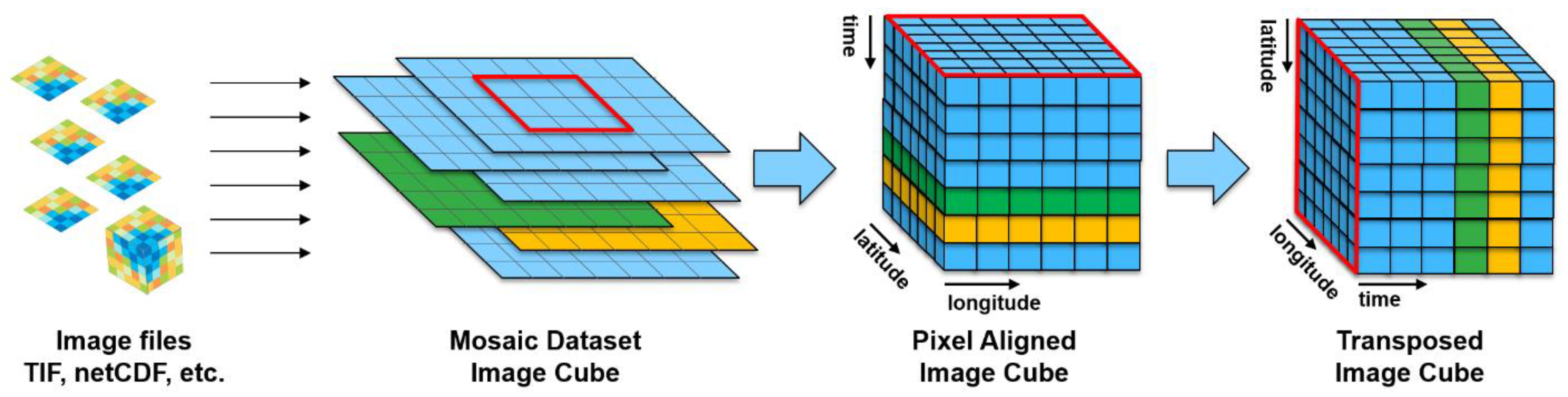
A simple approach with optimal performance when retrieving both image areas as a single time slice, and a time series at a location is to replicate the data and transpose it such that accessing pixels representing different times is equivalent to accessing pixels along a row of pixels in the non-transposed version, essentially rotating the axis of the data,
Figure 3. Although this doubles the storage volume of the full resolution data, it also maintains the best possible simultaneous performance for both query types.
An efficient balance to optimizing temporal access to a data cube is to store the data as efficiently as possible as slices (traditional scenes by date), and when repeated temporal analysis of an area of interest is required, generating a transposed data structure that is optimum for the analysis.
There are many decisions to make in designing and preprocessing a data cube. These decisions result in optimizations and compromises based on the requirements of the application and resources of the data cube creator. The result will be many different data cubes of different styles, flavors, and capabilities. The following sections address how these different data cubes can be seamlessly integrated into a platform for visualization and analysis.
2.3. Building and Referencing Image Data Cubes
A mosaic dataset [
22] is an ArcGIS data structure which holds metadata about images, a pointer to the image pixels, as well as processing workflows to be executed when the pixels are accessed. The mosaic dataset is how ArcGIS builds and manages data cubes, as well as the mechanism for integrating third party data cubes such as those described in
Section 3 of this paper.
Mosaic datasets do not store pixels, but instead the pixel data remains in its original or most appropriate form and is referenced by the mosaic datasets. The mosaic dataset ingests and structures all the metadata and stores it as a relational database such as a file geodatabase or any enterprise database such as Postgres or SQL Server, as well as cloud optimized databases such as AWS RDS Aurora. This enables high scalability and allows the mosaic dataset to be updated while in use.
The mosaic dataset can also store processing rules to transform stored pixels into required products, such as a pansharpened image, or a variety of band indices such as vegetation, water, etc.
The processing is defined by function chains that can include both geometric and radiometric transformations of the data. In a simple case, a mosaic dataset may consists of a collection of preprocessed orthoimages in a single coordinate system, or could be a collection of preprocessed orthoimages in a variety of coordinate systems projections which are reprojected on the fly when the data is requested. The processing chains can be complex, for example a mosaic dataset may reference imagery directly acquired by a sensor and the processing chains can define both geometric transformations (such as orthorectification to a defined digital terrain model) and radiometric transforms (such as to convert sensor data into surface reflectance). Mosaic datasets can be created using a wide range of tools within ArcGIS including dialogs, graphical model workflows, Python scripts, and Jupyter notebooks.
To simplify the user experience with common image data sources, Esri works with satellite and camera vendors to create definitions of how to recognize and read particular sensor data, include appropriate metadata, and how to process it. For example, if a user runs an NDVI function on Landsat 5 data, it knows the appropriate spectral bands to use without requiring the user to specify which bands contain red and near infrared information. This sensor metadata and processing information is stored as a raster type definition [
23]. ArcGIS includes a wide range of raster types supporting many data products from DigitalGlobe and Airbus as well as USGS. MTL for Landsat and Dimap for ESA Sentinel 1 and 2, and more. New raster types can be easily created by users in Python to ingest metadata and define processing for any structured pixel data. Custom Python raster types are how ArcGIS is taught to read metadata and pixels from Digital Earth Australia and Open Data Cube YAML files, and the other examples later in this paper.
2.4. Analysis
ArcGIS provides two types of analysis on imagery: dynamic or on-the-fly analysis performed at the current display extent and resolution, and raster analytics typically performed at full resolution analysis with persistent results.
2.4.1. Dynamic Image Analysis
Dynamic image analysis is the most common approach for interactive data exploration, rapid prototyping of analysis, or creating highly interactive web applications for exploring data cubes and performing computationally simple analysis. It is most suitable for local (per-cell) and focal (neighborhood) operations, and supports function chaining to allow multiple operations to be performed in a single step. This is done as a single operation with no intermediate files created. When the map is zoomed or panned the calculation is recomputed for the new area and result displayed, with no noticeable performance difference between this computation and simply drawing a band combination with no calculation.
There are over 150 raster functions provided, covering a wide range of image processing and analysis capabilities, a graphical editor for constructing function chains, as well as the ability to author custom raster functions with Python. For overlapping imagery, the system can provide a single output by blending the pixels, aggregating, or computing a variety of statistics per pixel location. To extend the provided functions the system can return and utilize a Python NumPy, XArray, or ZArray for integration with a wide range of scientific analysis libraries.
Processing workflows can be defined in advance as part of the mosaic dataset definition, and also controlled or modified as desired by a client application. For example, a web application can expose multiple decades of imagery, a variety of band index options, and a change detection tool, which allows an end user to select a band index of interest and dates of interest, e.g. to find areas with a significant change in vegetation, the server would compute NDVI for each of two dates, compute the change, and apply a threshold and colormap to the result. Due to the way the imagery is stored and served, such a calculation can return a result dynamically as the map is panned, zoomed, or a different or band index is chosen.
2.4.2. Big Data Image Analysis
Although dynamic image services provide an excellent experience for performing on-the-fly processing they are not optimum when processing a large extent at high resolution. To perform more rigorous analysis, such as segmentation and classification, or create persistent results we developed a distributed computation framework for local, focal, and global analysis, which automatically chunks and scales to the to the number of processes requested by the user. The system scales efficiently from a small number of parallel processes on a local machine to hundreds of processes in a distributed cluster, and can utilize GPUs when available. To perform analysis on data cubes, we developed efficient search, parallel read/write, and distributed computation capabilities, which can be deployed to an on-premise private cluster, or in commercial cloud such as Amazon or Azure. The system includes the same analysis capabilities as the dynamic image services described above, plus highly optimized versions of more complex analysis such as segmentation, classification, shortest path, terrain and hydrologic analysis. The system also integrates with third party analytic packages through Python, R, CNTK, TensorFlow, and more. These optimized algorithms working on massive distributed data in publicly accessible cloud storage allowing anyone to perform analysis which previously would be performed on a supercomputer.
Many image processing tasks are computationally simple and can become I/O bound in a parallel compute setting. To illustrate the effectiveness of parallel I/O capabilities of the system we ran an image processing workflow on the Landsat GLS 1990 collection. The data was 7422 multispectral scenes stored in Amazon S3. The analysis workflow was for each scene to generate a NoData mask, perform a top of atmosphere correction, calculate a modified soil adjusted vegetation index, slice this into categories, and write the output image. The computation was performed on a single node, 32 core AWS c3.8XLarge with 60gb of RAM. We ran 200 processes against the 32 cores and the task completed in 2 h and 48 min averaging approximately 44 scenes per minute.
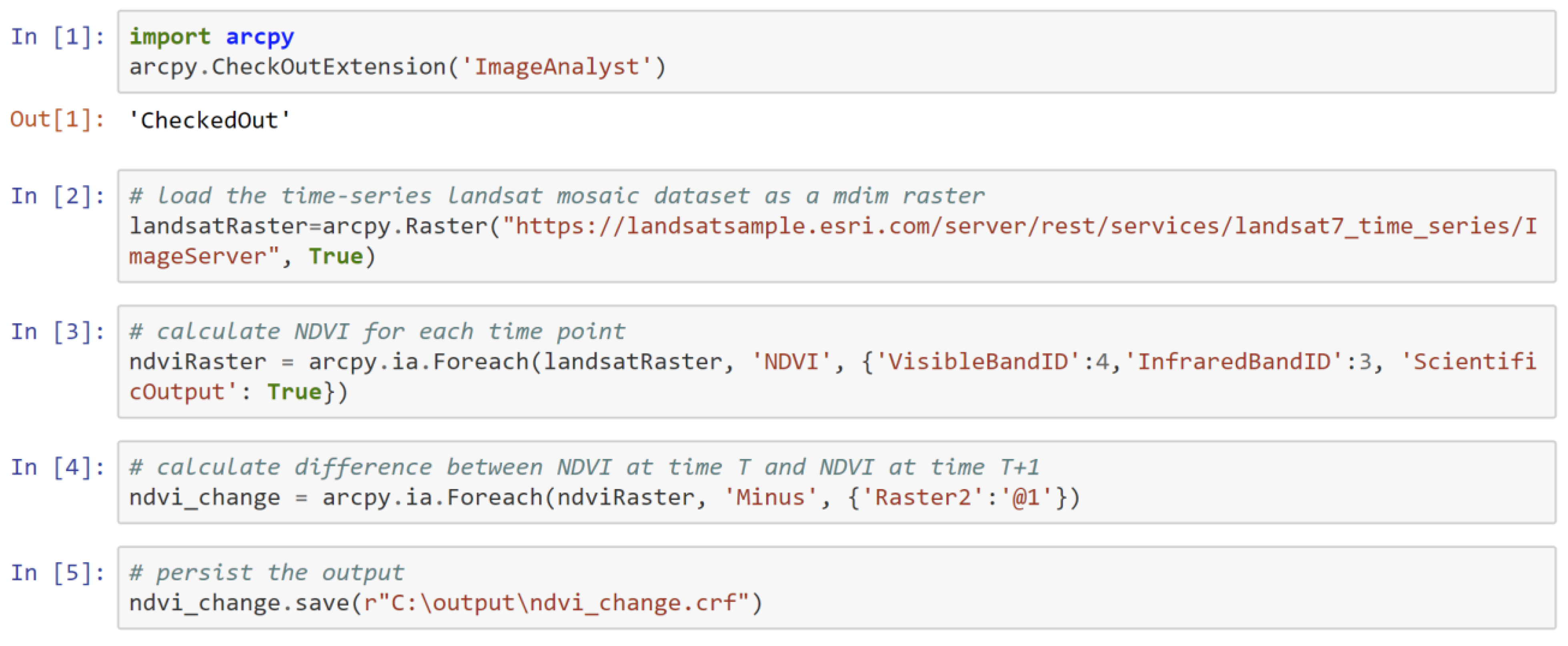
For large computation-intensive workflows, it is helpful to distribute the compute load over multiple nodes in a cluster, each with multiple cores. New algorithms were architected and developed to scale efficiently in a distributed compute environment where the software framework automatically chunks and distributes work to each node and core. The input data for this test was a 397 gb, 1-meter resolution area of the National Agriculture Imagery Program (NAIP), approximately 100 billion pixels. The analysis workflow performed was a mean shift segmentation, classification, and write the output file. The computation was performed on a 10 node x 20 cores each Azure Standard_DS15_v2 with 140 gb of RAM. We ran 200 processes and the task completed in 1 hour and 13 min. A Python example of a similar workflow is shown in
Figure 4.
Big data analysis workflows can be authored in ArcGIS Pro and run locally or in a remote cloud server. Because the underlying tools and APIs are the same, the only difference between running on a local desktop and in a remote cloud server is one parameter on the dialog. It is similarly easy to publish that workflow to the server so others can access it. Analysis workflows can be authored from dialogs, graphical modelers, Python, and Jupyter notebooks,
Figure 5. Published services are available via REST and OGC protocols.
2.5. Sharing the Value of Image Data Cubes
To achieve the vision of expanding the use of imagery and increasing its impact it is necessary to grow the community of people using and understanding imagery. This can be achieved through web services and web applications.
2.5.1. Sharing Web Maps and Image Services
Web services define a protocol for two pieces of software to communicate through the internet, for example for data from one server to appear as a map in a client application. Imagery can be served with a variety of protocols [
24,
25] including OGC WMS, OGC WCS, REST, etc. Map services such as OGC WMS are the most common way to serve imagery and is essentially a prebuilt picture of the data. It is most useful as a background image when used with other data in a web map but is of limited value for data exploration and analysis because the original data values are often not available. For example, if provided as jpeg which is lossy compressed, or the data is higher than 8-bit pixel values and needs be rescaled to fit into an 8-bit RGB PNG. However, because the display has been predefined, map services are the easiest to use for an imagery novice who does not understand bit depth and stretching values for display, or edge effects of multi-date imagery.
Image services support interactive image exploration and analysis, and are a cornerstone of image analysis on the web. They are commonly published as REST, SOAP, or OGC WCS. Image services provide web applications access to original pixel values, and all bands and dates the publisher chooses to share. Image services can support a wide range of dynamic image analysis and exploration described above in
Section 2.4.1, as well as full resolution analysis described in
Section 2.4.2, as well as extraction for download.
2.5.2. Sharing Analysis
To increase the impact of imagery it should be transformed from data to information through some analytic workflow. There are a variety of ways to share analysis tasks and workflows to enable non-experts to be able to extract useful and reliable information from imagery. Analysis workflows can be defined as part of a mosaic dataset and published as part of the image service, and when accessed by a client application the analytic workflow is executed dynamically. Analytic workflows can also be published as geoprocessing services, OGC WPS, Python scripts, and as Jupyter notebooks. Using analytic web services, applications can combine data and analysis from multiple locations to solve a unique new task possibly not envisioned by the service publisher. For example, combining a fire burn scar difference image analysis service from one publisher with a population overlay service from another publisher to compute the number of people impacted by a fire.
ArcGIS image analysis workflows are most often authored in ArcGIS Pro, which was designed from inception to be well integrated for publishing and consuming cloud-based web services. Workflows are designed using dynamic analysis for rapid prototyping, and then shared to the cloud for scaled up big data analytics at full resolution, which can be accessed by any web client application, including ArcGIS Pro.
2.5.3. Web Applications for Focused Analytic Solutions
Providing a relevant and approachable user experience to the breath of potential users and skill levels is best accomplished through configurable web applications tailored to the knowledge and goal of the end user. The web applications are powered by cloud hosted analysis services and image services published from image data cubes.
Web applications can be created that access all forms of geospatial web services. Applications consume predefined services and can also interact with the dynamic services defining the processing to be applied. Users can also compose new workflows through web applications. Such processing can be on-the-fly processing or can also include running analysis tools that interact with cloud servers performing large computation tasks. These web applications not only act as clients to servers, but can also retrieve the data values for the servers enabling the creation of highly interactive user environments that make use of the processing capabilities available in modern web browsers.
With the emergence of cloud technology, we have seen the continuous growth of Software as a Service [
26]. Esri’s SaaS solution, ArcGIS Online, is part of the overall ArcGIS platform, designed to work seamlessly with ArcGIS Pro and is included with all ArcGIS licenses. It provides access to petabytes of geospatial data and hosted analytic services, as well as providing infrastructure for hosting users’ data and all types of geospatial services including image services and analysis services. It also includes capabilities to author and host custom web applications. Applications can be written using in Javascript, or using a drag and drop user interface such as Web AppBuilder. For imagery services there are a collection of prebuilt web control widgets including spectral profile, time series profile, scatterplot, change detection, and more. Configurable web application templates are also provided for common web application needs such as image change detection and interactively browsing image time series. Using a web application template a novice can progress from a web map to a fully hosted and publicly accessible web application in minutes.
It is now easy enough to build custom web applications integrating image services and image analytics that almost anyone can create an interactive application to share specific data, analysis, and stories. It is no longer necessary for a stakeholder or executive to navigate a generic geospatial software to understand a drought or zoning problem, their staff familiar with the data and analysis can create and share a simple web application to lead them through understanding the problem in a way that is relevant to their knowledge and needs. Representative of their ease and popularity, there are currently over 3 million web applications in ArcGIS Online, with approximately 1000 new Web AppBuilder applications created each day.
3. Results
3.1. Landsat and Sentinel in Amazon
In 2015 Amazon Web Services in collaboration with USGS and the assistance of Planet began loading Landsat 8 Level-1 data into an Amazon S3 bucket and provided open public access [
27]. Using the raster type and mosaic dataset approach described in
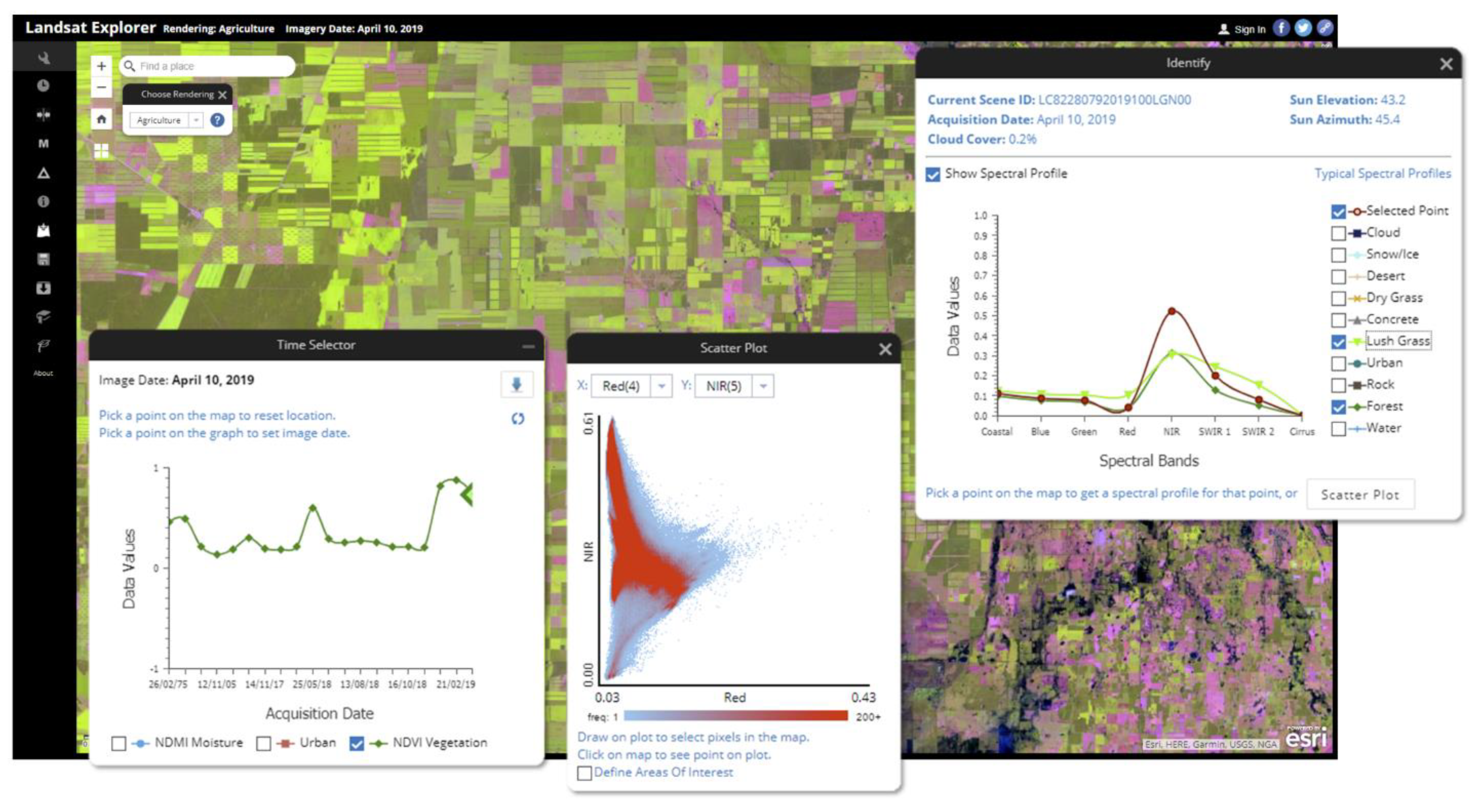
Section 2, Esri provides visualization and analysis of this data through a free, easy to use web client,
Figure 6, as well as web service access for visualization and analysis in other applications.
Whereas the traditional approach to an image archive would start with first searching and selecting individual scenes to view, these services and web application provide an interface that enable users to pan and zoom to any location on earth and see the best available Landsat scenes in a wide range of different band combinations and enhancements. The web client also allows searching based on geographic extent, date, cloud cover, and other criteria. A timeline slider control is used to refine the date selection.
The application supports a variety of interactive analyses from common band indices for evaluating vegetation, water, and burn scares, as well as image thresholding and change detection. All image processing functions are applied on the fly by the server using the dynamic processing capabilities described in
Section 2. The application also includes graphing widgets for exploring spectral signatures of areas, or of individual locations through time,
Figure 6. With a few clicks, anyone with internet access can examine vegetation health through time, and map burn scars or water bodies, anywhere in the world.
A more traditional approach to Landsat data would be to search for individual images, download images to a local desktop computer, then use a desktop image analysis software application to process the data, all of which requires more skill, and significantly more time.
Since the initial release, the Landsat collection in Amazon has grown to over a million scenes. Each day new scenes are added to the collection and an automated script updates the mosaic dataset referencing the scenes, making new imagery available as image services accessible to client applications. Python scripts are triggered as new scenes become available and use a raster type to read the metadata from USGS. MTL files to set up the appropriate functions in the mosaic datasets. The resulting mosaic dataset defines a virtual data cube that can then be accessed for analysis or served as dynamic image services.
The application and services are deployed on scalable commercial cloud infrastructure, allowing them to grow with demand over the last 4 years. They now regularly handle tens of thousands of requests per hour and maintain response times suitable for interactive web application use.
In 2018, Esri developed similar web services to access and share the Sentinel 2 available from the AWS Open Data registry [
29]. These services use similar scripts that automate the ingestion of the metadata into the mosaic datasets from the Sentinel 2 DIMAP files. It can be accessed via a corresponding Sentinel Explorer web application [
30].
These Landsat and Sentinel 2 services are also available in a single Earth Observation Explorer application [
31]. It provides access to both collections in a single application and allows easy side-by-side comparisons of proximal image dates from different sensors, providing useful insight when used with the interactive image swipe tool.
3.2. Digital Earth Australia
The Australian GeoScience Data Cube was developed by Geoscience Australia and hosted on the National Computing Infrastructure at Australia National University. It was a 25-meter resolution, pixel aligned collection of over 300,000 Landsat scenes which were geometrically and spectrally calibrated to surface reflectance [
8,
16]. This was the first continental Landsat data cube with a large number of overlapping scenes in time, enabling new types of analysis to be envisioned and developed. A new version of this data cube has been created and is now known as Digital Earth Australia (DEA).
Geoscience Australia replicated the DEA cube in Amazon S3 and provided access to Esri Australia to prototype a capability serving DEA data from S3 using ArcGIS Image Server to enable hosted visualization and analysis from external client applications. The DEA data cube utilizes a YAML file to store metadata about each image tile. A Python raster type was created to allow the system to parse the YAML file of the data cube to generate an Esri mosaic dataset which holds the metadata and references to images stored in the cloud. The mosaic dataset makes all the imagery and metadata easily accessible through multiple APIs, directly in desktop applications or through image services published from ArcGIS Image Server, and therefore web clients.
This prototype also developed server-side analytics for common DEA data products such as Water Observations from Space (WOfS) [
32]
Figure 7. WOfS is a relevant test case because it benefits from the data preprocessing such as surface reflectance calibration and pixel alignment that is part of the data cube construction preprocessing. The analysis runs in Amazon near the DEA imagery. These calculations can be computed on-the-fly for the current display extent and resolution, or at full resolution to a persistent output dataset using a distributed computation service. Data visualization and analytics were shown to be accessible and responsive through Javascript web clients and ArcGIS Pro. Additional analytics and web applications are being considered for future development.
3.3. Digital Earth Africa
The Open Data Cube [
9] is a NASA-CEOS initiative in collaboration with Geoscience Australia to create open source software for creating, managing, and analyzing Earth observation data cubes. The largest project is a data cube for the continent of Africa known as Digital Earth Africa. The initial prototype of this project was the Africa Regional Data Cube (ARDC) created in 2018 which covers Kenya, Senegal, Sierra Leone, Ghana, and Tanzania [
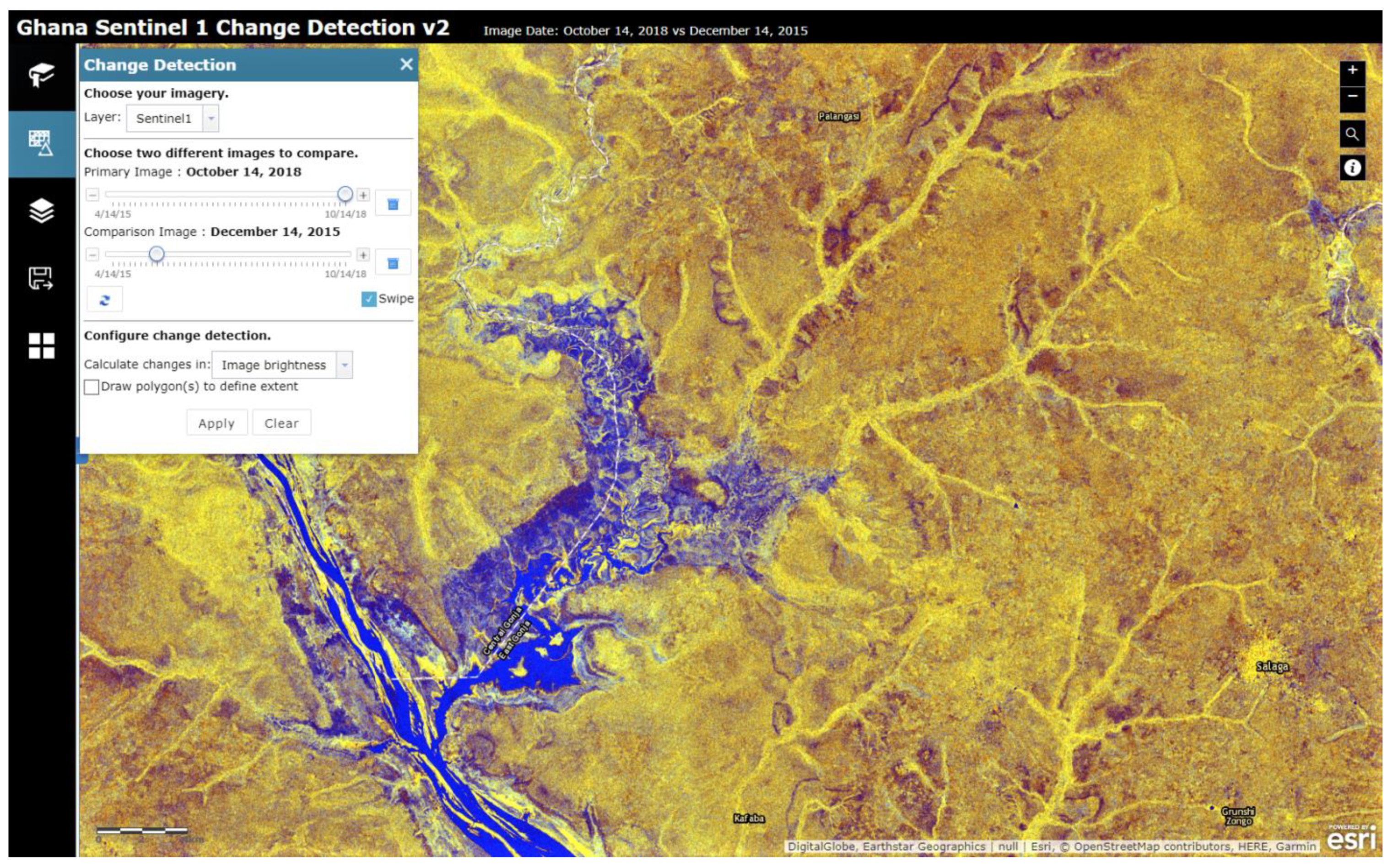
10]. NASA-CEOS provided access to the image data cube of Ghana stored in Amazon S3, which contains Landsat and Sentinel 1 data. The Sentinel 1 data is a collection of 44 monthly mosaics created by Norwegian Research Centre (NORCE).
Building upon experience gained from the Digital Earth Australia collaboration described above, the Python raster type for reading the YAML files was modified for the characteristics of the Africa data collections and a mosaic dataset created to reference the images.
A collection of image services and web applications were published for exploring spectral indices through time, as well as performing interactive change detection of spectral and radar data,
Figure 8. Additional analytic workflows are under development. This ongoing collaborative research and prototyping exercise is developing Python workflows and tools to publish similar open capabilities from the Digital Earth Africa data cube when it becomes available.
The image services, analytic services, and web applications will be made openly accessible through the Africa GeoPortal [
33], a no-cost open portal for geospatial data and applications in Africa. The Africa GeoPortal is a fully cloud hosted SaaS, enabling users to create and share their own data, web maps, analysis, and custom hosted web applications. These open services and applications for Africa will be included into the search of other geospatial portals such as ArcGIS Online, which is part of the federated search of the GEOSS Portal and others supporting the appropriate OGC web service standards.
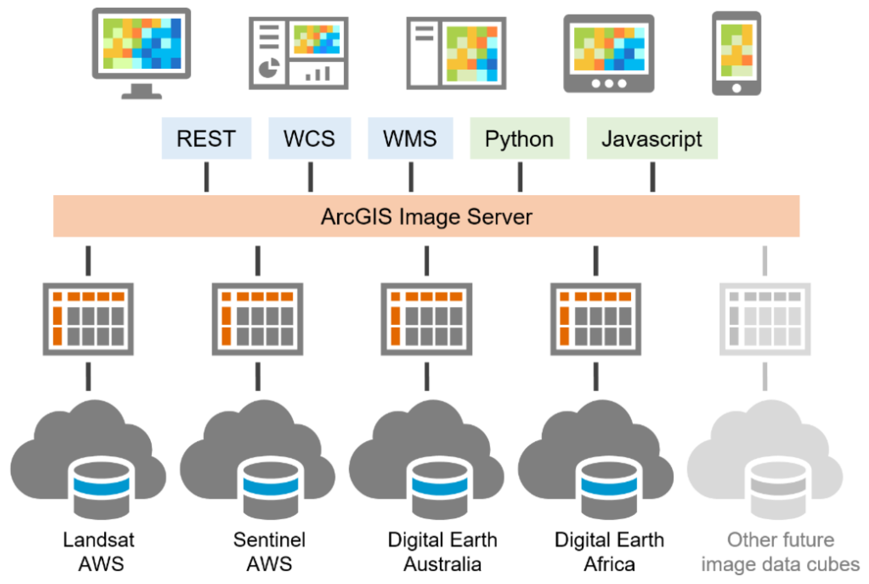
The three use cases described above use a common approach and software platform for accessing, analyzing, and sharing imagery from four different image data cubes. These data collections were built by four different groups of people in different locations, using different formats, compression, coordinate systems, and tiling schemes. The data is hosted on three different continents, yet is accessible from any internet connection through easy to use web applications and standard APIs,
Figure 9. All applications presented maintain response times suitable for interactive exploration and analysis through web applications, and required no data download or image replication. Interested readers are encouraged to visit the Earth Observation Explorer application [
31] for their area of interest. This approach is applicable to nearly any spatially and temporally organized collection of earth observation imagery.
4. Conclusions
We described here a platform for accessing, analyzing, and sharing earth observation imagery from a variety of data cubes. Free and low-cost open data sharing and cloud hosting of large collections of imagery as data cubes is improving access and increasing usage of earth observation data. ARD preprocessing is an important and beneficial step in building data cubes but includes compromises that should be understood by data cube creators. Cloud hosted image analysis transforms image data into actionable information, increasing its value and potential for impact. Analytic web applications tailored to specific stakeholders and problems are growing in use and make multispectral and multitemporal imagery more approachable to a larger audience.
Within the next 5 years, we expect that nearly all earth observation data will exist in some form of ARD image data cube hosted in the cloud and provide hosted analytic web services. Therefore, it is important that software be capable of efficiently accessing and using data without replication from the variety of data cubes which will be created.
All python scripts, custom raster types, and sample applications developed for and described in this paper are freely available as examples to follow for anyone interested in connecting to or building other similar data cube integrations. New online training materials for how to build and integrate data cubes are being developed, as well as new training materials [
34] illustrating how to use image data cubes and other data for addressing United Nations Sustainable Development Goals.


