Data Descriptor

A Rainfall Data Intercomparison Dataset of RADKLIM, RADOLAN, and Rain Gauge Data for Germany

1
Institute of Physical Geography and Landscape Ecology, Leibniz Universität Hannover, Schneiderberg 50, 30167 Hannover, Germany
2
Institute of Bio- and Geosciences IBG-3, Forschungszentrum Jülich GmbH, 52425 Jülich, Germany
3
Leibniz Centre for Agricultural Landscape Research ZALF, Eberswalder Straße 84, 15374 Müncheberg, Germany
*
Author to whom correspondence should be addressed.
Data 2019, 4(3), 118; https://doi.org/10.3390/data4030118
Submission received: 29 June 2019 / Revised: 23 July 2019 / Accepted: 29 July 2019 / Published: 2 August 2019

Abstract

:
Quantitative precipitation estimates (QPE) derived from weather radars provide spatially and temporally highly resolved rainfall data. However, they are also subject to systematic and random bias and various potential uncertainties and therefore require thorough quality checks before usage. The dataset described in this paper is a collection of precipitation statistics calculated from the hourly nationwide German RADKLIM and RADOLAN QPEs provided by the German Weather Service (Deutscher Wetterdienst (DWD)), which were combined with rainfall statistics derived from rain gauge data for intercomparison. Moreover, additional information on parameters that can potentially influence radar data quality, such as the height above sea level, information on wind energy plants and the distance to the next radar station, were included in the dataset. The resulting two point shapefiles are readable with all common GIS and constitutes a spatially highly resolved rainfall statistics geodataset for the period 2006 to 2017, which can be used for statistical rainfall analyses or for the derivation of model inputs. Furthermore, the publication of this data collection has the potential to benefit other users who intend to use precipitation data for any purpose in Germany and to identify the rainfall dataset that is best suited for their application by a straightforward comparison of three rainfall datasets without any tedious data processing and georeferencing.
Dataset: Available at Zenodo data repository, DOI:10.5281/zenodo.3262172. (https://zenodo.org/record/3262172)
Dataset License: CC-BY-SA 4.0

1. Summary

Rainfall is a major driver for many environmental processes. The operational monitoring and management of water resources as well as the modeling of many water-related processes require spatially and temporally highly resolved rainfall data [1].
Weather radar systems can provide such highly resolved data, but due to the indirect measurement technique, radar data are also subject to systematic and random bias and various potential uncertainties. In the last two decades, much progress has been achieved in the derivation of quantitative precipitation estimates (QPE) from weather radar reflectivity data through the development of new algorithms. These led to improvements in reflectivity data correction (removal of clutter, e.g., due to wind energy plants, ground echoes, attenuation correction, detection of spokes and erroneous bright band echoes, etc.), conversion from reflectivity to precipitation heights, adjustment to rain gauge data and the creation of gridded composites from the local radar station data (e.g., [2,3,4,5,6,7]).
In Germany, the operational RADOLAN (“Radar Online Adjustment”) program was launched by the German Weather Service (Deutscher Wetterdienst (DWD)) in June 2005 [8,9]. It provides hourly radar-based QPEs adjusted to rain gauge data on a nationwide 1 km grid (called RW product) as well as unadjusted QPEs with temporal resolutions up to 5 min. Though these RADOLAN composite data are a considerable improvement for spatially and temporally highly resolved rainfall monitoring, the QPEs still contain systematic errors and significant clutter. Moreover, data processing and correction algorithms as well as the radar hardware have been continuously developed since the launch of the program, which is why the RADOLAN dataset constitutes an inhomogeneous time series [10]. The data are mainly used for rainfall monitoring and operational water management and warning procedures, whereas they are still rather sparsely used in scientific research.
In 2018, the DWD published a reanalysis of all their radar data back to the year 2001 using consistent processing techniques, several new correction algorithms, and more rain gauges for adjustment. This radar climatology dataset called RADKLIM has been developed with the intent to enable radar-based climatological research and especially heavy rainfall analyses [10]. Besides hourly gauge-adjusted QPEs (are also called RW) [11], the radar climatology also comprises quasi-adjusted QPEs in a 5-minute resolution called YW [12].
The dataset described in this paper is a collection of precipitation statistics we calculated from the hourly nationwide RADKLIM and RADOLAN RW products which were combined with rainfall statistics we derived from DWD rain gauge data for intercomparison. The precipitation statistics include annual precipitation sums for the years 2006 to 2017, mean annual sums, mean seasonal sums per hydrologic half-year, the number and mean rainfall height of days exceeding a daily precipitation amount of 1 mm and 20 mm sub-divided by half-years, the number of NoData values, and several additional information on parameters that can potentially influence radar data quality. These include the height above sea level, the number, average height and diameter of wind energy plants per pixel and the distance to the next radar.
The rainfall data intercomparison dataset is shared via two vector format point shapefiles collected in a zip archive hosted at Zenodo data repository. The dataset was collected and is currently being analyzed as part of a study aimed at the evaluation of the German radar climatology. The publication of this data collection has the potential to benefit others who intend to use precipitation data for any purpose in Germany and who need to know which rainfall dataset is best suited for their analysis period and study area. The quality and completeness of precipitation datasets differs in time and space due to missing or erroneous data, changes or gaps in the network of measuring devices as well as seasonal and environmental influences such as topography, temperature or origin and type of precipitation. With a range of different datasets available (which also include satellite-based and spatially interpolated precipitation data not considered in this data collection), researchers often need to identify the best suited rainfall dataset for their application, which may be a time-consuming task that already involves a significant amount of data processing. The dataset presented in this paper can help researchers make a decision by providing a straightforward comparison of three rainfall datasets without any tedious raw data processing and georeferencing. Though, when evaluating the datasets against each other, it has to be considered that they are not independent. Most or probably all of the DWD gauge data have been used for radar data adjustment, while RADOLAN and RADKLIM share the same reflectivity measurements and some of their processing and correction algorithms. However, the rainfall data intercomparison dataset can be used to evaluate the quality of the radar data products by analyzing their spatial and temporal distribution in any individual study area within Germany and by comparison with the additional collected information. This way, it is possible to describe and assess the spatially and temporally varying radar data quality regarding the reflectivity and the applied conversions, corrections and gauge adjustment. Thus, the dataset presented in this paper can help to build confidence for using radar data or also support the decision not to use them due to data quality issues in the respective study area. Furthermore, it also constitutes a spatially highly resolved rainfall statistics geodataset for the period 2006 to 2017, which can be used for statistical rainfall analyses or to derive model inputs.
The generated dataset is described in Section 2, and in Section 3, information on the original input data sources, a detailed description of the data processing, the calculated precipitation statistics and additional parameters, as well as an evaluation on the quality and completeness of the dataset are provided. Finally, in Section 4, further notes on the usage of the dataset and a brief application example are provided.

2. Data Description

The generated rainfall data intercomparison dataset described in this paper consists of two vector format point shapefiles, which can be read by all common Geographic Information Systems (GIS). The spatial extent of both files covers the area of the Federal Republic of Germany and the temporal period ranges from 2006 to 2017.
The dataset comprises the following shapefiles radar_comparison.shp and gauge_comparison.shp.
  • Radar_comparison.shp: Point data of the centroids of the RADKLIM data grid (1 km resolution) clipped to Germany. The spatial reference is a polar-stereographic projected Cartesian coordinate system defined by DWD for their radar composite products (see [13] for more details on this custom projection referred to as ‘radar projection’ throughout this paper). This file is subsequently referred to as ‘RADKLIM and RADOLAN radar precipitation dataset’ or ‘radar shapefile’.
  • Gauge_comparison.shp: Point data of rain gauges with the geographic coordinate system WGS 84 as a spatial reference. This shapefile is subsequently referred to as ‘rain gauge precipitation dataset’ or ‘rain gauge shapefile’.
The objective of the data collection was to provide an easy-to-use dataset that enables also nonspecialists from different communities (geosciences, hydrology, meteorology, and environmental planning) to get quick insights into the properties of the radar datasets and, thus, to help improve the usability of RADKLIM and RADOLAN. Consequently, the dataset was published in the widespread shapefile geodata format in order to provide all collected information in one attribute table and enable an easy and straightforward usage in all common GIS as well as data exports to other tabular data formats. Both shapefiles contain a variety of attribute fields including a series of aggregated rainfall statistics calculated from all three precipitation datasets for comparison as well as metadata on gauge and radar pixel ID numbers, height above sea level, and some dataset-specific metadata such as distance to next radar, full gauge station names, and gauge measurement periods.
A summary of the most important attribute fields of the dataset is provided in Table 1 and the entire list of attribute fields is included in the metadata description [14].

3. Materials and Methods

In the following sections, input data sources and data availability are explained, data processing, data aggregation, and validation procedures are also described for each input dataset, and, finally, an explanation of the merging procedure applied to obtain the resulting dataset is provided.

3.1. RADKLIM and RADOLAN Radar Precipitation Dataset

3.1.1. Data Sources and Accessibility

The data basis for the radar shapefile consists of the following freely available datasets.
(a)
The hourly RADOLAN RW composite
(b)
The hourly RADKLIM RW composite
(c)
A Shuttle Radar Topography Mission (SRTM) Digital Elevation Model
(d)
A dataset on the distribution and properties of wind energy plants
(a) The RADOLAN RW dataset intended for operational, near real-time rainfall monitoring contains hourly precipitation heights for Germany adjusted to rain gauge measurements on a 900 km * 900 km grid. The product code “RW” refers to the final, hourly-resolved result of the RADOLAN radar data processing chain which includes the conversion from reflectivity to precipitation heights, various correction algorithms (e.g., for clutter and orographic beam blockage), the merging of local radar station data to a nationwide gridded composite, as well as the adjustment to rain gauge measurements using a weighted average of radar-gauge differences and ratios. The RADOLAN RW product is available at the DWD Climate Data Centre (ftp://ftp-cdc.dwd.de/pub/CDC/grids_germany/hourly/radolan/historical/bin/) and covers the period from June 2005 until now, with the most recent file being provided ~20 min after the end of the last measurement interval. For comparability with the other datasets, the period 2006 – 2017 was used for the dataset presented in this paper. RADOLAN data are provided in a custom binary format with one file per hourly composite, which are collected in monthly zip archives. Additional information on data format, projection and radar locations is provided in the accompanying project report and file format description [8,15].
(b) The RADKLIM RW dataset [11] which is available at the DWD Open Data Portal (https://opendata.dwd.de/climate_environment/CDC/grids_germany/hourly/radolan/reproc/2017_002/bin/) contains hourly precipitation heights for Germany adjusted to rain gauge measurements on a 1100 km * 900 km grid. This radar-based precipitation climatology dataset is a reanalyzed and temporally extended version of RADOLAN using consistent processing techniques, several new correction algorithms (e.g., for distance- and height-dependent signal reduction and for spokes) and more rain gauges for adjustment. The dataset currently covers the period of 2001 to 2017, but only the years from 2006 onwards have been used for the dataset presented in this paper in order to allow for a comparison to the shorter RADOLAN time series. The file format is similar to RADOLAN, except for the extended grid size and the files containing more header information.
(c) The Digital Elevation Model (DEM) derived by the Shuttle Radar Topography Mission (SRTM) contains the height above sea level in meters with a grid resolution of 25 meters and is freely available for researchers at the EOWEB Geo Portal (https://geoservice.dlr.de/egp/).
(d) The wind energy dataset contains information on the spatial distribution and properties of wind energy plants in Germany. It is part of a renewable energy dataset collected by [16] and provided in shapefile format by the Helmholtz Centre for Environmental Research (Umweltforschungszentrum, UFZ) (https://www.ufz.de/record/dmp/archive/5467/de/). Information on wind energy plants was included in the dataset since they may cause false echoes and, thus, clutter and noise in the radar measurements.

3.1.2. Data Processing, Aggregation, and Validation

Step 1: RADKLIM and RADOLAN raw data processing
Using the Python package radproc [17], the raw RADOLAN and RADKLIM datasets were both unzipped separately, clipped to the Federal Republic of Germany, imported into monthly pandas DataFrames [18] with one column per radar pixel and one row per hour and saved to two identically structured HDF5 files [19] with one group per year and therein twelve monthly datasets.
During this process, so-called ID rasters with the locations of the numbered data pixels were generated, one raster for the 900 km * 900 km RADOLAN grid and one for the 1100 km * 900 km RADKLIM grid. The ID rasters are clipped to Germany and used as a basis for the raw precipitation data clipping and for the subsequent export of results to raster datasets. A more detailed description of the raw data processing methodology is provided by [20].
Step 2: Calculation of precipitation statistics
The calculations for all precipitation statistics are based on the generated HDF5 file and functions from the Python packages radproc, pandas, and numpy [21]. Most of the calculated statistics are self-explaining or comprehensively outlined in Table 1 and the metadata description (e.g., precipitation sums per year or hydrological half-year and number of days exceeding a precipitation sum of 1 mm or 20 mm), which is why the following sections are limited to describing data cleaning and validation approaches as well as some dataset-specific parameters.
The calculated mean annual precipitation sums showed significant differences between RADKLIM and RADOLAN with much higher values in several thousand RADOLAN cells. These are due to a series of extremely high outliers in the annual precipitation sums before 2010, primarily in the year 2009, which contains sums of up to 43,155 mm. Overall, 199 cells throughout Germany exceed a precipitation sum of 5000 mm in 2009 in the RADOLAN dataset and a total of 928 cells exceeds 2000 mm (field ‘RO_2009’), whereas the mean annual precipitation sum for Germany amounts to ~785 mm and the average for 2009 is still 40 mm lower (fields ‘G_MAP’ and ‘G_2009’). The outliers are caused by a combination of false echoes (clutter) and the spreading of maximum values to their surrounding raster cells by the so-called push-method used until July 2010 to transform radar data points from polar coordinates to Cartesian coordinates in the gridded composite [22,23,24]. The term clutter refers to errors in the radar data that are characterized by reflectivities greater than zero over longer time periods. They are caused by reflections from, e.g., wind energy plants, high buildings, or mountains. The aggregation of these numerous mainly low values, which can also be spread to some or all neighboring pixels by the push-method, can result in high sums. However, these extreme values are part of the RADOLAN RW product, which is why they have been included in the intercomparison dataset. It is important to be aware that RADOLAN contains such extreme values. However, in order to obtain more realistic and comparable annual precipitation sums as well as an indicator for the presence of outliers, an additional data cleaning has been conducted, which is highlighted by a ‘c’ in the respective field names. To exclude extreme outliers from the average calculation, the Interquartile Range (IQR) method for outlier detection, which was developed by Tukey [25] and is also used for visualizations in box–whisker plots, has been applied across both axes (rows/pixels and columns/years). A value x was regarded as a valid value if it is located inside the range
Q 1 1.5 · ( Q 3   Q 1 ) < x <   Q 3 + 1.5 · ( Q 3   Q 1 )
with Q1 = first quartile and Q3 = third quartile. The thresholds were calculated for each cell across both axes separately. If a value lies outside this range across both axes, it is flagged as an outlier and removed from the average calculation. Using both axes was necessary in order to take local spatial effects as well as temporal changes such as particularly dry or wet years into account.
For RADOLAN, this data cleaning affected a total of 25,282 cells. The annual averages were reduced in 21,324 RADOLAN cells (high outliers, e.g., due to clutter were removed) with a reduction between 2 mm and 3677 mm, whereas in 3958 cells averages were raised by 4.6 mm to 146.5 mm (low outliers, e.g., due to missing data were removed). For RADKLIM, 32,883 cells were affected by the outlier removal. In 12,742 RADKLIM pixels, the averages were reduced by 0.9 mm to 192.5 mm, whereas in 20,141 pixels, the averages were raised by 0.6 to 126.3 mm. All in all, the affected RADOLAN cells show a mean reduction of 80.4 mm, whereas the RADKLIM cells exhibit a mean raise of 9.9 mm.
Consequently, the data cleaning serves well to work out one of the major differences between the two radar datasets. RADOLAN has a higher number of cells affected by clutter and, thus, by high outliers, which are also much more pronounced than in RADKLIM. Thus, on the contrary, the latter has a much higher number of cells affected by lower outliers by missing data or very low values.
Step 3: Derivation of additional parameters for radar data quality evaluation
As additional parameters that may have an influence on radar data quality, the height above sea level, the distance from the nearest radar, and the number and properties of wind energy plants were derived for each radar pixel.
The height above sea level can affect the radar reflectivity signal in several ways. Especially in mountainous regions, sources of error include an overshooting of orographic precipitation, ground clutter, partial beam blockage, and a high share of snow and ice particles, which are more difficult to quantify than rainfall due to their larger surface and melting effects, known as the bright band. These effects can lead either to underestimation or overestimation of the precipitation amount [4,26,27].
The distance of a pixel from the radar can also affect data quality and is mostly related to significant underestimation of rainfall amounts at larger distances from the radar. This is due to the attenuation of the reflectivity signal, which can be caused by the radar beam geometry, the scattering and absorption of the radar signal by hydrometeors and potential beam blockage [7,27].
The Digital Elevation Model was used to calculate the average height above sea level for each 1 km2 radar pixel. Averaging was necessary in order to obtain a representative height value for each 1 km2 radar pixel as the radar measurements actually also represent the average precipitation per square kilometer. The single tiles of the DEM were merged, reprojected to the radar projection, clipped to Germany, and aggregated by calculating the mean height per pixel in the RADKLIM ID raster, which the aggregated DEM was snapped to in order to obtain congruent pixel locations and extent.
The quality of the derived height was validated against the height of the gauge stations taken from the gauge metadata considering all pixels that contain a gauge. As shown in Figure 1, both datasets show a high conformity with a Pearson correlation coefficient of r = 0.98, but slightly higher DEM values and expectedly higher differences in higher altitude.
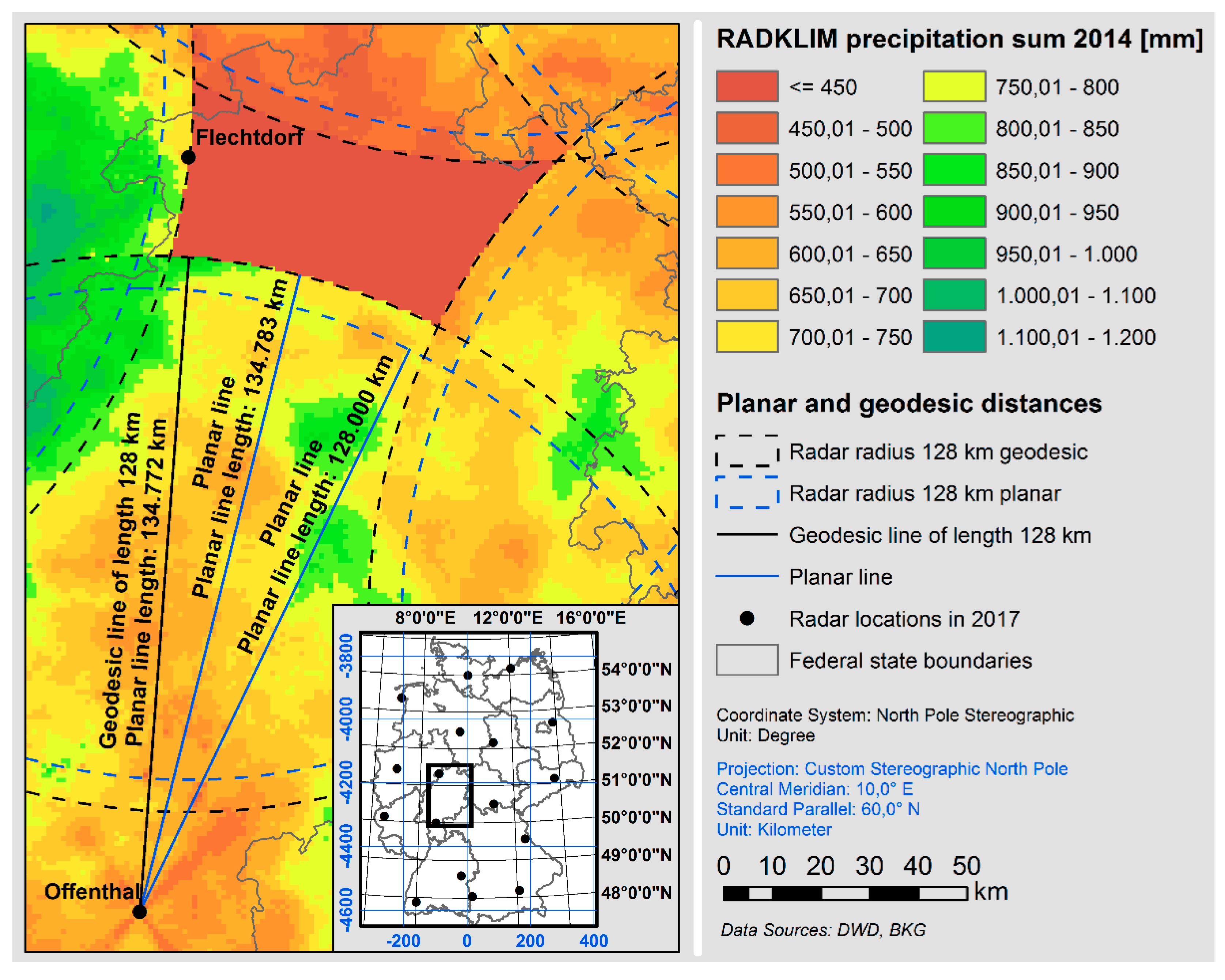
The distance to the nearest radar is split into four separate fields, which is due to changes in the radar network (new stations or altered locations) and the difference in the radar radius used for RADKLIM (128 km) and RADOLAN (150 km). As there were no changes to the radar hardware in the years 2010 and 2017, the radar stations for these two years were digitized from the coordinates given in [13] and the Euclidean distance of each pixel to the nearest radar within the given radius and year was calculated in the radar projection for RADKLIM and RADOLAN, respectively. However, the calculated maximum distances did not match the radar ranges that are visible in the precipitation composites since the calculated radius was too small. Consequently, the radius was extended in order to fill out the entire radar range and to obtain valid distance values for each pixel. As a result, the maximum distance values exceed the respective radius given by DWD by between 3.5 km in Northern Germany and up to 10 km in Southern Germany. This effect can be explained by the polar-stereographic radar projection’s increasing distortion of area towards the south and the differences between planar and geodesic distance calculations. Whereas the planar Euclidean distance corresponds to the length of a straight line on a plane surface, the geodesic line is the distance between two points on a curved surface, such as the Earth. Since the geodesic distance is greater and a projection to a planar surface tends to stretch surfaces in order to obtain a Cartesian grid, a geodesic line transformed into a planar projected coordinate system (such as the radar projection defined by DWD) is longer than a straight line drawn on a planar surface. The assumption, that the radar radius given by DWD is actually a geodesic distance and does not correspond to 128 or 150 km in their custom projected stereographic coordinate system could be confirmed by a comparison of planar and geodesic buffers around the radar locations with aggregated precipitation composites (see Figure 2). A geodesic buffer with a distance of 128 km around the radar locations is perfectly aligned with the radar ranges observed from the precipitation composites, but the maximum distance measured in the radar projection was 3.5 to 10 km higher. In contrast to this, a planar buffer of 128 km is too small and does not cover the actual radar range.
For the derivation of the three parameters related to wind energy plants (count, mean hub height and mean rotor diameter per radar pixel), the RADKLIM IDs were extracted to the wind energy point shapefile and summary statistics for each pixel were calculated. Subsequently, the statistics were exported to three separate rasters based on the RADKLIM ID raster.
Step 4: Creation of the output dataset
In order to prepare the concluding data collection step, the RADKLIM ID raster for Germany was converted to an ArcGIS file geodatabase point feature class containing the centroids of all 1 km2 RADKLIM grid cells. Subsequently, a list of all rasters which are supposed to be included in the dataset was created and their pixel values were extracted to the respective point features based on location.
The resulting dataset comprises 392,529 point features (rows in the attribute table) on a regular 1 km grid and the attribute table contains 67 fields (columns).

3.2. Rain Gauge Precipitation Dataset

3.2.1. Data Source and Accessibility

The rain gauge RR data in 1-minute resolution used for this dataset are freely available in the DWD Open Data Portal (https://opendata.dwd.de/climate_environment/CDC/observations_ germany/climate/1_minute/precipitation/). Measurement data are provided as zipped text files with one file per station and month and sorted in year folders. Downloading the dataset can be rather tedious as there is no option to automatically download an entire year folder although there are thousands of files per year which are not collected in any zip archives. The data files have an aperiodic structure, which means hours or days without precipitation are summarized in one line. Next to the precipitation data are zip archives with several metadata text files for each station containing information on measurement periods, devices, and time zones as well as station coordinates, height above sea level, and full station names. An additional metadata text file provides a summary of all gauges describing their coordinates, height, names and measurement periods.
For the analysis period 2006 to 2017, the precipitation was measured by tipping bucket or OTT Pluvio rain gauges at most of the stations and the data are provided in UTC time zone since the year 2000.

3.2.2. Data Processing, Aggregation and Validation

Step 1: Data availability check, data processing, and data cleaning
All precipitation data files for the period 2006 to 2017 were downloaded and unzipped into year folders using Python. Subsequently, all data were imported and converted into periodic monthly pandas DataFrames with one column per gauge and one row per minute. These DataFrames were then saved into the same uniform HDF5 file format as the radar data with one group per year and therein twelve monthly datasets. Internally, the data import and preprocessing is divided into several consecutive parts. First, data availability and completeness were checked and a dictionary with lists of files for import sorted by month was generated. For every year and station, the number of available month files was counted. If one or more month files were missing, the remaining files for this station were removed from the lists and all values for this station were set to pandas’ missing data value NaN throughout the entire year. This resulted in a loss of between 0.9 % of gauges in 2014 up to 20.8% in 2006 with an average loss of 4% (37 gauges) for the above period, but this data cleaning is necessary in order to reduce the bias of subsequent aggregated statistics due to incomplete time series and to obtain more reliable data for comparison. Next, each file was imported, and the three precipitation data columns representing weighing method (RS_01), dropper (RTH_01), and tipping bucket (RWH_01) measurement devices were merged and converted into a single-column DataFrame. Usually, only one data column contains valid values at a time, but in some cases, e.g., due to device changes or due to the use of ombrometers providing a combination of dropper and tipping bucket, there can be two columns with non-NaN values. With respect to the measurement accuracy and resolution, the value from the ‘RS_01’ column (weighing method), which was measured by Pluvio rain gauges in most cases, was selected where available. If it is NaN at the respective interval, the value from the ‘RTH_01’ (dropper) column was selected and if values in both of these columns are NaN, the value from the ‘RWH_01’ (tipping bucket) column was selected. Upon resampling, all gaps in the aperiodic data were filled with zeros since—assuming the data are correct—only rainless periods are summarized and NaN intervals are indicated by the value −999 in the original data. Finally, for each month, all single-column DataFrames were concatenated and the monthly DataFrames were saved to HDF5.
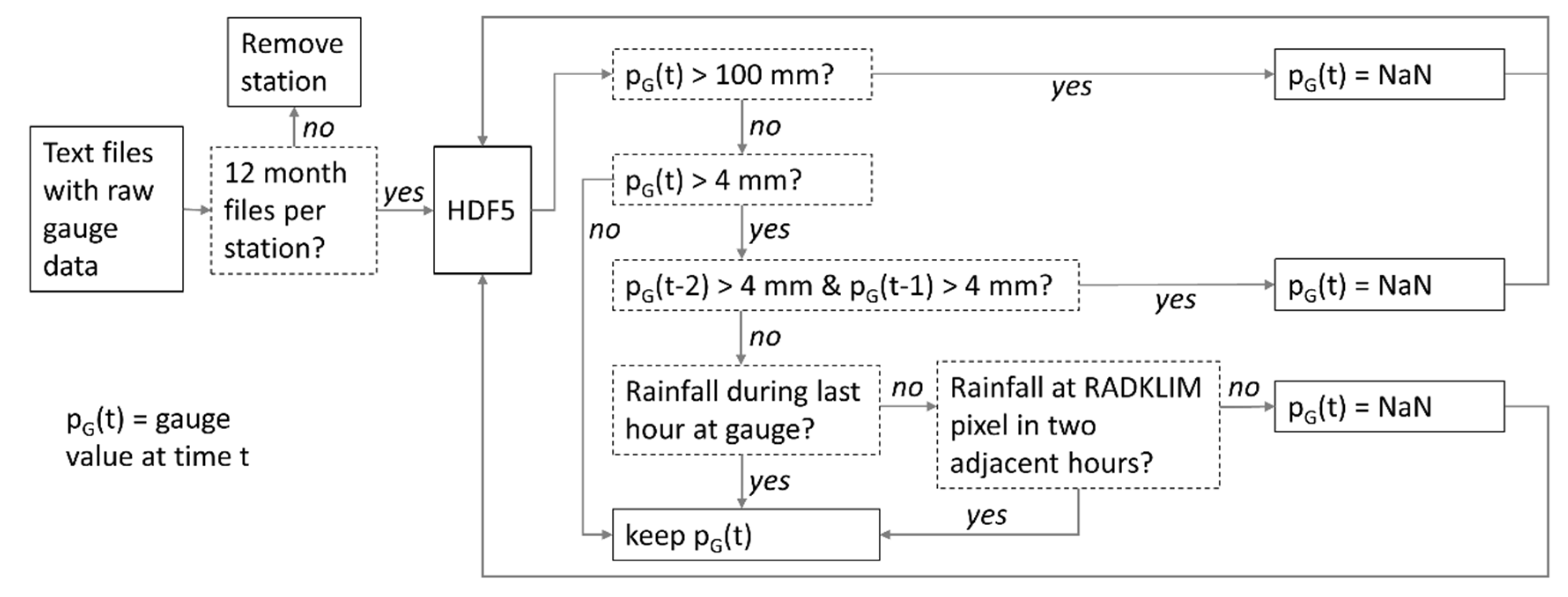
However, data validation showed that the raw gauge data contain a series of erroneous or at least questionable values, which could be summarized into three classes outlined below. Whereas comparable values were kept in the RADKLIM and RADOLAN data, they need to be corrected in the gauge dataset, which is regarded as ground-truth reference for the evaluation of the radar datasets. Consequently, an additional iterative data cleaning procedure has been applied to the HDF5 file containing the processed gauge data in order to account for each of these error types (see Figure 3):
  • Several extremely high minute values (121 min intervals between 312.44 and 487.56 mm at station 01669 in January 2008), which are regarded as impossible. Consequently, all intervals exceeding 100 mm were replaced by NaN in the HDF5 file without any further checks. The high threshold of 100 mm was chosen in order to ensure that no heavy rainfall events that may have been saved as aggregated value (e.g., a daily sum), e.g., due to hardware issues, are erased from the data without any further checks.
  • Very high values with missing entries or zeros in the raw data several minutes or hours beforehand (e.g., 57.27 mm at station 07104 at 06.06.2011 10:49 with previous entry 0.0 mm at 10:02; 55.17 mm at station 05158 at 30.09.2006 13:08 with previous entries all 0.0 mm). Such high values could be either erroneous data or also sum values for a previous time period during which a malfunction of the gauge occurred and the precipitation sum was added later. For such values, it is difficult to tell which of these cases holds true and how long the summarized period has been. However, as the gauge dataset needs to be reliable at least at an hourly temporal resolution for subsequent comparison to the radar data, a three-step validation was applied: First, all intervals exceeding 4 mm/min were regarded as potentially erroneous and identified from the HDF5 file. Second, for all exceeding intervals, the precipitation values of the gauge during the previous hour were checked. If there are any non-zero precipitation values, the gauge was assumed to have worked correctly and the value was kept. Third, if the gauge indicated no precipitation during the previous hour, the precipitation amount of the two adjacent hours of the corresponding RADKLIM pixel was consulted. If any of these indicated precipitation, the gauge value was kept. If both hours have a value of 0.0 mm at the RADKLIM pixel, the exceeding gauge value was set to NaN since it can either be considered as erroneous or the actual precipitation may have occurred at some unknown time in the past and the value is not representative for the point of time under review.
  • Sequences of several consecutive minutes with remarkably high values (e.g., at station 02532 on 15.06.2006, there are four consecutive entries with 10.75 mm/min between 8:01 and 8:04 AM). To address potential errors due to value repetitions in the data and their potentially significant effects on data aggregation results, the intervals exceeding 4 mm/min were additionally checked for the time between exceedances. If there are more than two consecutive intervals exceeding 4 mm/min, all intervals starting from the third were set to NaN.
The reasons for the observed errors and uncertainties are largely unknown and not indicated in the sparse gauge data documentation. It can be assumed, though, that several of the high outliers are actually sum values of longer time periods due to temporary malfunctions of the devices. Especially during heavy rainfall events measured by tipping bucket gauges, there may be design-inherent difficulties to continuously detect rain rates with high intensities. Errors related to missing NoData values (see Step 3 below), however, can most likely be attributed to data processing issues.
All in all, the number of gaps as well as unexpected and unexplainable errors in the raw gauge data is much higher than in the radar data, whereas the documentation of gauge data formats is much sparser and less comprehensive. Consequently, the gauge data processing necessitates a much higher effort for the handling of missing or erroneous data. Regarding the missing data, 435 out of 997 gauges in the final dataset have a largely complete time series without any hours regarded as NaN (field ‘G_nnan’, see Step 3 below). Moreover, for 598 gauges the number of NaN values is sufficiently low to have all annual precipitation sums for the entire period of 2006 to 2017 calculated. As for the radar data, all precipitation statistics calculated in the following are based on the generated HDF5 file.
Step 2: Creation of a point shapefile with gauge locations
Besides the precipitation data preprocessing, an ArcGIS file geodatabase point feature class with all gauge locations as well as metadata on beginning and end of the measurement period, station name, and number; height above sea level; and the federal state was generated from the metadata summary file. Since the gauge locations are provided as geographic coordinates, the spatial reference of this feature class is the Geographic Coordinate System WGS 84. Moreover, the RADKLIM and RADOLAN cell IDs corresponding to each station were extracted from the RADKLIM and RADOLAN ID rasters. The new ID fields added to the attribute table are the basis for the final merging of the gauge and radar datasets described in Section 3.3, since they provide the information in which RADKLIM or RADOLAN cell the respective gauges are located.
Step 3: Calculation of precipitation statistics
Most of the precipitation statistics calculated and the functions applied on the gauge dataset are identical to those for the radar datasets. But, in contrast to the calculations for the radar data, results are exported to the feature class attribute table directly from the DataFrames and without storage of intermediate files. The only major difference in the data exported to the feature classes pertains to the annual precipitation sums. In contrast to the radar dataset, the cleaned sums after the removal of low outliers, which is explained in Section 3.1.2, were exported for the gauge dataset. This is necessary due to erroneous values in the original gauge data. For gauge no. 01346, the data files contain the value 0.0 throughout the entire years 2006, 2007, and most of 2008 resulting in incorrect annual precipitation sums of 0 mm, 0 mm, and 32.29 mm, respectively. As this leads to heavily biased annual averages and because the gauge dataset values need to be regarded as a ground truth for subsequent data comparisons, these values must not be exported to the final dataset and were removed as outliers beforehand. Yet, a comparison of the cleaned and uncleaned annual sums showed that only one other gauge, no. 04501, which has an annual precipitation sum of 21.9 mm in the year 2006, is affected by comparable errors.
For the count of NaN values (field ‘G_nnan’), the different temporal resolutions of gauge (1 min) and radar datasets (60 min) had to be equalized in order to obtain comparable values. Hence, the gauge data were aggregated to hours whereby an hour was set to NaN if more than 10 out of 60 min intervals contain NaN values. Additionally, as stations with less than 12 monthly data files for one year are not contained in the HDF5 file for the respective year, the number of hours per missing year was added to the calculated NaN counts. Consequently, the total NaN count is the sum of NaN values actually contained in the HDF5 file plus the number of hours of each year removed by data cleaning procedures.
Step 4: Removal of gauge points with incomplete data collection
After the export of the annual precipitation sums, gauge points without precipitation data or without corresponding RADKLIM or RADOLAN cell ID—which can happen if they are close to the national border in an area not covered by radar—are deleted in order to keep only gauges with a complete dataset for comparison with the radar data.
The resulting rain gauge point shapefile comprises 997 point features (rain gauges) spread over Germany with a total of 37 fields in the attribute table.

3.3. Merging the Datasets

3.3.1. Methodology

In order to merge both precipitation datasets to the final rainfall data intercomparison dataset, both feature class attribute tables were joined to each other based on the RADKLIM ID. On the one hand, the gauge values were joined to the radar feature class by performing an outer join to keep all radar values. For radar pixels that contain a gauge, the respective gauge values were appended to the attribute table, whereas, for radar pixels without a gauge, the fields for gauge data contain NoData values (<Null>). On the other hand, the values of radar pixels containing a gauge were joined to the gauge feature class using an inner join that only keeps features with common RADKLIM IDs. Consequently, the gauge feature class is actually a subset of the radar feature class which contains only complete data collections for intercomparison as well as accurate gauge locations instead of radar grid cell centroids.
Finally, for publication, both feature classes were exported to shapefiles which can be read by all common GIS. However, shapefiles are not able to store the feature class-specific <Null> values (these are replaced by 0 upon export). Since in the radar feature class, <Null> values represent the status ‘no coverage’ (a pixel is either not covered by any radar or does not contain a gauge), which can be important for intercomparison, this information needs to be kept. Hence, to distinguish the actual value 0 from <Null> values, the latter were replaced by the value −99999 in both feature classes before export. Contrary to the radar shapefile, in the gauge shapefile, missing annual precipitation sums received the value 0 because the years are not necessarily uncovered but the data may have been removed due to incompleteness or erroneous data. Consequently, this shapefile contains −99999 only for parameters which could not be calculated such as the mean daily precipitation exceeding 20 mm if there is actually no such day.

3.3.2. Resulting Dataset

The final radar shapefile still comprises 392,529 point features (rows in the attribute table) on a regular 1 km grid, but after joining the gauge attribute fields, the attribute table now contains 98 fields (columns). The final gauge shapefile comprises 997 point features with exactly the same 98 fields as the radar shapefile in its attribute table.
All parameters that were calculated for two or all three rainfall datasets were prefixed with RK_ (RADKLIM), RO_ (RADOLAN), or G_ (Gauges) to identify the data origin. Thus, to compare, e.g., the mean precipitation sum in the hydrological winter half-year between all three precipitation datasets, the fields ‘RK_MWP’, ‘RO_MWP’, and ‘G_MWP’ need to be selected.

4. Data Use and Application

The rainfall data intercomparison dataset presented in this paper can be directly imported into all common GIS due to its shapefile format. It can be used for the creation of maps at any scale within Germany in order to, e.g.,
  • compare the rainfall datasets with each other and evaluate their quality,
  • identify the dataset best-suited for the respective study area and application,
  • improve the understanding of the inherent bias and error structure, especially of the two radar datasets, and to
  • provide precipitation maps and statistics as well as model inputs for the covered time period.
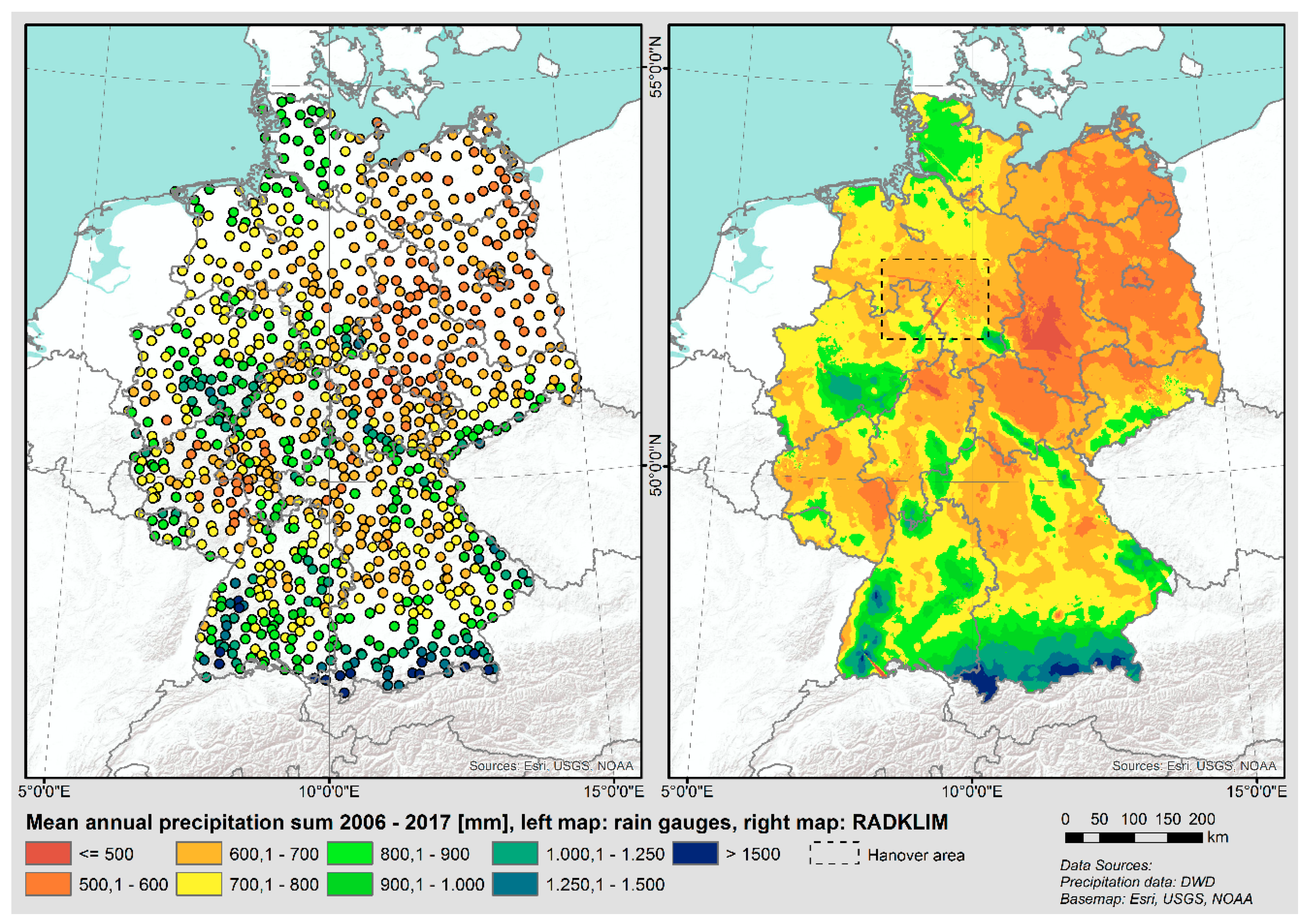
As an example for a straightforward comparison of the gauge and RADKLIM datasets, Figure 4 shows the cleaned mean annual precipitation sums of the gauges (gauge shapefile, field ‘G_MAPc_l’) as well as the RADKLIM mean annual precipitation sums (radar shapefile, field ‘RK_MAP’).
Besides the precipitation averages, the rain gauge data-based map (Figure 4 on the left) also shows the nationwide spatial distribution of gauge stations in the gauge shapefile, whereas the RADKLIM map (Figure 4 on the right) shows the clipped 1 km2 grid of the radar shapefile. The comparison of both maps shows a mainly consistent spatial precipitation distribution in the gauge and RADKLIM datasets with mountain ranges being distinguishable and a decrease of precipitation amounts from west to east, which is characteristic for the transition from a maritime to a more continental climate in Germany. However, the maps also indicate slightly higher gauge values in some regions and the RADKLIM map shows several spatial structures that can be attributed to radar artifacts. As an example, there is a series of striking clusters of pixels with outstandingly low and high values around the radar station in Hanover, Lower Saxony, as well as two lines of pixels with remarkably low values running from the radar station in western and southwestern directions. The former are insufficiently corrected or overcorrected (‘Reverse Speckle’) false echoes, which are a common problem due to the low radar beam height at close range from the radar, whereas the latter are so-called spokes, which can occur if the radar beam is blocked close to the radar or if an azimuth angle is not scanned at all [10].
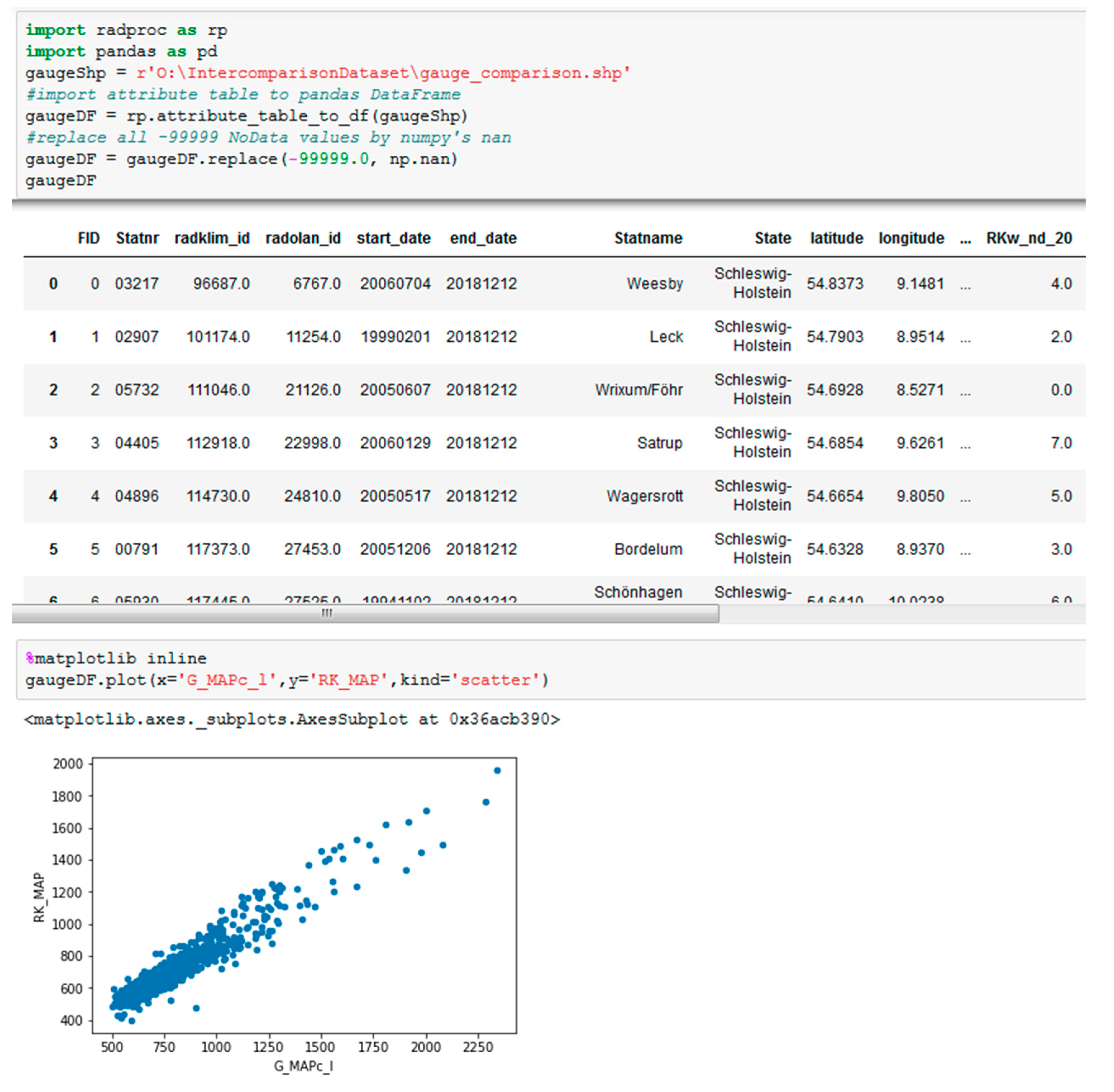
Beyond the applications presented above, the rainfall data intercomparison dataset can also be used for statistical analyses. Examples include the calculation of differences and ratios between precipitation datasets, exploratory data analysis, plotting or the fitting of regression models in order to analyze the correlations and dependencies between the RADKLIM and RADOLAN data and other parameters such as the height above sea level or the distance to the next radar. A straightforward way for users of ArcGIS to import the intercomparison dataset into the Python ecosystem, which provides rich functionality for statistical analyses, is shown in Figure 5. It shows the import of the gauge shapefile attribute table into a DataFrame in Python using the radproc package in a Jupyter Notebook [28] and how to plot selected data columns against each other as a scatter plot. This quick analysis confirms the assumption derived from the map comparison (see Figure 4) that gauge and RADKLIM values match quite well in general, but the gauge values tend to be higher than the RADKLIM values.

Author Contributions

Conceptualization, J.K. and G.K.; methodology, J.K.; software, J.K.; validation, J.K. and G.K.; formal analysis, J.K.; data curation, J.K.; writing—original draft preparation, J.K.; writing—review and editing, B.T., G.K., B.B., and J.K.; visualization, J.K.; supervision, G.K., B.B., and B.T.

Funding

This research received no external funding.

Acknowledgments

The authors are grateful to DWD for providing open access radar and rain gauge data and thank Angie Faust for proofreading.

Conflicts of Interest

The authors declare no conflicts of interest.

References

  1. Thorndahl, S.; Einfalt, T.; Willems, P.; Nielsen, J.E.; Veldhuis, M.C.T.; Arnbjerg-Nielsen, K.; Rasmussen, M.R.; Molnar, P. Weather radar rainfall data in urban hydrology. Hydrol. Earth Syst. Sci. 2017, 21, 1359–1380. [Google Scholar] [CrossRef] [Green Version]
  2. Krajewski, W.F.; Kruger, A.; Smith, J.A.; Lawrence, R.; Gunyon, C.; Goska, R.; Seo, B.C.; Domaszczynski, P.; Baeck, M.L.; Ramamurthy, M.K.; et al. Towards better utilization of NEXRAD data in hydrology: An overview of Hydro-NEXRAD. J. Hydroinformatics 2011, 13, 255–266. [Google Scholar] [CrossRef]
  3. Seo, B.C.; Krajewski, W.F.; Kruger, A.; Domaszczynski, P.; Smith, J.A.; Steiner, M. Radar-rainfall estimation algorithms of Hydro-NEXRAD. J. Hydroinformatics 2011, 13, 277. [Google Scholar] [CrossRef]
  4. Leijnse, H.; Uijlenhoet, R.; Hazenberg, P. Radar rainfall estimation of stratiform winter precipitation in the Belgian Ardennes. Water Resour. Res. 2011, 47, 257. [Google Scholar]
  5. Gjertsen, U.; Salek, M.; Michelson, D.B. Gauge-adjustment of radar-based precipitation estimates–a review. Cartogr. Perspect. 2003, 1. [Google Scholar] [CrossRef]
  6. Goudenhoofdt, E.; Delobbe, L. Evaluation of radar-gauge merging methods for quantitative precipitation estimates. Hydrol. Earth Syst. Sci. 2009, 13, 195–203. [Google Scholar] [CrossRef] [Green Version]
  7. Berne, A.; Krajewski, W.F. Radar for hydrology: Unfulfilled promise or unrecognized potential? Adv. Water Resour. 2013, 51, 357–366. [Google Scholar] [CrossRef]
  8. MeteoSolutions GmbH. Projekt RADOLAN–Routineverfahren zur Online-Aneichung der Radarniederschlagsdaten mit Hilfe von Automatischen Bodenniederschlagsstationen (Ombrometer). Zusammenfassender Abschlussbericht für die Projektlaufzeit von 1997 bis 2004. Available online: https://www.dwd.de/DE/leistungen/radolan/radolan_info/abschlussbericht_pdf.pdf?__blob=publication File&v=2 (accessed on 19 April 2018).
  9. Winterrath, T.; Rosenow, W.; Weigl, E. On the DWD Quantitative Precipitation Analysis and Nowcasting System for Real-Time Application in German Flood Risk Management. IAHS Publ. 2012, 351, 323–329. [Google Scholar]
  10. Erstellung Einer Radargestützten Niederschlagsklimatologie; Berichte des Deutschen Wetterdienstes No. 251. 2017. Available online: https://www.dwd.de/DE/leistungen/pbfb_verlag_berichte/pdf_einzelbaende/ 251_pdf.pdf?__blob=publicationFile&v=2. (accessed on 29 March 2019).
  11. RADKLIM Version 2017.002: Reprocessed Gauge-Adjusted Radar Data, One-Hour Precipitation Sums (RW). Available online: https://opendata.dwd.de/climate_environment/CDC/grids_germany/hourly/ radolan/reproc/2017_002/bin (accessed on 25 June 2019).
  12. RADKLIM Version 2017.002: Reprocessed Quasi Gauge-Adjusted Radar Data, 5-Minute Precipitation Sums (YW). Available online: https://opendata.dwd.de/climate_environment/CDC/grids_germany/ 5_minutes/radolan/reproc/2017_002/bin/ (accessed on 25 June 2019).
  13. Deutscher Wetterdienst. RADKLIM: Beschreibung des Kompositformats und der Verschiedenen Reprozessierungsläufe. Version 1.0. 2018. Available online: https://www.dwd.de/DE/leistungen/ radarklimatologie/radklim_kompositformat_1_0.pdf;jsessionid=0889B3A8CB74341FAA652DB2A4FB7F63.live11041?__blob=publicationFile&v=1 (accessed on 26 March 2019).
  14. A Rainfall Data Inter-Comparison Dataset for Germany: Version 1.0. Available online: https://zenodo.org/ record/3262172 (accessed on 29 June 2019).
  15. Deutscher Wetterdienst. RADOLAN und RADVOR: Beschreibung des Kompositformats. Version 2.4.4. 2018. Available online: https://www.dwd.de/DE/leistungen/radolan/radolan_info/radolan_radvor_op_ komposit_format_pdf.pdf?__blob=publicationFile&v=11 (accessed on 26 March 2019).
  16. Eichhorn, M.; Scheftelowitz, M.; Reichmuth, M.; Lorenz, C.; Louca, K.; Schiffler, A.; Keuneke, R.; Bauschmann, M.; Ponitka, J.; Manske, D.; et al. Spatial Distribution of Wind Turbines, Photovoltaic Field Systems, Bioenergy, and River Hydro Power Plants in Germany. Data 2019, 4, 29. [Google Scholar] [CrossRef]
  17. Radproc–A Gis-Compatible Python-Package for Automated Radolan Composite Processing and Analysis; Zenodo. 2018. Available online: https://zenodo.org/record/2539441 (accessed on 25 June 2019).
  18. Mckinney, W. pandas: A Foundational Python Library for Data Analysis and Statistics. Available online: https://www.dlr.de/sc/Portaldata/15/Resources/dokumente/pyhpc2011/submissions/pyhpc2011_submission_9.pdf (accessed on 31 July 2019).
  19. Hierarchical Data Format. Available online: https://portal.hdfgroup.org (accessed on 18 December 2018).
  20. Kreklow, J. Facilitating radar precipitation data processing, assessment and analysis: A GIS-compatible python approach. J. Hydroinformatics 2019, 21, 652–670. [Google Scholar] [CrossRef]
  21. Oliphant, T.E. A Guide to NumPy; CreateSpace: Scotts Valley, CA, USA, 2006. [Google Scholar]
  22. Stephan, K. Erfahrungsbericht zur Verwendung des PULL-Kompositverfahrens zur Erstellung des Radolan-Komposits (RZ-Komposit). DWD Interner Ber. 2007, in press. [Google Scholar]
  23. RADOLAN-Information Nr. 17. Available online: https://www.dwd.de/DE/leistungen/radolan/ radolan_info/radolan_info_nr_17.pdf?__blob=publicationFile&v=3 (accessed on 17 June 2019).
  24. Weigl, E.; Winterrath, T. Radargestützte Niederschlagsanalyse und –vorhersage (RADOLAN, RADVOR-OP). Promet 2009, 35, 78–86. [Google Scholar]
  25. Tukey, J. Exploratory Data Analysis; Addison-Wesley: Reading, MA, USA, 1977. [Google Scholar]
  26. Germann, U.; Galli, G.; Boscacci, M.; Bolliger, M. Radar precipitation measurement in a mountainous region. Q. J. R. Meteorol. Soc. 2006, 132, 1669–1692. [Google Scholar] [CrossRef]
  27. Meischner, P. Weather Radar: Principles and Advanced Applications, 1st ed.; Springer: Berlin/Heidelberg, Germany, 2004. [Google Scholar]
  28. Project Jupyter. Jupyter Notebook, 2014–2019. Available online: https://jupyter.org/ (accessed on 17 June 2019).
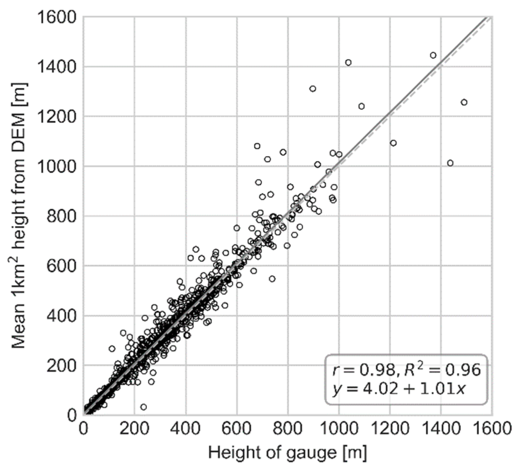
Figure 1. Comparison of height above sea level derived from the gauge metadata (field ‘G_height’) and from the Shuttle Radar Topography Mission (SRTM) Digital Elevation Model (DEM) aggregated to 1 km2 (‘height_dem’) for the 997 points in the gauge shapefile.
Data 04 00118 g001
Figure 2. Differences between planar and geodesic distance calculation in the projected, Cartesian stereographic coordinate system defined for the radar products by Deutscher Wetterdienst (DWD). The very low precipitation values in the northern area, which are due to several months of missing data during the upgrade of the radar Flechtdorf in 2014, provide an ideal radar range for the distance validation.
Data 04 00118 g002
Figure 3. Schematic rain gauge data cleaning workflow.
Data 04 00118 g003
Figure 4. Mean annual precipitation sum 2006–2017 calculated from rain gauges (map on the left) and RADKLIM (map on the right). The dashed rectangle in the RADKLIM map indicates the area around the radar station in Hanover discussed in the text.
Data 04 00118 g004
Figure 5. Importing the gauge shapefile into a DataFrame and plotting the mean annual precipitation sums of gauges and RADKLIM against each other.
Data 04 00118 g005
Table 1. Overview and description of the most important attribute fields contained in the rainfall data intercomparison dataset. All fields marked with * were calculated for all three precipitation datasets, fields marked with ** were calculated only for the two radar datasets. These fields are prefixed with “RK_” (derived from the hourly RADKLIM RW product), “RO_” (RADOLAN RW) or “G_” (rain gauge data) in the attribute table.
Field NameParameter DescriptionUnit
*MAPMean annual precipitation sum 2006–2017mm
**MAPcMean annual precipitation sum cleaned from extreme outliersmm
*MAPc_lMean annual precipitation sum cleaned from extreme lower outliersmm
*MSPMean summer precipitation sum (May–October)mm
*MWPMean winter precipitation sum (November–April)mm
*2006, …, *2017Precipitation sum of the year 2006, 2007, …, 2017mm
*nnanTotal number of NoData entries in the period 2006–2017-
*s_nd_1Number of days exceeding a precipitation sum of 1 mm in the summer-
*s_MDP_1Mean precipitation of all days exceeding a precipitation sum of 1 mm in the summermm
*s_nd_20Number of days exceeding a precipitation sum of 20 mm in the summer-
*s_MDP_20Mean precipitation of all days exceeding a precipitation sum of 20 mm in the summermm
*w_nd_1Number of days exceeding a precipitation sum of 1 mm in the winter-
*w_MDP_1Mean precipitation of all days exceeding a precipitation sum of 1 mm in the wintermm
*w_nd_20Number of days exceeding a precipitation sum of 20 mm in the winter-
*w_MDP_20Mean precipitation of all days exceeding a precipitation sum of 20 mm in the wintermm
height_demAverage height above sea level per radar pixelm
nwepNumber of wind energy plants in the respective radar pixel-
wep_heightAverage hub height of all wind energy plants per pixelm
wep_diaAverage rotor diameter of all wind energy plants per pixelm
**dist10Distance to closest radar station in the year 2010km
**dist17Distance to closest radar station in the year 2017km