1. Introduction
Autonomous navigation is crucial for search, rescue and remote inspection because teleoperation by video stream is extremely challenging when moving close to buildings or trees and in an indoor environment. Besides, the Global Positioning System (GPS) may not be reliable in cases of low satellite coverage and signal multipath interference [
1,
2]. Using a compact laser scanner can offer an alternative solution. However, such a solution is expensive and the laser has low frequency [
3]. The vision-based solution seems particularly suitable to the autonomous navigation in terms of the weight, cost and information it can provide. With an onboard camera, the drone can both estimate the ego-motion and obtain the information on the environment simultaneously.
Visual geometric methods such as direct, semi-direct and feature-based visual odometry are well known [
4,
5]. However, geometric methods lack robustness for a number of very common effects, such as illumination changes, movement of dynamic objects, different camera calibrations, low-textured environments, noise and motion blur. Data-driven visual odometry using deep learning methods and low-cost cameras is the most promising approach.
Deep data-driven visual odometry has the potential for high learning capability and robustness of camera parameters and challenging environments [
5,
6]. However, deep models typically require large computational resources for training and inference mode. Besides that, deep models need large labelled datasets for successful training. Complexity reduction of the model can be achieved by narrowing the scope of application to a particular domain of use. However, even a tiny deep model requires significant computational resources and a large labelled training set, which leads to a significant overhead and slow adaptation to the new condition and environment.
The conventional convolutional neural network, comprised of a convolutional filter-based multilayer feature extractor and fully connected neural layers forming the decision rules, is an a very popular model choice for the analysis of image data [
7,
8]. This being said, conventional convolutional neural networks have a number of disadvantages, such as their inability to analyze the processes occurring in time, and high computational complexity of the learning algorithm based on backpropagation [
9]. In addition, making an advance estimate of the required number of neurons in each convolutional layer is complicated. In contrast, a neural network training approach with unsupervised learning methods based on growing neural gas and their modifications offers better prospects [
1,
10]. Moreover, the convolutional feature extractor combined with sparse coding is characterized by its ability to operate on small datasets or significant target data imbalance in an unlabelled dataset, which can be dealt with by the fine-tuning of feature extractor using a criterion based on efficiency of decision rules [
8]. End-to-end fine-tuning in hybrid models is often limited by many inconsistencies. In this case, fine-tuning can be effectively performed by any trajectory-based metaheuristic search algorithm. However, the training process speed depends on computation complexity of model.
The ego-motion estimation task is the most important part of visual navigation process and it can be formulated as a regression analysis for position displacement prediction. The support vector machine and extreme learning machine (ELM) are widely used as regression models in hybrid intelligent systems, especially with constraints on availability of computational resources and the size of labelled dataset. In this case, ELM is characterized by the most rapid training to obtain the least-squares solution of regression problem [
11]. In order to eliminate overfitting, which occurs when the number of hidden layer nodes is large, it is relevant to investigate the incremental learning via successive addition of hidden nodes.
The information-extreme classifier of a high-level feature representation is one of the most promising approaches to implementing trainable obstacle avoidance capabilities in terms of computation efficiency and generalizing abilities. The main idea of information-extreme techniques is to transform input space of primary features into binary Hamming space with radial basis decision rules. This approach provides high computational efficiency because simple operation of comparison with thresholds and Hamming distance calculation based on logical XOR operation and non-zero bit counting are used. However, fast threshold optimization methods for feature encoding have not yet been proposed. In this case, feature inductions based on decision tree and boosting are two particularly promising algorithms which can speed up threshold optimization for binary feature encoding [
12,
13].
In order to implement autonomous navigation and identification of obstacles under the conditions of constrained computational resources and limited labelled training set, this paper proposes a multilayer convolutional sparse coding model for feature extraction from spatial-temporal visual data. In addition, the training algorithms based on unsupervised pretraining and supervised fine-tuning of feature extractor to maximize supervised learning efficiency of information-extreme classifier and extreme-learning regression model are also proposed.
2. Data Description and Data Model Design
To prepare the input mathematical description of the intelligent information system, KITTI VO/SLAM benchmarks 07 and 09 from Kaggle were used. The datasets contain the image frame sequence captured by the moving video camera and the corresponding tri-axis ground truth movement data reported by GPS and LiDaR (dataset:
http://www.cvlibs.net/datasets/kitti/raw_data.php?type=residential,
https://vision.in.tum.de/data/datasets/visual-inertial-dataset; dataset license: Creative Commons Attribution-NonCommercial-ShareAlike 3.0 License, Creative Commons Attribution-NonCommercial-ShareAlike 3.0 License, Creative Commons 4.0 Attribution License CC BY 4.0) [
8]. Since this dataset was recorded at a relatively low frame rate (10 frame per second) by driving in urban areas many dynamic objects and the speed of the driving was up to 90 km/h, some image pre-processing was necessary. This was achieved by applying the resizing, gray scaling and un-distorting functions from an open-source robotic operation system [
9]. Whilst it required the camera calibration parameters, high accuracy was not needed. The training and test video sequences from the KITTI Vision dataset were used. The images were downscaled to 200 × 200 due to memory and computation resource limitations.
The main adopted methodological principles of data analysis model design are as follows:
- -
using more than 2 subsequent frames to determine the movement between the two last frames, which allows for better context detection and increase of the decision accuracy;
- -
hierarchical feature representation, which allows describing complex features with a smaller number of parameters;
- -
avoidance of subsampling for preservation of larger quantity of information (data shifts, deformation and scale), which is important for regression analysis of camera movement in time and space, especially in absence of end-to-end learning;
- -
low-computational-complexity decisions rules, which reduce the time needed for efficiency evaluation and feature extractor tuning.
The trainable model of the visual navigation should provide obstacle avoidance and control of UAV’s (unmanned aerial vehicle) own position through odometry. The proposed model of visual navigation can be trained as an independent system or as an auxiliary parallel error corrector for geometric methods of visual odometry. In case of auxiliary option, both models must be synchronized.
Figure 1 depicts the schematic of the navigational system for a compact drone. A convolutional neural network which takes inputs in a form of a multichannel image formed by a series sampling of successive video frames in grayscale format is used to extract the feature representation of visual observations. A multilayered structure of Convolutional Neural Network (CNN) is used to form a high-level feature representation. Convolutional filters in the proposed CNN are subjected to unsupervised training layer by layer. An information-extreme classifier is then trained in supervised mode on the samples encoded by the corresponding high-level features. This classifier is then used to predict obstacles and for output of the corresponding response. The ELM-based regression model uses the visual features to predict the relative position change between two consecutive frames. From five consecutive observations, this component predicts position displacement along the x-axis and y-axis, and orientation (yaw) of the second frame with respect to the first frame.
The 4-layer architecture of the convolutional neural network is shown in
Figure 2. The first layer of the CNN contains standard convolutional filters with different kernels: 5 × 5, 3 × 3 and 1 × 1. The parameter
regulates the number of filters. To keep the size of feature maps formed by multiple-scale filters unchanged, the technique of padding by zeros is used [
8]. Corresponding stride parameters of scanning a feature map with multiple-scale filters for the second and third layers are 3 and 2, respectively. The Orthogonal Matching Pursuit (OMP) algorithm and rectifier function,
, are used for calculating each multi-channel pixel of feature map [
10]. To prevent information loss, the feature map can be doubled using the function
.
To train the regression model
represented by the single-hidden-layer feedforward network (SHFN), output variable
which corresponds to position displacement in terms of translation vector
and rotation vector
of the camera
, a set of
training data consisting of visual features, is used, where
. The SHFN with
R additive hidden nodes and activation function
(x) can be represented by:
where
is the weight vector linking the input layer with the
rth hidden node,
is the threshold of the
rth hidden node,
is the weight vector linking the output layer with the
rth hidden node,
is the output of the network with respect to the input vector
, and
is the activation function that can be any bounded non-constant piecewise continuous functions.
The network with
R hidden nodes can approximate these
N samples with zero error when all the parameters are allowed to be adjusted freely, i.e., there exist
,
and
. The above
equations can be compactly rewritten as the matrix equation
, where
Here,
H is called the hidden layer output matrix of the SHFN.
The information-extreme classifier under inference mode makes decision on belonging of input datapoint
with appropriate binary representation
to one class of turn from set
, according to the maximum value of membership function
through the expression
In this case, membership function
, the optimal container of which has support vector
and radius
is derived from:
Binary encoding of datapoint is carried out by concatenation of decision paths from ensemble of trees , ... , . Datapoint is classified in the leaf node by trees. Each decision node receives a unique identifier. If a test is satisfied in a node, then the corresponding bit is asserted. Finally, the encodings for each tree are combined by concatenation (or more generally by hashing the features ID onto a smaller-dimensional space) [143,134].
3. Training Algorithm Design
The main adopted methodological principles of machine learning algorithm design are as follows:
- -
uniting the competitive learning principles with sparse coding to reduce the training data sample size requirements and improved convergence during the feature extractor pretraining;
- -
training decision rules on the basis of fast randomized least-squares solvers (Gram–Schmidt process, and Moore–Penrose pseudoinverse) or decision trees-inspired techniques (random forest, random subspace, and adaptive boosting);
- -
metaheuristic optimization for harmonization of hybrid data analysis model components and improved convergence to the global model efficiency criterion optimum;
- -
complex criterion of the model efficiency is formed as a multiplicative aggregation of partial efficiency criteria aimed at the optimal feature extractor configuration which simultaneously improves all partial criteria.
The aim of the machine learning process of the navigation system is to determine the optimal vector of parameter
, which maximize the complex criterion as follow:
where
—learning effectiveness of recognition of obstacle averaged by the set of classes learning criterion;
—regression mean square error for the change of camera coordinates in space;
—computational complexity criterion of feature extraction algorithms;
,
, and
—the maximum possible value of the classifier training efficiency informational criterion, the minimum allowable values of regression model error and computational complexity of the system’s algorithms criterion, respectively; G—admissible domain of parameters affecting feature extraction and decision-making.
It is proposed to carry out unsupervised training of feature extractor using the growing sparse coding neural gas technique, based on the principles of growing neural gas and sparse coding. In this case, the dataset for training convolutional filters is formed by cropping the 3-dimensional patches of input images or feature maps. The shape of each patch is equivalent to corresponding filter shape. These patches reshape to 1-dimensional vectors, arriving at the input of the algorithm of growing sparse coding neural gas, and the basic stages of which are given below:
the counter of learning vectors t is initialized to be 0;
two initial nodes (neurons) and are assigned by random choice out of the training dataset. Nodes and are connected by the edge, the age of which is zero. These nodes are considered non-fixed;
the following vector x, set to the unit length (L2-normalization), is selected;
each basis vector is set to the unit length (L2-normalization);
the measure of similarity of input vector
x to basis vectors
is calculated for sorting
where
is the nearest node and
is the second nearest node by proximity node;
the age of all incidents is increased by unity;
if is fixed, go to step 9, otherwise, go to step 10;
if go to step 12. Otherwise, a new non-fixed neuron is added to the point which coincides with the input vector ; besides, a new edge that connects and is added, and then go to step 13;
node
and its topological neighbors (the nodes connected with it by the edge) are displaced in the direction to input vector
x according to the Oja’s rule [
13] by:
where
, and
are the vector of correction of weight coefficients of the neuron-winner and its topological neighbors, respectively;
and
are the constants of the updated force of weight coefficients of the neuron-winner and its topological neighbors, respectively
; ,
, and
are the initial, current and final value of learning rate, respectively;
if the neuron is labelled as fixed;
if and are connected by the edge, its age is nulled, otherwise, a new edge with the zero age is formed between and ;
all edges in the graph with the age of more than are removed. In the case when some nodes do not have any incident edges (become isolated), these nodes are also removed;
if , proceed to step 15, otherwise, increment the step counter t by 1 described as and proceed to step 3;
if all neurons are fixed, the algorithm implementation stops, otherwise, proceed to step 3 and a new learning epoch begins (repetition of the training dataset).
The information-extreme classifier that evaluates belonging of jth datapoint with features to one of the Z classes performs feature encoding using boosted trees and decision rules constructed in radial basis of binary Hamming space. In this case, there is the training set, , where is the size of dataset and is the label of jth pixel, which correspond to one class from set of classes . The training of boosted information-extreme classifier is performed according to the following steps:
Initialize weight .
Initialize step counter = 1.
Bootstrap from using probability distribution .
Train decision tree on using entropy criterion to measure the quality of split.
Perform binary encoding of datapoint
from
using concatenation of results from
trees. In this case, each decision tree produces a binary code where each non-zero bit corresponds to a node of decision path from root to leaf node [
12,
14]. The output of this step is a binary matrix
, where
is the number of induced binary features and
is the number of samples corresponding to class
. Hence, the equality
condition is met.
Build information-extreme decision rules in radial basis of binary Hamming space and compute optimal information criterion:
where
is a set of concentric radiuses with center
(support vector) of data distribution in class
, which is computed using the rule:
where
—training efficiency criterion of decision rule for class
, which is computed as the normed modification of the Kullback’s information measure [
13]:
where
, and
are the false-positive and false-negative rates of classification of input vectors as belonging to the class
;
ς is any small non-negative number, introduced to avoid uncertainty when being divided by zero.
A conventional way to increase the learning efficiency is a reduction of the multi-class classification problem to the series of the two-class one by the principle “one-against-all”. In this case, to avoid the problems of class imbalance, due to the majority of negative datapoints in datasets, a synthetic class is an alternative to class . The synthetic class is represented by datapoints of the remaining classes, which are the closest to support vector , where is the volume of the training dataset of class .
Test obtained information-extreme rules on dataset and compute the error rate for each sample from . Under the inference mode, decision on belonging of datapoint to one class from set is made according to the maximum value of membership function through the expression In this case, membership function of binary representation b of input datapoint x to class , the optimal container of which has support vector and radius is derived from Equation (5).
Update proportional to errors on datapoint .
If , abort the loop.
k = k + 1.
If , where K is the maximum number of trees, go to step 2.
Orthogonal incremental ELM is proposed to be used as a regression model. It avoids redundant nodes and obtains the least-squares solution of equation
by incorporating the Gram–Schmidt orthogonalization method into well-known incremental ELM. rigorous proofs in theory of convergence of orthogonal incremental extreme learning are given by Ying [
11]. The training of orthogonal incremental ELM is performed according to the following steps:
Set the maximum number of iterations and expected learning accuracy .
For = 1,…, do
Increase by one the number of hidden nodes: .
Randomly generate one hidden node and calculate its output vector .
If
r = 1 then
else
If
calculate the output weight for the new hidden node:
and calculate the new residual error:
else
.
If , abort the loop.
In order to approximate the global optimum of complex criterion during training of decision rules and feature exctactor fine-tuning, the use of simulated annealing metaheuristic algorithm is proposed [
13]. The efficiency of the simulated annealing algorithm depends on the implementation of the
create_neighbor_solution procedure, forming a new solution
si on the
ith iteration of the algorithm.
Figure 3 shows a pseudocode of the simulated annealing algorithm, which is implemented by the
epochs_max iterations, each of which function
f is calculated by passing a labelled training dataset through the model of the system of detection and calculation of a complex criterion (6).
An analysis of the pseudocode in
Figure 3 shows that current solution
, in relation to which new best solutions
are sought for, is updated in case of providing a new solution of the criterion increase (1), or randomly from the Gibbs distribution [
13]. In this case, an initial search point that is formed by the
create_initial_solution procedure can be either randomly generated or a result of the preliminarily training by another algorithm. To generate new solutions in the
create_neighbor_solution procedure, it is proposed to use the simplest non-adaptive algorithm, which can be represented as:
where
uniform_random is the function of generation of a random number from the uniformed distribution from the assigned range;
step_size is the size of a range of the search for new solutions, neighboring to
.
4. General Implementation and Setup Remarks
Autonomous navigation implementation is foreseen on 1 or 2 Raspbery Pi 3+ single-board 64-bit computers. They are equipped with CPU Broadcom BCM2837B0, Cortex-A53 (ARMv8) 64-bit SoC @ 1.4GHz and have 1GB of RAM. The official Raspbian operating system is 32-bit only and various other 64-bit have numerous problems with input–output device drivers, and hence, Debian Stretch is compiled for 64-bit SoC Broadcom BCM2837 Cortex-53 chip.
Training and inference regimes were implemented using Opencv 3.4, Tensorflow HRT with contributed modules and Robot Operating System Melodic Morenia (for arm64) with ORB-SLAM libraries. The libraries were optimised using single instruction, multiple data (SIMD) technologies (NEON-instruction). Jemalloc was installed to manage a given memory space. Image preprocessing was done with Opencv. Orthogonal Matching Pursuit, decision trees, ELM and growing sparse coding neural gas were implemented on Tensorflow framework for both training and inference.
For the purposes of testing the error corrector regime, dataset pre-processing and subsequent processing based on geometric odometry ORB-SLAM with a constraint on the maximum keypoint number limited to 100 was performed. The results were saved in a text file. After this, the proposed model was trained on a half of the KITTI dataset sequence. It is worth mentioning that for classifier training purposes, manually labelled turn samples taken from various sequences of KITTI dataset were used. A classifier in this case plays a regularizing role. The last step is the model launched in the inference mode to generate the final result taking into account ORB-SLAM results.
5. Simulation Results and Discussion
Parameters
and
values affect both the informative nature of the feature representation and the degree of computational complexity. For the purposes of this paper, computational complexity is measured by the quantity of “Mul” and “Add” operations performed at the time of convolutional operations with an image or a feature map. The computational complexity for the network architecture in
Figure 2 can be calculated as:
The optimal configuration of the convolutional extractor or the classifier and the regression model may differ, as they are responsible for different tasks. A complex criterion (6) offers an acceptable compromise between accuracy of the decision rules and the computational complexity of the visual feature extractor.
The set of recognition classes describes the characteristic obstacles and the corresponding response commands, and has a power . The first class of recognition characterizes the forward movement without turning. Classes and correspond to the left turn of 45 and 90 degrees, respectively. Classes and correspond to the right turn of 45 and 90 degrees, respectively. The size of the corresponding training and test sets for each class is . The regression model was trained on a half of the total length of the KITTI dataset sequence. KITTI-0.7 and KITTI-0.9 were used. The length of KITTI-0.7 sequence is equal to 1100 and the length of KITTI-0.9 sequence is equal to 1590.
It is proposed first to train the model using the unsupervised pretrained feature extractor via growing sparse coding neural gas without fine-tuning. In this case, three fixed values of the training dataset reconstruction parameter ν were used during training. This parameter directly affects the number of feature map channel .
In order to improve the results of machine learning of the visual navigation system, informativeness of feature description was increased by fine-tuning of the unsupervised trained convolutional filters parameters, which are depicted in
Figure 2. In this case, the following parameters of simulated annealing algorithm were used:
= 0.98,
= 10,
epochs_max = 3000, and
step_size = 0.001. Each fine-tuning step involved a re-training of a regression model and classifier. A simulation was performed for the three fixed values of parameters
and
(
Table 1) to evaluate the tendency of change in average values of the partial and complex criteria during the growth of such parameters affect the size of the feature extractor (
Figure 2). The optimal parameter values were determined for the KITTI-07 open dataset.
The analysis of
Table 1 shows that increases in parameter values
and
tend to increase both the reliability and computational complexity (20) of the decision rules of the classifier and the regression model. At the same time, the increase in parameter
has a negligible effect on the overall classifier efficiency due to the corresponding decrease in the learning efficiency with a substantial growth of the feature space, while the regression error is equally sensitive to the values of parameters
and
.
However, considering that, as and grow, the reliability of decision rules increases at a slower rate than computational complexity, and the use of complex criterion J offers a pragmatic compromise solution. The optimal parameter values are and .
The average value of the information criterion of functional efficiency for the optimal configuration of the feature extractor is
. This corresponds to 95.2% accuracy for the training set, and 94% for the test dataset.
Figure 4 depicts the change in average information efficiency criterion (4) as a function of the number of iterations of the simulated annealing algorithm.
The analysis of
Figure 4 shows that after the 1000th iteration, the rate of increase of the information criterion (15) reduces, and after the 2500th iteration, the information criterion remains virtually unchanged. This indicates that the further increase in the information criterion can be obtained only by expanding the informative nature of the features by increasing values of
and
or improving the architecture of the feature extractor (
Figure 2).
For a visual assessment of the effectiveness of the machine learning of the navigation system, a ground truth trajectory constructed using annotation data from the KITTI dataset can be compared with a reconstructed trajectory obtained using a trained model. The regression model produces yaw and translation along the x-axis and y-axis. To obtain the rotation matrix
from the rotation vector
, the Rodrigues Transformation was used [
9]. To reconstruct the movement trajectory, the coordinate
[i] and orientation
[i] of camera for
th frame relative to the start position were calculated as:
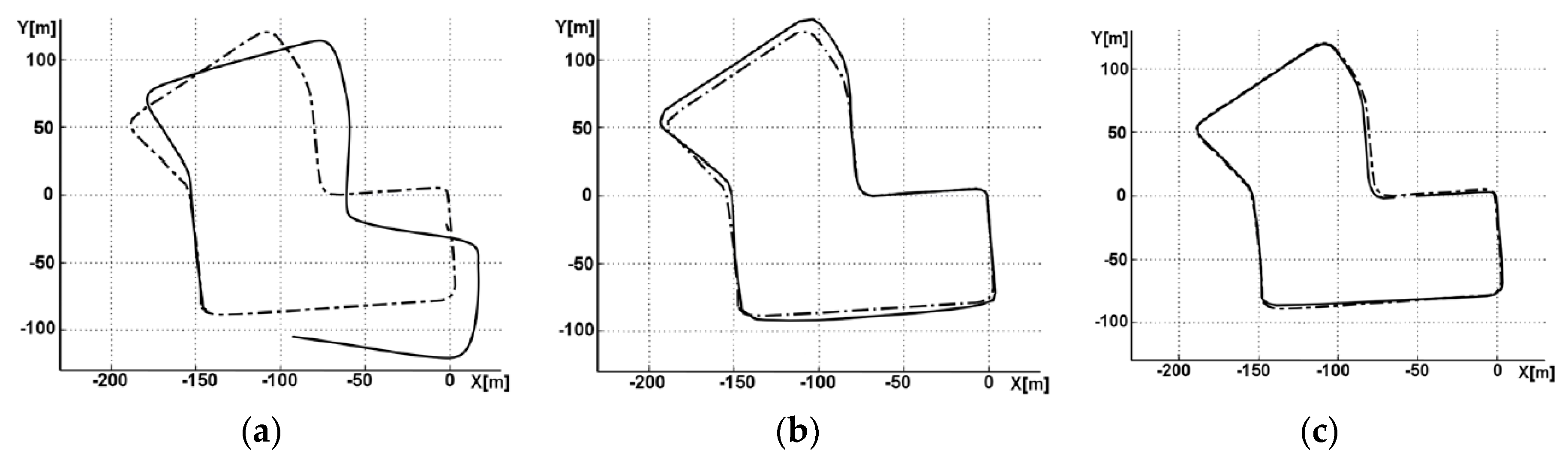
Figure 5а shows the result of using feature-based odometry from the ORB-SLAM system [
5,
6]. The maximum number of keypoints is limited to 100 to provide the required frame rate in case of onboard system without graphics processing unit (GPU) acceleration.
The analysis of
Figure 5а shows that the reconstructed trajectory has a significant error.
Figure 5b shows the result of using proposed model trained and tested on the same datasets. In this case, the error of reconstruction is much smaller.
Figure 5b shows the result of using feature-based odometry from ORB-SLAM with parallel correction based on the proposed model. As can be seen, the accuracy of the reconstruction is high.
Table 2 shows that the proposed approach performs a better trajectory reconstruction than the well-known ORB-SLAM. In particular, for sequence 7 from the KITTI dataset, the translation error of length is reduced by nearly 65.6% under the same frame rate (10 frames per second). Testing was carried out on the single-board Raspberry Pi 3+ Computer.
Figure 6a shows that the trained model on the KITTI-07 dataset has poor performance when tested on another dataset (KITTI-09).
Figure 6b shows that re-training of the model on the new dataset considerably increases the accuracy of the trajectory reconstruction from the dataset.
Thus, the results obtained on open datasets testify to the suitability of the model for practical use. To avoid overfitting, the complexity of model is optimized. However, the limited capacity of the optimized model requires its re-training when changing the domain area of use.
For an independent testing of trained model TUM set sequences shot outdoors were used. ORB-SLAM was tested on the same sequences with a limit of a 100 keypoints for comparison (
Table 3).
Analysis of
Table 3 demonstrates that ORB-SLAM translation error for TUM sequences exceeds the translation error of the proposed model more than 1.4 times. The ORB-SLAM rotation error exceeds the corresponding rotation error of the proposed model more than 2 times. Accuracy of the proposed model, however, tested on the independent sequence is lower than on the KITTI dataset, which was used in training, since at the beginning of TUM sequences indoor video footage, very different from the training data, was used.
Thus, the proposed model and training algorithm of the autonomous robot navigation system were tested on open datasets. Testing on the independent TUM sequence shot outdoors produces a translation error not exceeding 6% and a rotation error not exceeding 3.68 degrees per 100 m. Accuracy can be further improved by additional training on the samples of such sequences.


