1. Introduction
Many researchers build mathematical models and algorithms for price prediction [
1] or trend classification [
2]. For that, some of them used linear discrimination algorithms [
2] or regression algorithms like in [
3]. The aim of this work is to use statistical learning—part of artificial intelligence—to find profitable hours for trading. The work focuses on the currency market as a special case of financial markets, but it is extensible to other components such as stocks, commodities, etc. Volatility is a statistical measure of the dispersion of returns for a given market index or foreign exchange symbol. Volatility shows how quick the prices move, it can either be measured by using the standard deviation or variance between returns from that same security or market index. As explained in [
4], the bid–ask spreads or difference between the highest price and the lowest at a given time frame gives a dispersion measure. Commonly, the higher the volatility, the riskier the security. Volatility is influenced by many factors like liquidity, interest rate [
5], real estate [
6], opinions [
7], and a firm’s share. The authors in [
8] explain how liquidity providers of a market impact the volatility and stock returns, while the study in the paper [
6] re-examine the relationship between a firm’s market share and volatility.
This paper is an extended version of work published in [
9] that talks about volatility estimation. For that reason, let us first recall the main content of the previous work. It affirms that the financial markets calendar anomalies have been profoundly examined and contemplated finance professionals for a long time. Many artificial intelligence research also focuses on the financial market stability as an application. Let us talk about the factors that influence the asset prices. As introduced in [
10], the trading volume is the factor that investors have considered in the prediction of prices. It is a measure of the quantity of shares that change owners for a given financial product. For example, on the New York Stock Exchange known by “NYSE”, the daily average volume for 2002 was 1.441 billion shares, contributing to many billion dollars of securities traded each day among the roughly 2800 companies listed on the NYSE. The quantity of daily volume on a security can fluctuate on any given day depending on the amount of published—or known with different manner—information available about the company. This information can be a press releasex or a regular earnings announcement provided by the company, or it can be a third party communication, such as a court ruling, social networking like Twitter as explained in [
11], or a release by a regulatory agency pertaining to the company. The abnormally large volume was due to differences in the investors’ view of the valuation after taking in consideration the new information. Because of what can be inferred from abnormal trading volume, analysis of trading volume and associated price changes corresponding to informational releases has been of much interest to researchers. It is important for an investor or trader to study the stability factor of any market and many other factors that influence the prices like the interest rates [
12,
13], jobs, political stability, and more. Whatever it is, the difference between the highest and lowest asset values—that we will call a spread in this work—will be bigger when the prices are impacted by external and, perhaps unknown, factors.
This paper is organized as follows: the first section introduces related works. Since this paper is an extension of [
9], the related works section recalls the main guidelines explained in [
9]. In addition to that, we discuss—in the same section—the latests related works. The section “Approach Demystification” introduces the main definitions ad preliminaries in order to demystify the proposed approach. Next section untitled “MCMC Computational Model Building”—introduces the proposed hybrid model for volatility clustering. The use of mixture model combined with the density model is clarified in this section. Section “Testing and Discussion” show the obtained result on some symbols and discusses the homogeneity between the financial experts’ point of views and the approach results. Finally, the “Conclusion” recalls the main ideas and discusses the applications on algorithmic trading and financial data analysis.
2. Related Works
2.1. Existing Market Volatility Measurement
In trading, volatility is measured using certain indicators including average true range (ATR) and standard deviation. Moving averages (MA) and Bollinger bands are used for trend detection, but Bollinger bands can be used in volatility detection; the two bands diverging implies that the activity is starting (volatility). Each of these indicators can be used slightly differently to measure the volatility of an asset and interpret this data in a different format, but the computation of all those technical indicators uses continuous historical data that makes the signal noisy. Let us give an example; if the technical indicator is configured on the p-periods, the volatility measure at 14:00 is computed with p periods just before 14:00. In fact, this way of computation ignores all the events that happen at 14:00. This is why this computation must be done with the price’s variations of each 14:00 of the last p days.
2.2. Proposed Volatility Classifier Recall
In this sub-section, we recall the main content of the contribution [
9]. We consider the volume as one of the crucial parameters. The proposed algorithm will continuously supervise the evolution of the invested volume for each time frame (1 h in our case). To do so, let’s call
the
kth observed value of the volume at the hour
h. For example, if our data set contains the measures of one month, so we will have many values of the volume for the same hour
h: the volume today at 14 h is not necessarily the same yesterday at 14 h.
The stability of the forex market depends on the published news, their impacts, the behavior of the traders, and others [
12]. Actually, we do not have access to all those information and some are hidden. Some technical analysis like RSI (Relative Strength Index), MACD (Moving Average Convergence Divergence), and Moving Averages like in [
14] allows to detect some hidden intentions, but we believe that all those factors impact the variation and the evolution speed of the prices. In some period of the day, the same scenarios are repeated. The decision is really too hard and very fast for some time. However, the trends are somehow as expected for those pairs but for others hours, while the trading is not really interesting in some period of the day because the evolution is very slow. The trader will not loose and also will not win in this case. This is why we have to identify those clusters, and then the trader will choose the medium hours to trade. For that, we define the price spread
at the hour
h and the difference between the highest price and the lowest one of the same hour.
We have access to the volume, the prices and the highest and lowest prices archive. That allows our online learning algorithm to build the stability indicator for each hour. Let us suppose that we have
n observations for the hour
h stored in the learning data set:
. The stability estimator goal is mainly the study of the average behavior of the impact of the volume and spread on the price spread. We define the random variable
in (
1) as the vectorial average of all observations given the concerned hour
h. Formally:
2.2.1. Multivariate Probability Density
Let us focus now on the probability density of the random variable
that we defined in (
1). In probability theory, the central limit theorem—in the Vectorial Central Limit Theorem appendix—establishes that, when independent random variables are added, their sum converges to a Gaussian distribution even if those variables themselves do not follow a normal distribution.
Since the random variable
is defined in (
1) as an arithmetic mean and based on the theorem in
Appendix B, we have
. The probability density function of
is the bi-variate Gaussian and
is the determinant of the covariance matrix
.
2.2.2. Target Region Definition
Let be the volume target region; a set of medium volume values between and . We avoid all volumes less than because small values means the prices changes very slowly: that is to say, the trader will neither lose nor win. Greater volumes than implied a huge investment done by big investors or a collective decision done by the majority of the traders. Generally, this happens after an important economical or political announcement, those moments are risky and recommended to be avoided. Following the same reasoning, we define be the spread target region: a set of medium spread values between and . The final target region is in the next definition: .
2.2.3. Target Inclusion Probability
Since we have the density function of
but the target values of
, we have to transform those values to be adapted to
. Having
means that
because we have
. Based on that, let
and
be the transformed target regions for the new random variable
, where
and
are the arithmetic means of volume and spread respectively. In order to work with the density in Equation (
2), we have to use the transformed region
defined in (
3):
We can now move to the decision rule. In this subsection, we explain how the decision will be made; we can define the hypothesis
meaning that the financial market is stable and profitable (the market don’t moves slowly, no flash crashes and no high volatility (with a probability)). It holds if the
is in the target region:
. The opposite hypothesis
is hold and
is rejected when
. Holding
means that the trader have to avoid that risky trading at the hour
h. This probability is computed using the next formula
which is equal to
in (
7):
3. Preliminaries
3.1. Data Analysis
3.1.1. Data Set
The data comes streaming from some free web services or directly from a broker. In our case, we have used the platform MetaTrader—which is by default configured for GMT+2—to download the data sets. For each financial instrument, the data contains the seven main elements, the date, and time of each observation as a first component. The open and close prices that are the prices in the beginning and the end of each time frame (one hour in the context of this approach). Then the high and low prices that represents the highest and lowest variations of the price between the beginning and the end of the time frame. Finally, volume that represents the invested amount of money in that time frame. Our data set used in this paper contains non labeled historical spreads for each hour of the day. In order to avoid the confusion between the spread in our case and the spread as known in financial markets, let us call it a spread; the difference between the initial price (Open price described above) at the beginning of the hour and the price when the hour ends (Close price).
The second part of the analysis process is to filter the data set. By filtering we mean that we create a data set for each currency pair and each hour of the day. For example, if we want to study the EURUSD and USDCAD pairs at 14h (from 14:00 to 14:59), we select only the price spreads of that period for the two pairs.
3.1.2. Visualization and Observation
In this case, we have chosen the next currency pairs: EURUSD, EURGBP, GBPUSD, AUDCAD and NZDCHF. The same process can be applied to the others.
Table 1 shows some details about each currency pair above:
3.2. Approach Demystification
The idea behind the proposed approach in this paper, is in one hand, to estimate—for each hour of the day—the probability density function for the price spreads. then find for each traded symbol and for each hour of the day the. We recall that the price spread is the difference between the highest and the lowest price. That reflects the randomness of volatility [
15]—that is explained by many hidden events and information [
16]—during a specific time period.
Unsupervised anomaly detection is a fundamental problem in machine learning, with critical applications in many areas, such as cyber security, medical care, complex system management, and more. That inspires us to detect the activity class of currencies at a given time. The density estimation is in the core of activity detection: given a lot of input samples, activity corresponds to spreads that are residing in high probability density areas.
3.3. Main Definitions
The first step that is to be explained in this subsection is the stability regions meaning. The economical and political news announcements influence considerably financial market trends and sometimes the prices do not move considerably for many hours. This is why we have to define the values and as decision boundaries. In this paper, the computation is done with 5 pips for and 40 pips for . It means the less than 5 pips is considered a slow spread and more than 40 pips is a risky spread. See the region definition bellow:
Risk Region: , this region represents the the huge price spreads considered very risky. These are periods to avoid in order to minimize the risk to be a flash crash victim o any other quick spread due to economical or geopolitical events.
Slow Region: , this region represents the small price spreads that does not overpass the value that we can initialize with 5 pips for example.
Target Region: , is the best region that price spreads are normal and the trends can be kept for a while. Trading is recommended in this period.
3.4. Test on Experimental Data
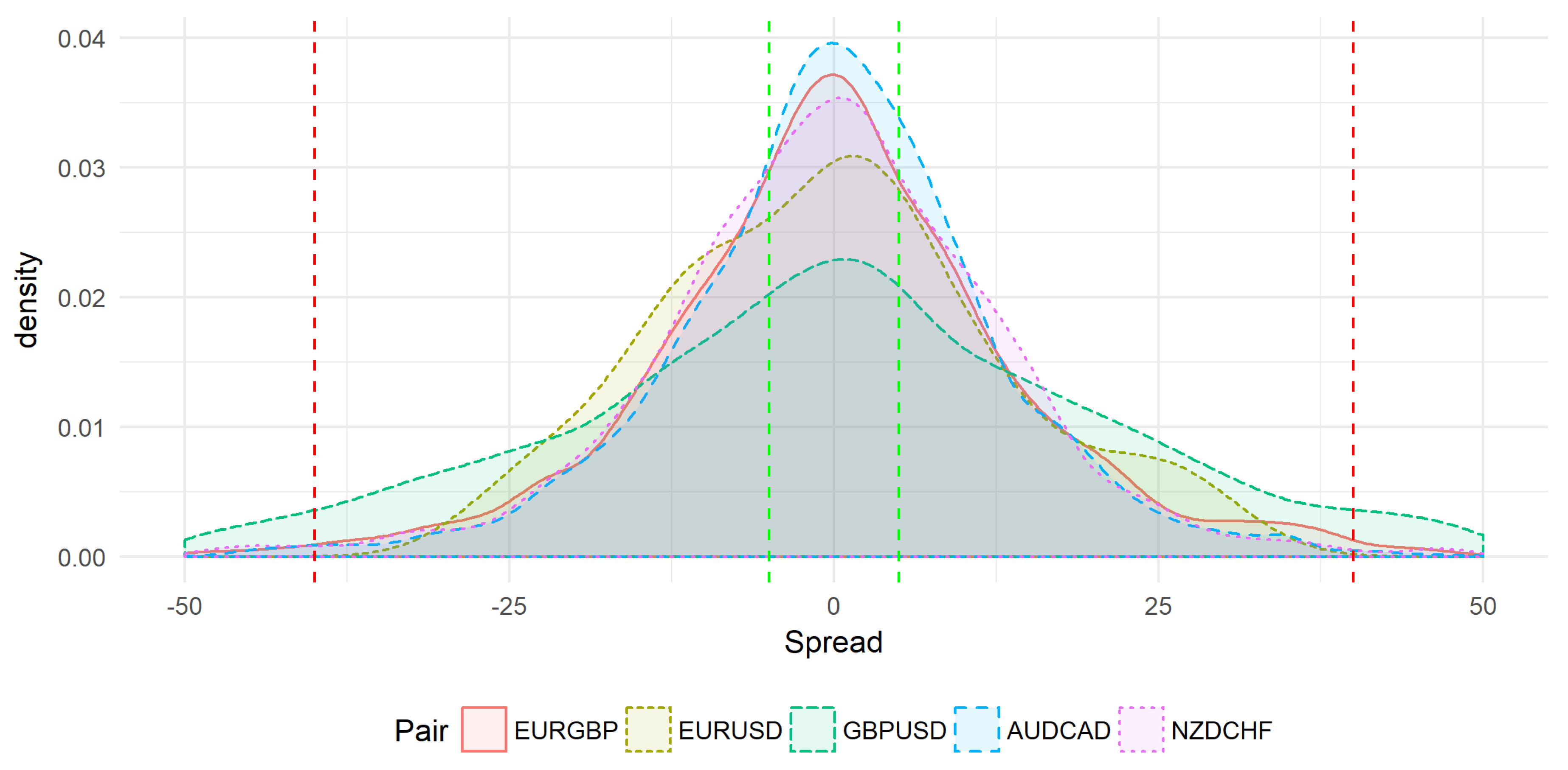
Using real experimental data,
Figure 1 shows the price spread distributions from 10:00 to 10:59. The plot allows us to do a comparative study between the behavior of many symbols from 10:00 to 10:59. This study is done for the symbols: EURGBP, EURUSD, GBPUSD, AUDCAD, and NZDCHF. Horizontal red lines represent the risk region delimited by
and
while horizontal green lines represent the values
and
. The goal is to estimate for the studied time (10:00 to 10:59, in this example), the probability that the spread (price spread) is concentrated in the target region
.
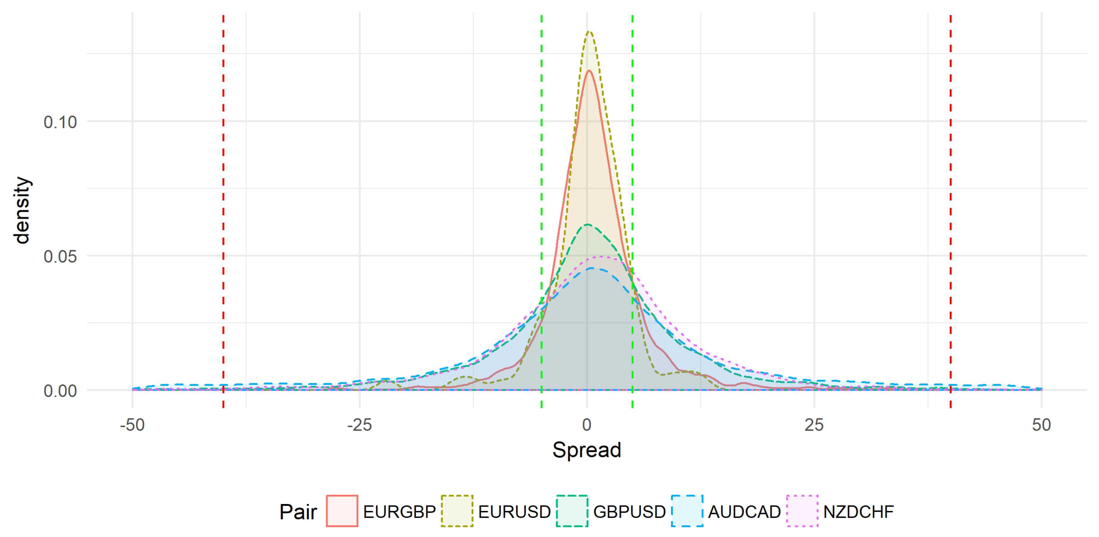
The same symbols are used in
Figure 2 but the time slot is different. In this case, collected data was in the range
to
. The volatility behavior seems to be different: most price spreads are concentrated in the slow region (
and
), between the two green lines.
4. MCMC Computational Model Building
In statistics, kernel density estimation—whose model is given in (
5)—is a non-parametric way to estimate the probability density function of a random variable [
17]. Kernel density estimation is a fundamental data smoothing problem where inferences about the population are made, based on a finite data sample.
In some fields such as signal processing and econometrics it is also termed the Parzen–Rosenblatt window method, after Emanuel Parzen and Murray Rosenblatt, who are usually credited with independently creating it in its current form. Gaussian kernel is used in our approach, it is given by the Equation (
6) bellow:
The goal is to compute the probability that the symbol behavior—represented by the spread
m—is in the target region
as defined before. That comes to compute the integral of the estimated density
—in (
5)—all over
.
In order to compute the Gaussian integral, we rely on Monte Carlo simulation as it is applied in [
18,
19,
20]. Let us generate a sample
from a uniform distribution in the target region
. The sample size is
, it is better to be big as possible (
). The computation of the probability
as defined in (
7) approximated using Monte Carlo stochastic method for numerical integrals computation. This method affirms that
converges to the desired value
. With
is the spread of target region
. It is formally given by
. By combining the Equations (
5)–(
7) we obtain:
Figure 3 shows the obtained target region inclusion probabilities for each hour of the day. The computations is done for many symbols at the same time in order to compare the best hours for each symbol.
5. Gaussian Mixture Model
5.1. Mixture Model Building
In statistics, a mixture model is a probabilistic model for representing the presence of sub-populations within an overall population, without requiring that an observed data set should identify the sub-population to which an individual observation belongs. Formally, a mixture model corresponds to the mixture distribution that represents the probability distribution of observations in the overall population [
17,
21]. However, while problems associated with “mixture distributions” relate to deriving the properties of the overall population from those of the sub-populations, “mixture models” are used to make statistical inferences about the properties of the sub-populations given only observations on the pooled population, without sub-population identity information.
Let us suppose that we have K component indexed by j. A finite mixture of K densities of the same distribution is a convex combination of previous densities weighted by . Let be the finite mixture, and let’s call the mixture parameters set that we rewrite simply .
5.2. Likelihood Function and Missing Data
Paper [
22] affirms that when the observations can be seen as incomplete data, the general methodology used in finite Gaussian mixture involves the representation of the mixture problem as a particular case of maximum likelihood estimation (MLE). This setup implies consideration of two sample spaces, the sample space of the (incomplete) observations, and a sample space of some complete observations, the characterization of which being that the estimation can be performed explicitly at this level, as explained in [
22]. For instance, in parametric situations, the MLE based on the complete data may exist in closed form. Among the numerous reference papers and monographs on this subject are, e.g., the original EM algorithm - in
Appendix A - and the finite mixture model book and references therein. We now give a brief description of this setup as it applies to finite mixture models in general. The observed data consist of
n i.i.d. observations
from a density
by (
9).
In order to simplify the likelihood, we can introduce latent variables
such that:
and
is the prior probability of
going to cluster
j. These auxiliary variables allows us to identify the mixture component each observation has been generated from. The mixture, in (
9), with hidden variable
becomes
:
With
is equal to 1 if the condition
is hold and 0 if not. The log-likelihood, that we denote here with
, is given by the quantity
. Equation (
11) shows the final likelihood expression:
6. Results and Discussions
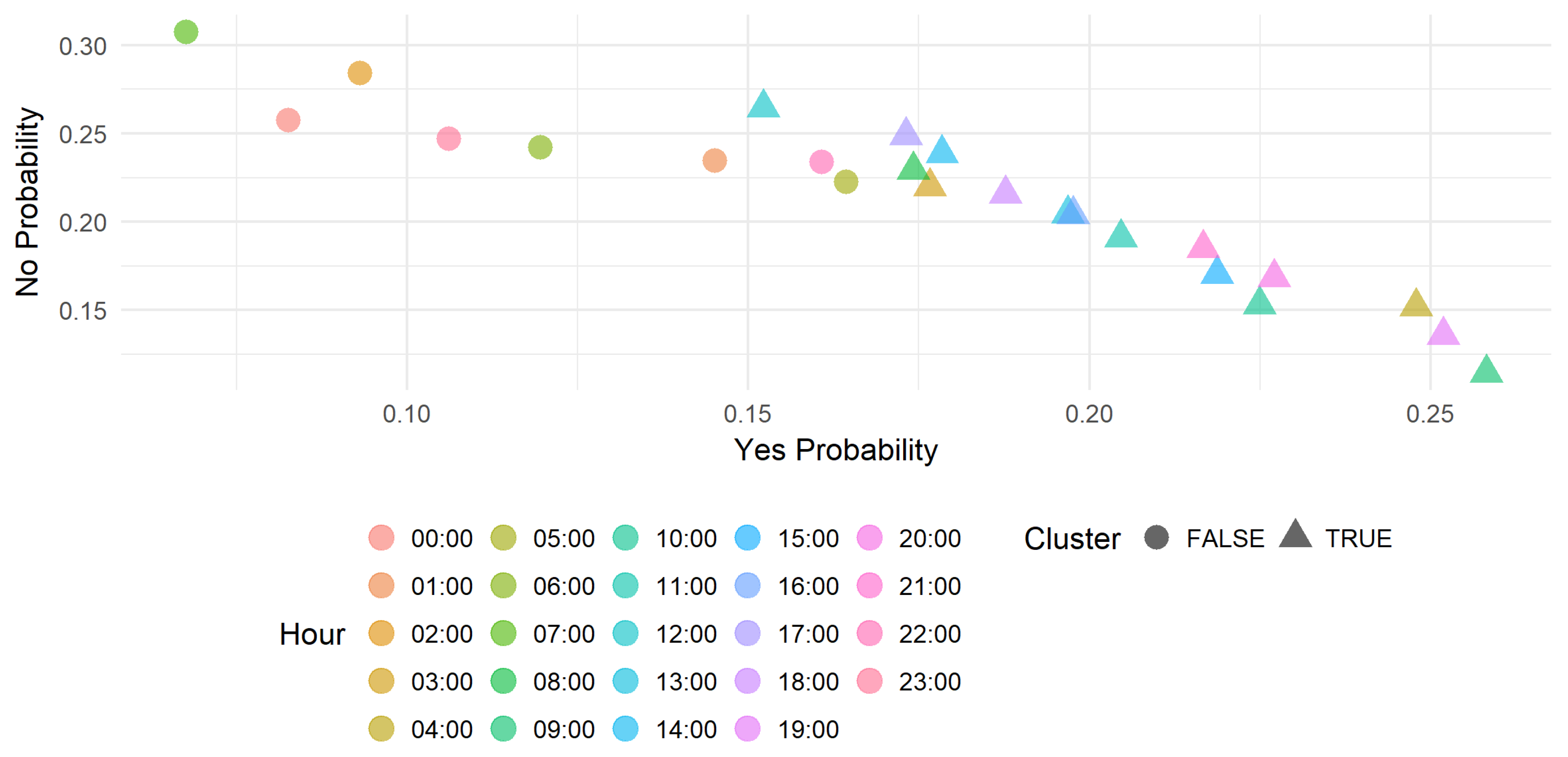
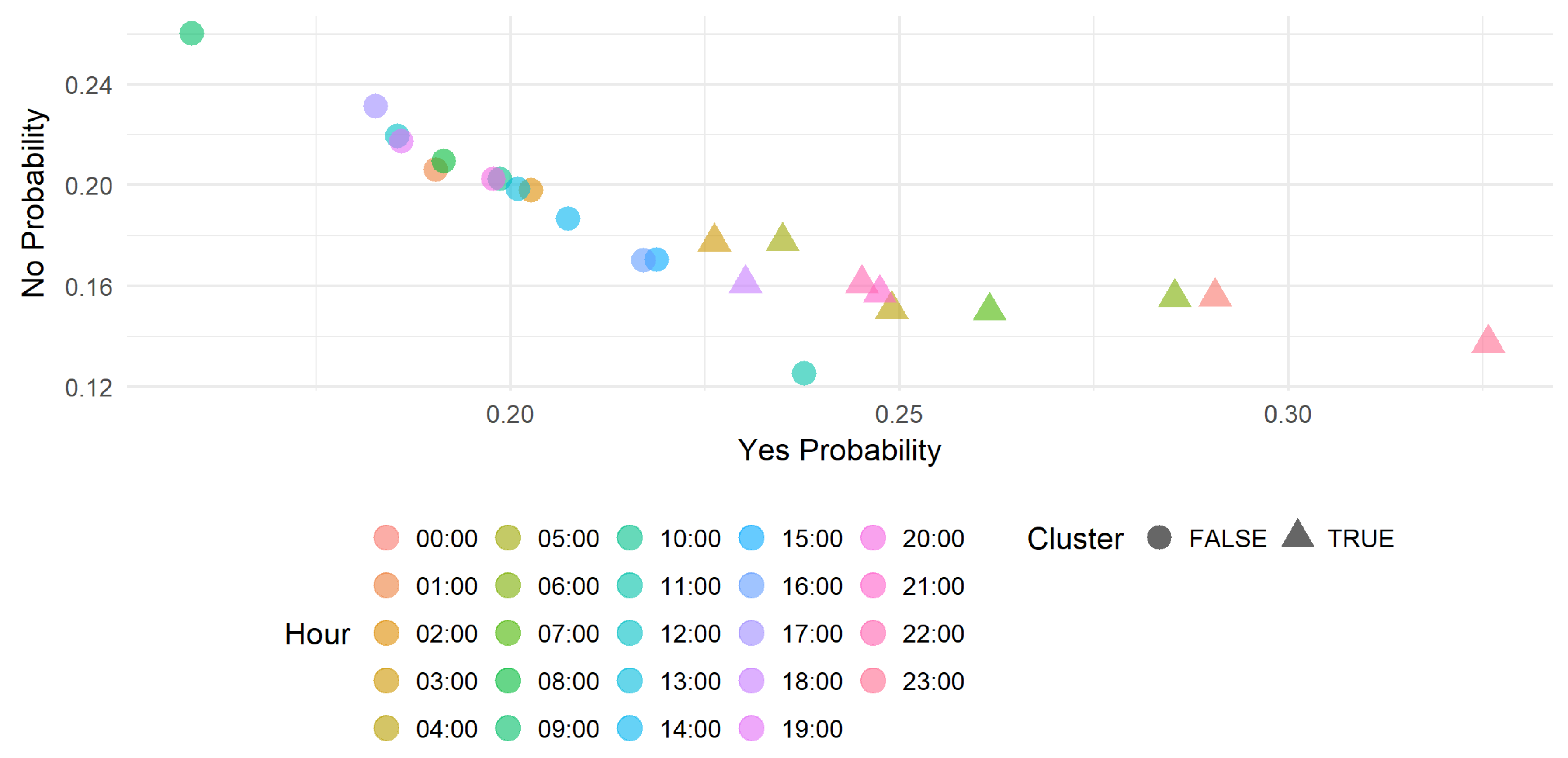
This section presents obtained results visualized in scatter plots.
Figure 4 and
Figure 5 show the profitability of the trade on the EURUSD and NZDCHF symbols during 24 h of the day. Each data point represent the Yes (Trade it) and No (do not) probabilities and the cluster obtained with Gaussian mixture. The scatter points format (circle or triangle) represents the cluster and differentiates the hours to on which it is recommended to trade the symbol and those on which is not recommended. In this case, the triangle represents the positive cluster then recommends to trade the symbol.
We can select only a subset of hours that concerns the trader and run this recommendation approach. That allows the trader to manage his scheduling with more flexibility. The concept can be integrated also in a trading robot implementing a strategy that can fail with small or very hight volatility.
7. Conclusions
In this paper, we presented a currency market volatility estimator and proposed computational model relies on Gaussian mixture model combined with the Gaussian kernel density. We have defined three classes for the volatility variation: the slow region, target region, and the risky region. The main goal of the proposed approach is to measure—for each hour of the day—the probability that a currency activity is included in a given region. The proposed model has a range of applications in financial markets. On one hand, its implementation in a platform like MetaTrader allows the trader to predict the symbol activity instantaneously; in other words, the trader can select profitable symbols at each hour of the day. On the other hand, the model can be implemented in a trader robot in order to find sufficient volatility to run a given strategy. This work is supported by real data analysis and results confirm that the model has an equivalent level of accuracy close to that of financial professionals.
The Monte Carlo method is used to compute the integrals in this approach. Computational aspects of this method need deep thinking in further works. As perspectives, a comparative study in computational complexity and accuracy has to be done between the different sampling methods such as Metropolis Hasting, Gibbs sampling and Monte Carlo Markov Chain. Profitable zone upper and lower bounds have been established as percentage in order to do the study. The models in this paper will be implemented in a real technical indicator embedded in MetaTrader platform. Profitable zone parameters will be considered as two inputs that will be given by the user according to the sensitivity that he want. Since there are some strategies that need high volatility to be profitable, we can do another study specially to find the values for different trading styles as a perspective.
We think that artificial intelligence-driven algorithmic trading is the future of financial markets. For that reason, further works will focus on the design of expert system—trading robot, or expert advisor as we call it in the MetaQuote community—that uses machine learning for the prices and trends prediction triggered with the result of the volatility estimator in this work. We believe that this collaborative distributed intelligence can produce a kind of trading robot.
We express our strong belief that a data and artificial intelligence cross disciplinary approach will give the algorithmic trading a new momentum. Finally, we hope that this work will contribute on the development of this arising field.
Author Contributions
Conceptualization, S.T.; Formal analysis, S.T.; Investigation, S.T.; Methodology, S.T.; Resources, R.S.; Visualization, S.T.; Writing—review and editing, H.C.
Funding
This research received no external funding.
Acknowledgments
I would like to thank the anonymous referees for their valuable comments and helpful suggestions. Special thanks goes to any one that improved the language’s quality and made this paper more readable.
Conflicts of Interest
I declare that I have no conflict of interest and no financial or other interest with any entity to disclose.
Abbreviations
The following abbreviations are used in this manuscript:
| FX | Foreign Exchange |
| MCMC | Monte Carlo Markov Chain |
| GMM | Gaussian Mixture Model |
| EM | Expectation Maximization |
Appendix A. EM Algorithm
The expectation maximization algorithm or EM algorithm, is a general technique for finding maximum likelihood solutions for probabilistic models having latent variables. Here we give a very general treatment of the EM algorithm for Gaussian mixtures does indeed maximize the likelihood function.
In the special case of Gaussian components, the parameters update procedures are given by the expressions in (
A4):
Appendix B. Multivariate Central Limit Theorem
If , ..., are independent and identically distributed with mean and covariance having finite entries, then: .
References
- Al-askar, H.; Lamb, D.; Hussain, A.J.; Al-Jumeily, D.; Randles, M.; Fergus, P. Predicting financial time series data using artificial immune system inspired neural networks. Int. J. Artif. Intell. Soft Comput. 2015, 5, 45–68. [Google Scholar] [CrossRef]
- Tung, H.H.; Cheng, C.C.; Chen, Y.Y.; Chen, Y.F.; Huang, S.H.; Chen, A.P. Binary Classification and Data Analysis for Modeling Calendar Anomalies in Financial Markets. In Proceedings of the 7th International Conference on Cloud Computing and Big Data (CCBD), Macau, China, 16–18 November 2016. [Google Scholar]
- Chirilaa, V.; Chirilaa, C. Financial market stability: A quantile regression approach. Procedia Econ. Financ. 2015, 20, 125–130. [Google Scholar] [CrossRef]
- Blau, B.M.; Griffith, T.G.; Whitby, R.J. The maximum bid-ask spread. J. Financ. Mark. 2018. [Google Scholar] [CrossRef]
- Hajilee, M.; Niroomand, F. The impact of interest rate volatility on financial market inclusion: Evidence from emerging markets. J. Financ. Mark. 2018, 42, 352–368. [Google Scholar] [CrossRef]
- Anoruo, E.; Vasudeva, N.R.M. An examination of the REIT return–implied volatility relation: A frequency domain approach. J. Financ. Mark. 2016, 41, 581–594. [Google Scholar] [CrossRef]
- Mehmet, B.; Riza, D.; Rangan, G.; Mark, E.W. Differences of opinion and stock market volatility: Evidence from a nonparametric causality-in-quantiles approach. J. Financ. Mark. 2017, 42, 339–351. [Google Scholar] [CrossRef]
- Chung, K.H.; Chuwonganant, C. Market volatility and stock returns: The role of liquidity providers. J. Financ. Mark. 2017, 37, 17–34. [Google Scholar] [CrossRef]
- Tigani, S.; Saadane, R. Multivariate Statistical Model based Currency Market Proftability Binary Classifer. In Proceedings of the 2nd Mediterranean Conference on Pattern Recognition and Artifcial Intelligence, Rabat, Morocco, 27–28 March 2018. [Google Scholar]
- MIT Laboratory for Information and Decision Systems. Relationship between Trading Volume and Security Prices and Returns; Tech. Rep. P-2638; Massachusetts Institute of Technology: Cambridge, MA, USA, 2013. [Google Scholar]
- Kanungsukkasem, N.; Leelanupab, T. Finding potential influences of a specific financial market in Twitter. In Proceedings of the 7th International Conference on Information Technology and Electrical Engineering (ICITEE), Chiang Mai, Thailand, 29–30 October 2015. [Google Scholar] [CrossRef]
- Fouejieu, A. Inflation targeting and financial stability in emerging markets. Econ. Model. 2017, 60, 51–70. [Google Scholar] [CrossRef]
- Adjei, F.; Adjei, M. Market share, firm innovation, and idiosyncratic volatility. J. Financ. Mark. 2016, 41, 569–580. [Google Scholar] [CrossRef]
- Branquinho, A.A.B.; Lopes, C.R.; Baffa, A.C.E. Probabilistic Planning for Multiple Stocks of Financial Markets. In Proceedings of the IEEE 28th International Conference on Tools with Artificial Intelligence (ICTAI), San Jose, CA, USA, 6–8 November 2016. [Google Scholar] [CrossRef]
- Bui Quang, P.; Klein, T.; Nguyen, N.H.; Walther, T. Value-at-Risk for South-East Asian Stock Markets: Stochastic Volatility vs. GARCH. J. Risk Financ. Manag. 2018, 11, 18. [Google Scholar] [CrossRef]
- Tegnér, M.; Poulsen, R. Volatility Is Log-Normal But Not for the Reason You Think. Risks 2018, 6, 46. [Google Scholar] [CrossRef]
- Alam, M.D.; Farnham, C.; Emura, K. Best-Fit Probability Models for Maximum Monthly Rainfall in Bangladesh Using Gaussian Mixture Distributions. Geosciences 2018, 8, 138. [Google Scholar] [CrossRef]
- Wang, Y.; Infield, D. Markov Chain Monte Carlo simulation of electric vehicle use for network integration studies. Int. J. Electr. Power Energy Syst. 2018, 99, 85–94. [Google Scholar] [CrossRef]
- Kaiser, W.; Popp, J.; Rinderle, M.; Albes, T.; Gagliardi, A. Generalized Kinetic Monte Carlo Framework for Organic Electronics. Algorithms 2018, 11, 37. [Google Scholar] [CrossRef]
- Marnissi, Y.; Chouzenoux, E.; Benazza-Benyahia, A.; Pesquet, J.C. An Auxiliary Variable Method for Markov Chain Monte Carlo Algorithms in High Dimension. Entropy 2018, 20, 110. [Google Scholar] [CrossRef]
- Li, J.; Nehorai, A. Gaussian mixture learning via adaptive hierarchical clustering. Signal Process. 2018, 150, 116–121. [Google Scholar] [CrossRef]
- Benaglia, T.; Chauveau, D.; Hunter, D.R.; Young, D.S. mixtools: An R Package for Analyzing Mixture Models. J. Stat. Softw. 2010, 32, 1–29. [Google Scholar] [CrossRef]
© 2019 by the authors. Licensee MDPI, Basel, Switzerland. This article is an open access article distributed under the terms and conditions of the Creative Commons Attribution (CC BY) license (http://creativecommons.org/licenses/by/4.0/).


