Article

Statistical Modeling of Trivariate Static Systems: Isotonic Models

1
Dipartimento di Ingegneria dell’Informazione, Università Politecnica delle Marche (UnivPM), 60131 Ancona, Italy
2
School of Information and Automation Engineering, Università Politecnica delle Marche (UnivPM), 60131 Ancona, Italy
*
Author to whom correspondence should be addressed.
These authors contributed equally to this work.
Submission received: 27 November 2018 / Revised: 9 January 2019 / Accepted: 17 January 2019 / Published: 21 January 2019

Abstract

:
This paper presents an improved version of a statistical trivariate modeling algorithm introduced in a short Letter by the first author. This paper recalls the fundamental concepts behind the proposed algorithm, evidences its criticalities and illustrates a number of improvements which lead to a functioning modeling algorithm. The present paper also illustrates the features of the improved statistical modeling algorithm through a comprehensive set of numerical experiments performed on four synthetic and five natural datasets. The obtained results confirm that the proposed algorithm is able to model the considered synthetic and the natural datasets faithfully.

1. Introduction

The availability of large datasets in the scientific literature calls for novel and efficient algorithms to build models that are potentially able to explain the complex non-linear relationships between attributes [1]. Examples of diverse publicly available datasets published in the Data journal are [2,3,4,5,6,7,8,9], which range from protein synthesis data to human body movements acquisitions. Non-linear modeling is ubiquitous in applied sciences and engineering, as in agriculture, forestry and finance [10,11,12,13,14,15].
Several applications in sciences and engineering rely on inferring a relationship between a dependent variable z R and a pair of independent variables ( x , y ) R 2 on the basis of a number of joint observations of these three variables’ values. This kind of modeling is termed trivariate. Illustrations come, for example, from materials science [16], where the elasticity (independent variable) of a polypropilene composite reinforced with natural fibers is modeled in terms of the geometric characteristics, namely length and diameter (independent variables) of the embedded fibers, as well as from bioenergy analysis [17], where the smoke emission of a compression ignition engine fed with biomass-derived fuel is modeled in terms of injection timing and biomass blend ratio. Further illustrations are found in [18], where the effects of pharmacological interventions that modulate calcium ions homeodynamics and membrane potential in rat isolated cerebral vessels during vasomotion were simulated by a three-variable non-linear model, as well as in [19], where the performance of habitat suitability models for macrophytes was assessed in terms of temperature, acidity and conductivity.
A data-driven multivariate model is a combination of inferences based on collected data used to predict information. A model can be an equation or a numerical-table-based representation of information. The applications of non-linear multivariate models are numerous, ranging from control system design [20] to early disease diagnosis [21] and to college-level student performance prediction [22]. In general, data-driven models are used to replace actual physical systems to test hypotheses and to help inferring phenomena that cannot be observed directly [1]. A noteworthy example is found in simulated drug testing (see, e.g., [23]), where a model is used to predict the effects (and the side effects) of a drug in treatment, in place of actual patients’ treatment. Model-based prediction can also be applied to data dimensionality reduction [24].
Trivariate modeling consists in inferring a model z = f ( x , y ) , on the basis of a number of observed triples ( z s , x s , y s ) , s = 1 , , S , where S denotes the total number of observations [25]. The triples of values ( z s , x s , y s ) collected in the experimental setting may be affected by measurement errors and the dependency between the three variables may be affected by nuisance variables that are not taken into account in the modeling process. In this context, the trivariate modeling process may take advantage of statistical information, obtained by pooling the available observations { ( z s , x s , y s ) } s = 1 , , S . This paradigm is termed statistical modeling (see, e.g., [26,27,28]), in contrast to deterministic non-linear modeling that use the default least squares loss function or a custom loss function to fit models and that minimizes the sum of the loss function across the observations.
A specific modeling problem arises whenever it is known, from the nature of the phenomenon described by three variables, that the underlying relationship between the dependent variable and the two independent variables is monotonic. Examples of such situations occur, e.g., in food toxicology research [29], where it was observed that the concentration of acrylamide (dependent variable) produced in the process of cooking French fries increases monotonically with cooking time and temperature (independent variables), in air quality surveillance [30], where it was found experimentally that the concentration of carbon dioxide dispersed in the air grows monotonically with the concentrations of nitric oxide and of benzene, as well as in [31], which applies trivariate isotonic modeling to urbanisation and life expectancy data and to study the impact of the neighborhood share of high skilled residents on local property prices in the United Kingdom. A model that embodies the feature of monotonic dependency is termed isotonic model (see, e.g., [32]).
The Letter [33] introduced a novel instance of trivariate statistical isotonic modeling. The introduced method requires the estimation of the second-order joint probability density functions p x , y and p z , y and is based on a probability conservation law of statistics, that constraints the shape of the sought model f. The joint probability density functions of the independent variables and of the dependent/independent variables should match each other in a unique way, that determines the shape of the model. An interesting feature of this method is that all the required quantities are stored in numerical tables, including the model itself which is therefore represented as a numerical table, and the mathematical operations required to infer the model are simple additions/multiplications and table search.
From an alternative viewpoint, the Letter [33] suggested a method for the re-sampling of a function f ( x , y ) of two independent variables, provided that the function is monotonically increasing and a sufficiently large number of data points ( z s , x s , y s ) are available. The sequence ( z s , x s , y s ) can be in a random order and not necessary matching the mesh ( x i , y j ) at which z i j = f ( x i , y j ) is evaluated by the re-sampling.
In the Letter [33], a first implementation was proposed and a numerical test was conducted on a synthetic dataset. The present contribution builds on the Letter [33] by refining the software implementation proposed thereby in three specific ways:
  • by taking in better account ‘the border effects’ at the periphery of the mesh: this improvement will lead to more accurate model inference results at the periphery of the data-domain;
  • by filling-in empty bins of the numerical, histogram-based, estimations of the joint probability density functions p x , y and p z , y with small non-zero values: this improvement to the original algorithm solves the problem of missing statistical information in some areas of the data-domain mostly due to the scarcity of data samples in those areas;
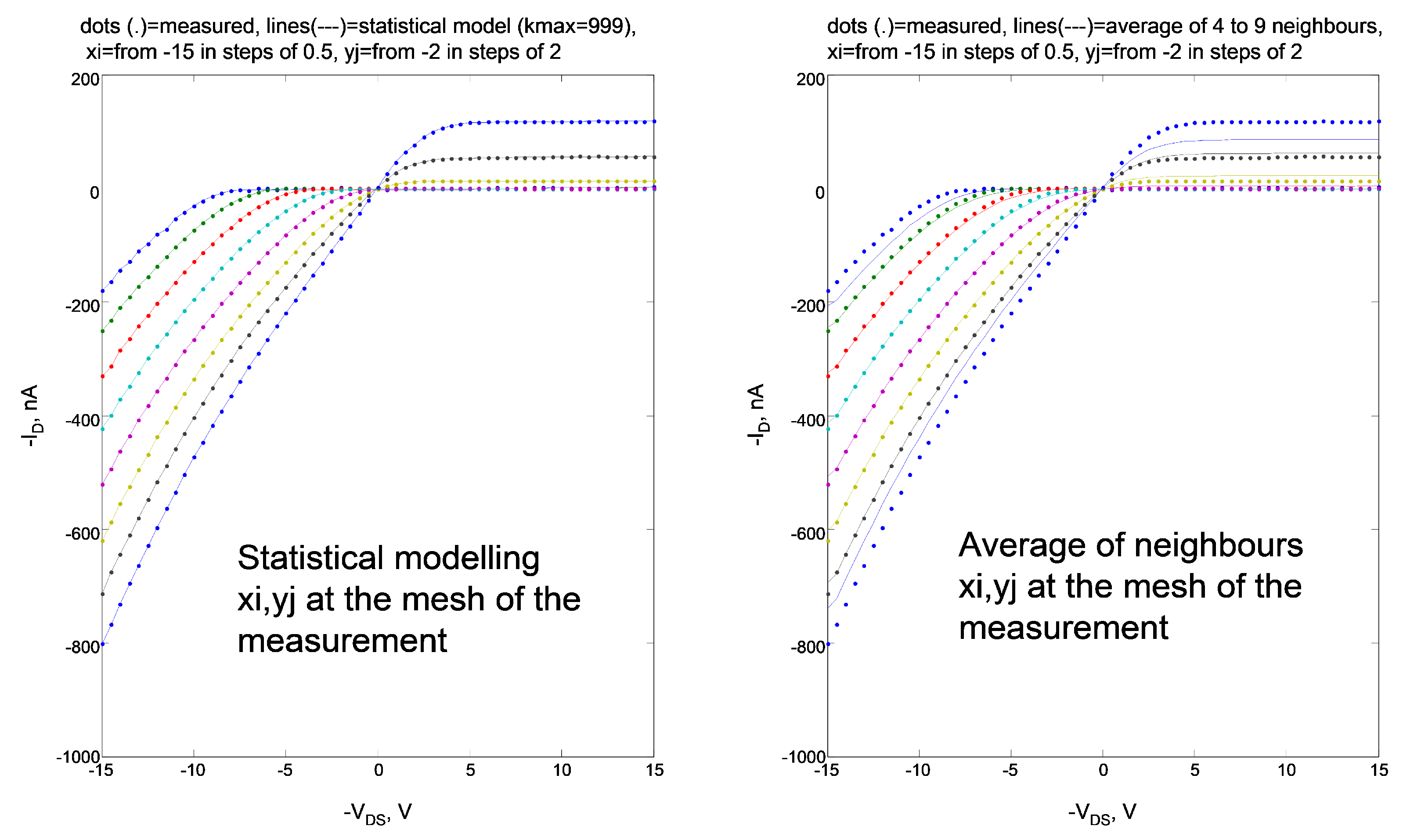
  • by smoothing out the inferred model through linear interpolation by neighboring values: this improvement over the original version of the algorithm mitigates the discontinuity of the model due to a discretized meshing of the data-domain.
The present paper is organized as follows. The principles informing the proposed statistical isotonic modeling technique are recalled in the Section 2, which also explains implementation details of the proposed procedure versus the one presented in [33]. The Section 3 presents several numerical tests, conducted either on synthetic data and on real-world data, to evaluate the proposed modeling technique. The Section 4 concludes the paper.

2. Modeling Principle and Implementation Details

Let x , y R 2 denote two continuous random variables with joint probability density function p x , y : R 2 R + and let f : R 2 R denote a regular function (with a slight abuse of notation, we confuse a random variable with its realizations). The function f is continuous, with continuous first-order partial derivatives and it is assumed that f x > 0 . Define the random variables pair ( z , v ) = def ( f ( x , y ) , y ) . These new random variables are continuous and their joint probability density function is denoted by p z , v : R 2 R + .
The relationship between the probability density functions p x , y and p z , v is given by [34]:
p z , v = p x , y z x v y z y v x .
Recalling that v = y and the assumption on monotonicity, the above relationship becomes:
p z , y f x = p x , y .
In the context of statistical modeling, the joint probability density functions p x , y and p z , v are estimated by pooling the available observations { ( z s , x s , y s ) } s = 1 , , S . Hence, the above equation has the model f as only unknown. Upon introducing the integrals
P x , y ( x , y ) = def x p x , y ( ζ , y ) d ζ , P z , y ( z , y ) = def z p z , y ( ζ , y ) d ζ ,
which represent marginal cumulative distribution functions of the random-variable pairs ( x , y ) and ( z , y ) , respectively, the solution to the Equation (2) may be expressed, in intrinsic form, as:
P z , y ( f ( x , y ) , y ) = P x , y ( x , y ) .
Upon fixing a pair of values ( x , y ) , the left-hand term of the solution (4) is an invertible function of the unknown f ( x , y ) , while the right-hand term is a known value. Hence, for any fixed pair of values ( x , y ) , the corresponding value of the model f ( x , y ) may be found by function inversion.
The above principle to build a model f needs to be converted into a numerical algorithm suitable for the processing of a finite set of data triples. The Section 2.1 recalls the main details of the implementation suggested in [33], while the Section 2.2 presents a refinement of the earlier implementation which takes in better account the border effects at the periphery of the mesh, fills-in empty bins of the numerical estimations of the joint probability density functions p x , y and p z , y , and smooths out the inferred model through interpolation by neighboring values.

2.1. Details on an Earlier Implementation

We recall here the principal details about the MATLAB implementation proposed in an earlier contribution [33]. The probability density functions p x , y and p z , y are estimated through normalized occurrence histograms [35] and are represented by numerical look-up tables (see, e.g., [36]). The integrals P x , y ( x , y ) and P z , y ( z , y ) are, in turn, approximated by cumulative sums and are likewise represented by numerical look-up tables. For every given point ( x , y ) of the look-up table that represents this pair of variables, the model value f ( x , y ) is estimated as the unique z-value that minimizes the quantity | P z , y ( z , y ) P x , y ( x , y ) | . Such z-value was sought through a proximity search on a row of the table that represents the quantity P z , y ( z , y ) [33]. The corresponding non-iterative computational procedure, written in MATLAB language, is shown in Figure 1.
The procedure shown in Figure 1 inputs the triples ( z s , x s , y s ) as three arrays z, x and y, each of length S, and returns a pair of vectors, namely xg and yg, and a matrix zz that represents the estimated model. The number of subdivisions for probability density function estimation coincides with the number of partitions of the x, y and z axes for model estimation. (This procedure may be modified to make the finesse of partition for probability density function estimation and the number of partitions of the x, y and z axes for model estimation be independent.) In the code excerpt of Figure 1, the instruction hist3 serves to estimate the joint probability density function of two variables by a histogram method, while the instruction cumsum serves to estimate the cumulative distribution function with respect to one of the variables.
In the lines 01–03, the algorithm inputs the three arrays z, x and y, computes their range and the bin widths w x , w y and w z according to the following formulas:
w x = def σ x S 4 , w y = def σ y S 4 , w z = def σ z S 4 ,
where the sample standard deviation σ x of the x-variable is computed by the unbiased estimator
σ x = def s = 1 S x s x ¯ 2 S 1 ,
where x ¯ denotes the mean value of the x-variable, and likewise for σ y and σ z .
The line 04 defines the arrays xg, yg and zg, which represent the sampling points over a three-dimensional grid according to the above-defined bin-sizes. The obtained arrays read:
xg = def x min , x min + w x , x min + 2 w x , xg j , , x min + ( S x 1 ) w x ,
yg = def y min , y min + w y , y min + 2 w y , yg i , , y min + ( S y 1 ) w y ,
zg = def z min , z min + w z , z min + 2 w z , zg k , , z min + ( S z 1 ) w z ,
where S x , S y and S z denote the size of each array that are computed in the line 05.
The lines 06–07 estimate the probability density functions pzy and pxy through the MATLAB function hist3. For instance, for the joint probability density pxy, such function inputs the arrays x and y and the bins-numbers S x and S y and computes the joint occurrence histogram, namely, returns an array of size S y × S x which, in the ( i , j ) -th cell contains the number of pairs ( y s , x s ) such that x s falls within the j-th bin of the x-grid and y s falls within the i-th bin of the y-grid. In addition, the lines 06–07 normalize the estimated occurrence histograms over the total number of samples and over the bins-widths and computes the arrays xPxy and zPzy, through the MATLAB function cumsum. These two arrays represent the cumulative distribution functions approximated over the discrete grid.
Subsequently, for any row (of index i) of the arrays xPxy and zPzy, the computer code evaluates which element (of index k) of the array zPzy is the closest to the j-th element of the array xPxy by the lines 09–14. Once the index k has been determined, the computer code assigns the value zg ( k ) to the ( i , j ) -th element of the array zz. The array zz will represent the built model.
In order to emphasize the criticalities emerged from the discussed method, we have carried out some performance evaluation also in comparison with another method for black-box modeling that uses averaging of 4–64 neighboring points [37]. This evaluation confirms that the proposed method is 5–10 times faster than the other method, but the accuracy of the statistical modeling method is worse, approximately 3 times worse than the accuracy of method of averaging of the near neighbors.
The Figure 2, Figure 3 and Figure 4 compare the statistical modeling with the method of average of neighbors on a natural dataset. These measured data concern an organic TFT and are drawn from the study [38]. (Organic thin-film transistor (OTFT) technology involves the use of organic semiconducting compounds in electronic components, notably computer displays; several factors have motivated engineers to conduct and continue research in organic semiconductor technology, one of which is cost.) Note that data with inverted polarity are used for modeling, since the particular TFT is a p-type field-effect transistor. Therefore, I D and V D S are at the axes of the figures. In this experiment, the number of partitions of the z axis is denoted by k max .
In Figure 2, the grid was chosen to be at the measured data points. The results of this experiment confirm that the statistical modeling can be made accurate, if performed on the mesh of the measurement, while the average of neighbors fails in this case.
In Figure 3 and Figure 4, the step and position of the points were chosen not to coincide with the mesh of the measured data. The Figure 3 shows how the statistical modeling shifts on the right, if the grid value x j is chosen in-between the x s values of the measurement. The average of neighbors works well in the left-hand side for negative values of I D , but fails when the values of I D are not equally spaced in the y-value. The ‘shift on the right’ effect encountered in statistical modeling likely is due to the method of searching for the minimum of | P z , y P x , y | , and the shift could be on the left, if the mesh-grid for x j is shifted oppositely.
The Figure 4 shows that re-sampling at y i between the mesh-grid of the y s values of the measurement, the lines of the model should be between the dots of the measurement, as seen for the average of neighbors in the right-hand plot. The statistical modeling fails by re-sampling y i not at the mesh-grid of the y s values of the measurement. For the negative I D , the statistical modeling repeats z s , instead of being between z s of neighboring y s . For the positive I D , the statistical modeling again repeats z s .

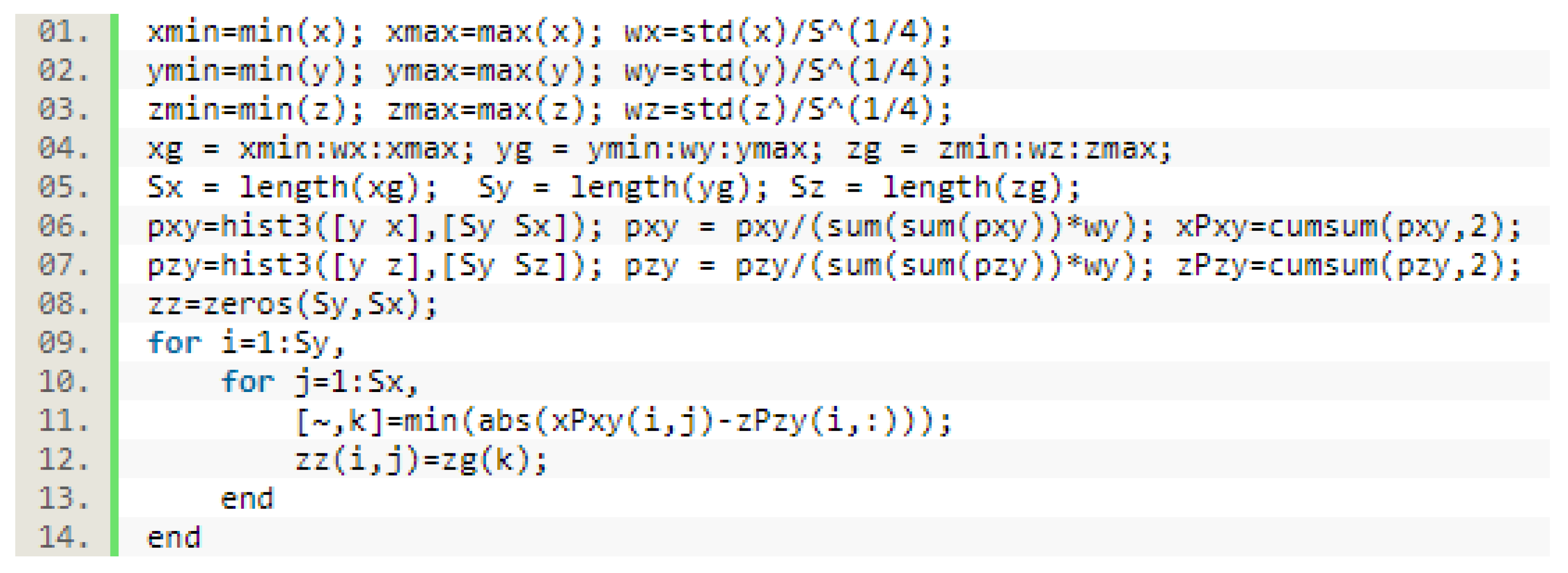
2.2. Refined Implementation

The first refinement introduced in the present paper is about the arrays xg, yg and zg. Such arrays may be realized by first estimating the widths of the intervals through which the histograms will be constructed, in order to obtain an approximated number of intervals, S x , S y and S z ; such widths, upon rounding, will give the effective widths w x , w y and w z . Thus, since the estimated probability in any interval is assigned to its mid value, the arrays xg, yg and zg, are re-defined as follows:
xg = def x min + w x 2 , x min + w x , , xg j , , x max w x 2 ,
yg = def y min + w y 2 , y min + w y , , yg i , , y max w y 2 ,
zg = def z min + w z 2 , z min + w z , , zg k , , z max w z 2 .
These three arrays count a number S x + 1 , S y + 1 and S z + 1 of elements, respectively. The Figure 5 illustrates the discrete grid corresponding to the above arrays.
The computer code excerpt corresponding to the above calculations is illustrated in Figure 6.
It is important to underline that the previous version of the computer code did not cope well with the case that the histogram-based approximations pxy and pzy of the joint probability density functions contain 0 values, which is due to no occurrences falling in some of the array cells. In correspondence of such values, we have deemed appropriate to add a small quantity to the counters, namely 10 3 , as shown in the computer code excerpt of Figure 7.
As a last refinement, the lines 09–14 of Figure 1 have been replaced by an implementation of a linear interpolation of neighboring cells, as shown in Figure 8.
In fact, for any value of the column-index j of the i-th row of the array xPxy, the computer code seeks for the smallest element zPzy ( i , k ) larger than xPxy ( i , j ) (line 04) and then computes the value zz ( i , j ) (line 11) through the formula
zz i , j = zg k zg ( k 1 ) zPzy i , k zPzy ( i , k 1 ) xPxy i , j .
Clearly, the formula (13) may be applied only in the case that the element xPxy ( i , j ) ranges between the smallest element and the largest element of the i-th row of the array zPzy . In fact, if the element of the array xPxy under consideration is smaller than the smallest component of the i-th row of the array zPzy , then the element zz ( i , j ) is set equal to the first value of the array zg (lines 08–09); if the value xPxy ( i , j ) is larger than the largest element of the i-th row of the array zPzy , the model array in the cell of indexes ( i , j ) takes the value of the last element of the array zg (lines 05–06).
The whole computer code is available to readers upon request by email to the authors.

3. Numerical Experimental Results

The aim of the numerical experiments shown and discussed in the following sections is to illustrate the features of the novel non-linear modeling algorithm. The novel version of the algorithm and related computer code to perform trivariate statistical isotonic regression have been tested on a number of synthetic and natural datasets. In particular:
  • the synthetic datasets comprise data generated from a known deterministic function of two variables added with random noise to simulate indeterminacy, and by three synthetic datasets drawn from publicly available databases;
  • the natural datasets comprise five cases-of-study drawn from publicly available databases and represent different modeling challenges about data variability and physical meaning of the involved variables.

3.1. Experiments on Synthetic Datasets

The present section illustrates and discusses the results of non-linear trivariate regression tests effected on four synthetic datasets. These datasets contain a large number of samples and are therefore adequate to test a modeling algorithm based on joint probability density functions estimation.

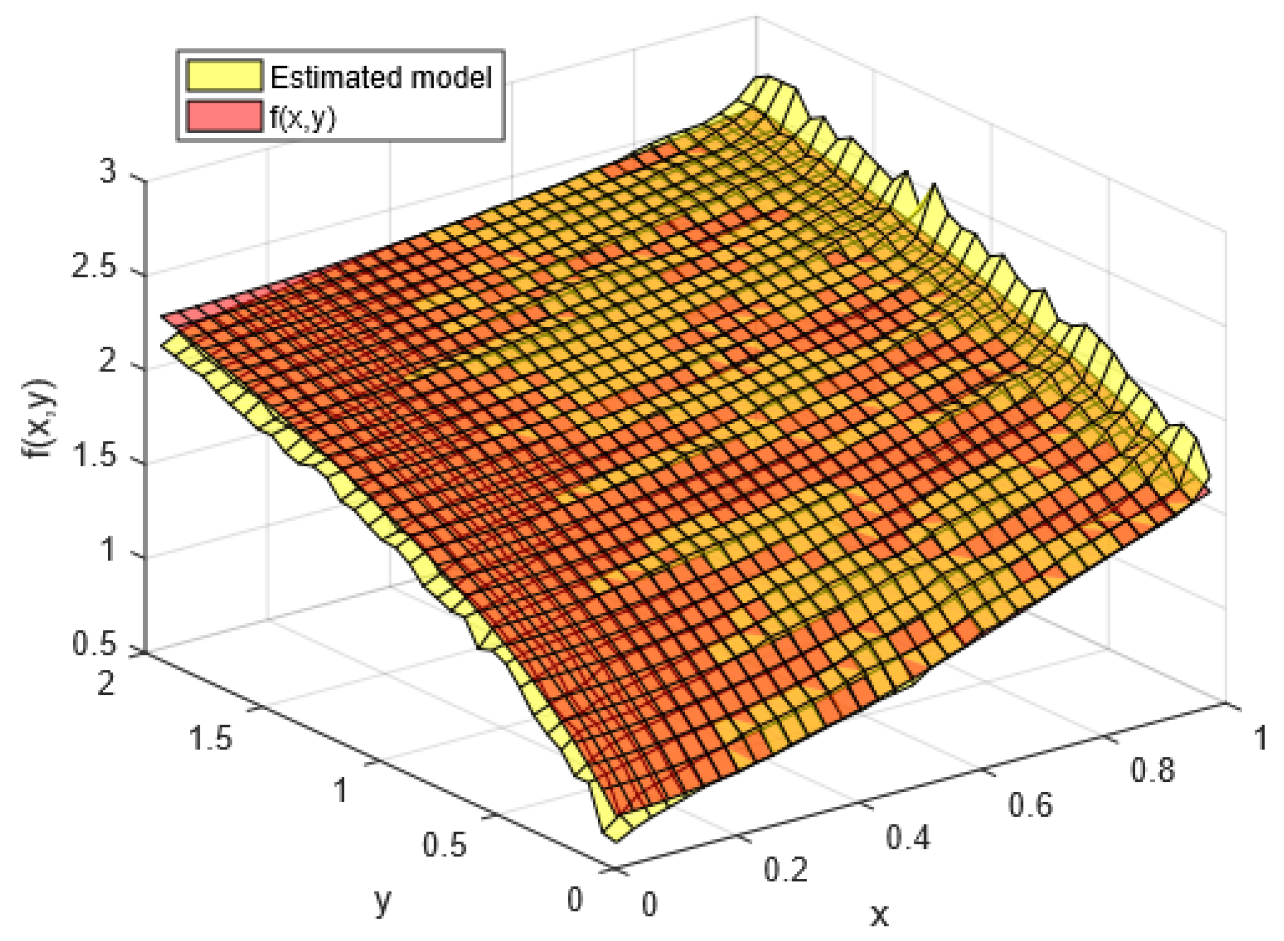
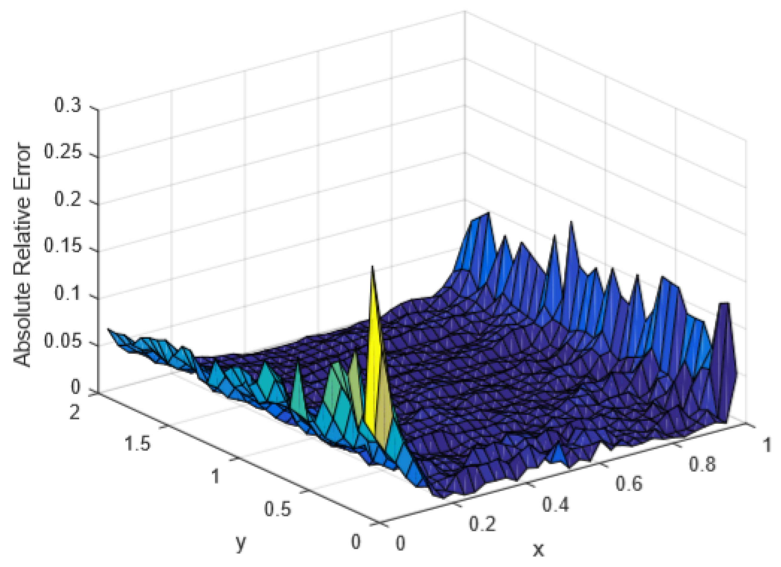
3.1.1. Synthetic Dataset 1: Know Mathematical Function

In this experiment, three variables subject to modeling, namely x, y and z, were generated as follows: the variable x takes random values uniformly distributed within the interval [ 0 , 1 ] , the variable y takes random values uniformly distributed within the interval [ 0 , 2 ] , and the variable z is computed according to the known non-linear function u ( x , y ) = def log ( 3 x 2 + 4 y + 2 ) , corrupted by an additive zero-mean Gaussian random noise ε , with standard deviation σ ε = 0.1 , namely z = u ( x , y ) + ε . A total of 10,000 samples were generated.
The Figure 9 and Figure 10 show the results obtained by the modeling algorithm recalled in the Section 2.1. In particular, the Figure 9 shows the estimated model superimposed with the true function, while Figure 10 shows the absolute (point-wise) relative error, computed by the formula
e rel x , y = def f x , y z ^ x , y f x , y ,
where z ^ ( x , y ) represents the value of the inferred model corresponding to the values ( x , y ) of the independent variables. This error formula measures the absolute value of the deviation between the actual model and the inferred model at any discrete location, normalized by the absolute value of the model at the same location, in order to get a relative (percentage-like) deviation.
The numerical results displayed in Figure 9 confirm that the algorithm recalled in the Section 2.1 is able to infer a faithful model of the data and the numerical errors displayed in Figure 10 confirm that the relative errors are far below 0.05 at the middle of the ( x , y ) -domain (that is, the absolute error is less than 5 % relatively to the maximum absolute value of the model).
The Figure 11 and Figure 12 show the results obtained, on the same dataset, by the modeling algorithm explained in the Section 2.2. In particular, the Figure 11 shows the estimated model superimposed with the true function for the ease of comparison, while Figure 12 shows the relative error, as computed by the Formula (14).
The results displayed in Figure 11 show that the improved algorithm recalled in the Section 2.2 is able to infer a faithful model of the data and the the numerical errors displayed in Figure 12 confirm that, even in this case, the relative errors are far below 0.05 at the middle of the ( x , y ) -domain.
In order to perform a comparison of the previous results that take into account the modeling performance over the whole domain, it is convenient to define a numerical index that summarizes local estimation errors. On the basis of the values of the absolute point-wise relative errors, the following average relative error index was defined:
e ¯ rel = def 1 S y S x i = 1 S y j = 1 S x e rel i , j .
Applying this formula to the results obtained by both algorithms, it is obtained that the average error corresponding to the algorithm recalled in the Section 2.1 is e ¯ rel = 0.0201 , while the average error corresponding to the refined algorithm explained in the Section 2.2 is e ¯ rel = 0.0188 . Therefore, from the results of this experiment, it may be concluded that the refined version of the algorithm yields a more precise estimation of the model than the previous algorithm that it originated from.

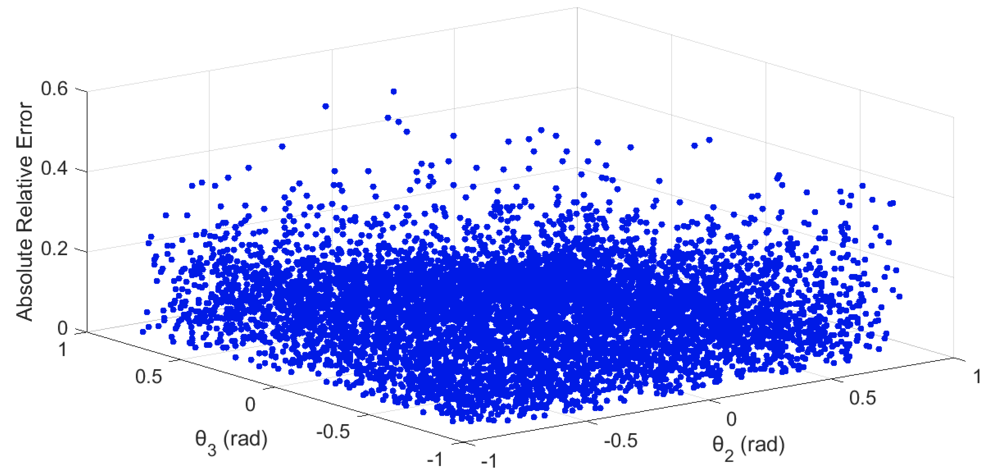
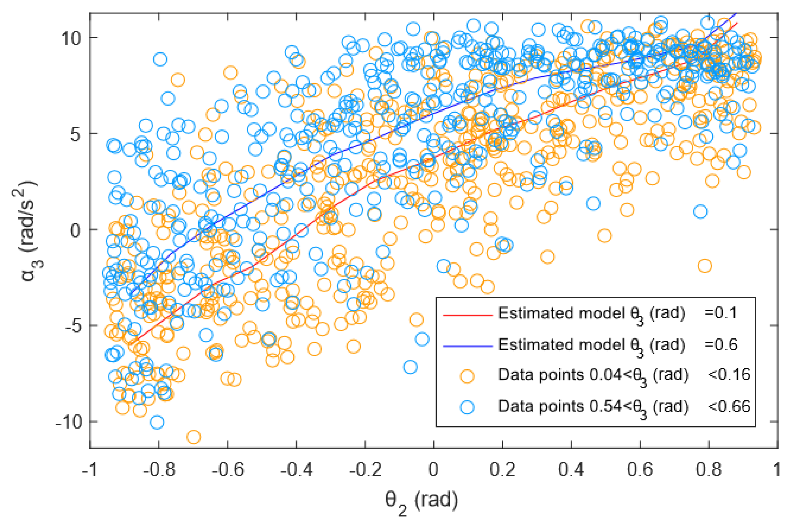
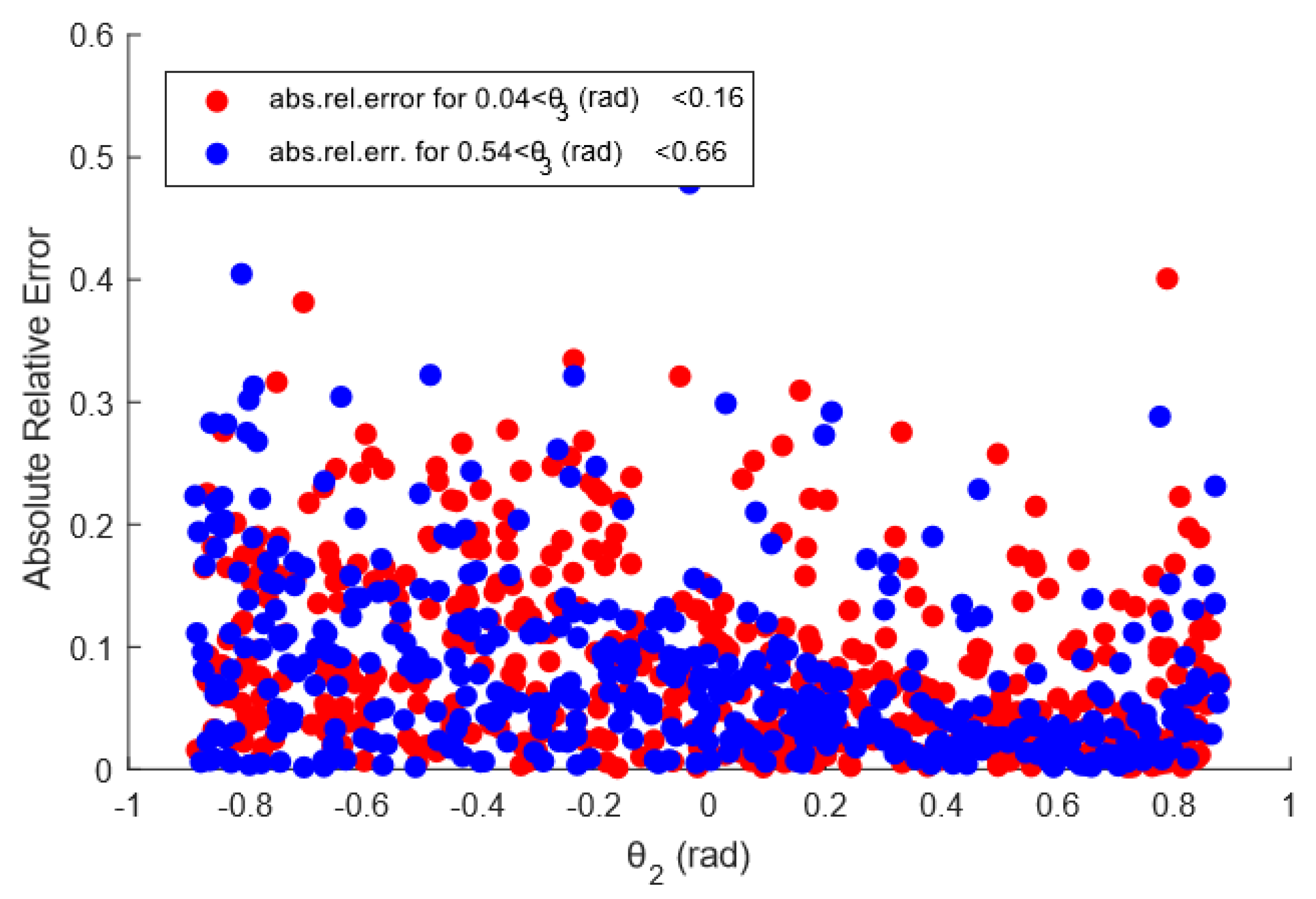
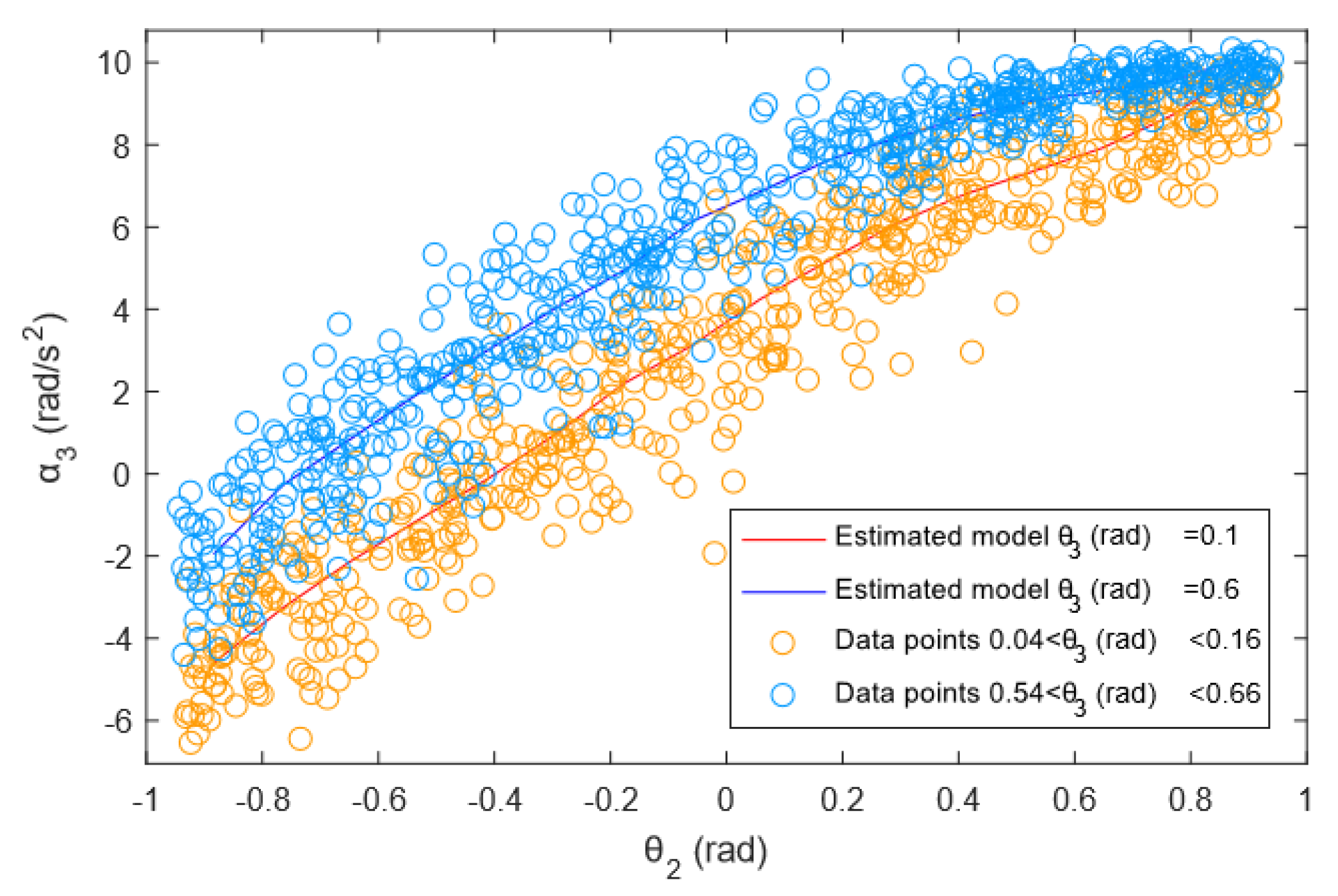
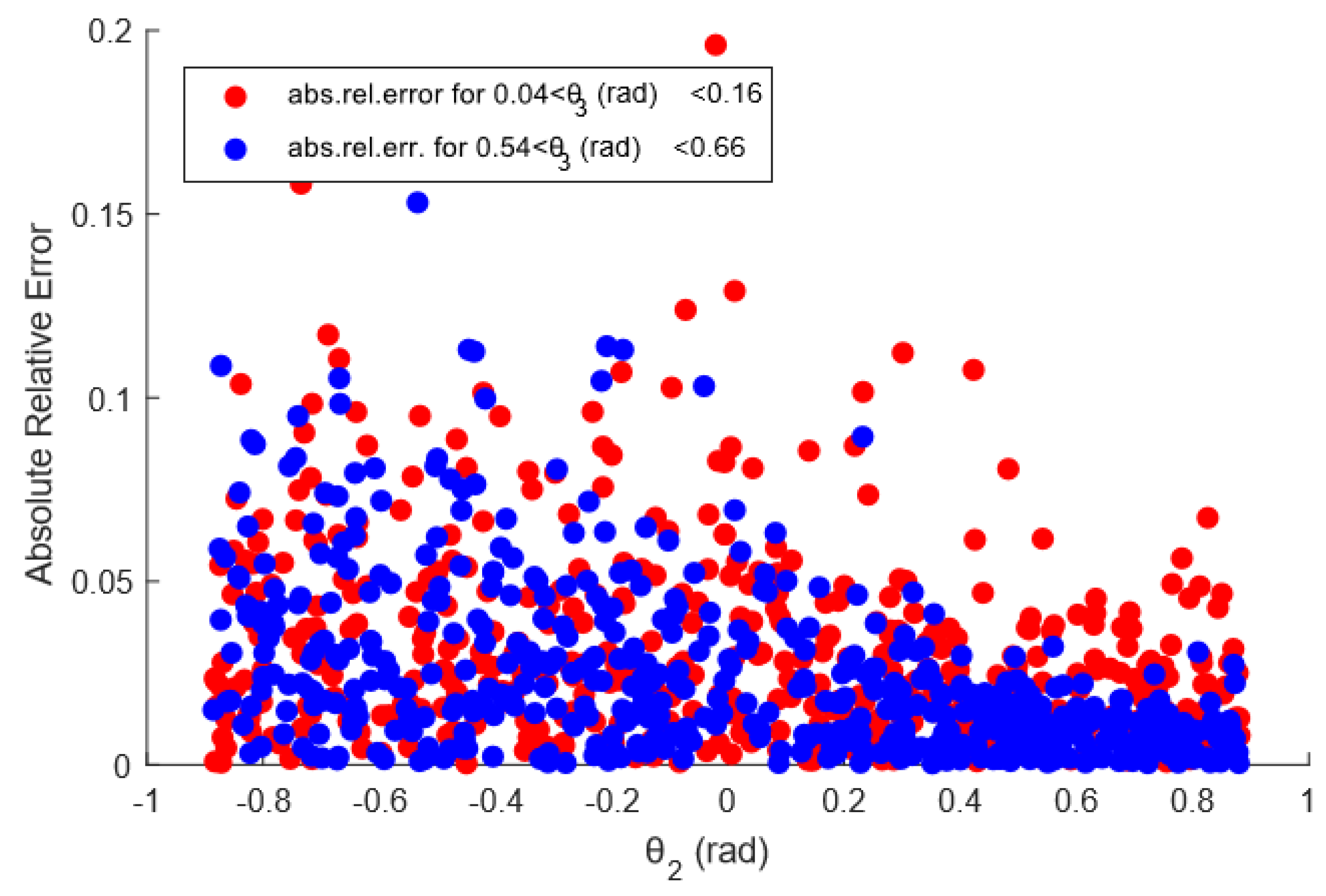
3.1.2. Synthetic Datasets 2—PUMA Robot

The “PUMA robot” ensemble counts a total of four distinct datasets, where each variable represents a mechanical quantity, such as the angular position, the angular speed, the mechanical torque and the angular acceleration of different joints in a mathematical model of a robotic arm [39].
Only two of these datasets may be modeled by means of the algorithms explained in the Section 2 since they are explained by monotonic dependencies. These datasets count a number of 8192 data-records. We applied the algorithms to the modeling of the angular acceleration α 3 of the third joint as a function of the angular positions of the second and of the third joint, namely θ 2 , θ 3 , with α 3 [ 12 , 12 ] rad s 2 , θ 2 and θ 3 [ 1 , 1 ] rad .
The Figure 13 and Figure 14 show the results obtained, on the first dataset, by the modeling algorithm explained in the Section 2.2. In particular, the Figure 13 shows the estimated model superimposed with the data, while Figure 14 shows the relative error, computed by an expression similar to (14), where the unknown function f has been replaced with the available data, namely:
e rel x s , y s = def z s z ^ x s , y s z s ,
where ( x s , y s , z s ) represent the triples of the available data and z ^ ( x s , y s ) represents the value returned by the inferred model corresponding to the values ( x s , y s ) of the independent variables.
The numerical results displayed in Figure 13 show a feature of statistical modeling in the presence of largely noisy data, namely, the ability to infer a model whose representative surface locates amid the data points, without necessarily touching the data themselves. The Figure 14 shows that the relative error is uniformly distributed within the domain and, in most of the points, it is far less than 0.2 .
In addition, the Figure 15 shows two slices of the model obtained for two different values of the value θ 3 taken as a constant in a given range, while Figure 16 illustrates the value of the relative error between the slices of the model at constant θ 3 in a given range and the corresponding data in the datasets.
As it may readily be appreciated from Figure 16, in spite of the relatively large variance in the data, the inferred model looks quite faithful, with a relative error that, for most of the data-points, is less than 0.2 .
The Figure 17 and Figure 18 show the results obtained, on the second “PUMA robot” dataset, by the modeling algorithm explained in the Section 2.2. In particular, the Figure 17 shows the estimated model superimposed with the data, while Figure 18 shows the relative error.
In comparison with the first “PUMA robot” dataset, it is immediately appreciated how these data appear far less noisy, hence the non-linear model built through the algorithm explained in the Section 2.2 is more effective in representing the data. In fact, as can be directly observed from the error scatter plot of Figure 18, the relative error for most of the points is less than 0.05 .
The Figure 19 shows two slices of the model obtained for two different values of the value θ 3 taken as a constant in a given range, while Figure 20 illustrates the value of the relative error between the slices of the model at constant θ 3 in a given range and the corresponding data in the datasets.
As opposed to the first dataset, the second datasets contains data that appear far less noisy, therefore, the model obtained for the second dataset looks more faithful and adherent to the data. In fact, from Figure 16 it can be readily appreciated how, over the considered data-slices, the relative error is below 5 % for most of the data points depicted in the data-slice plot.

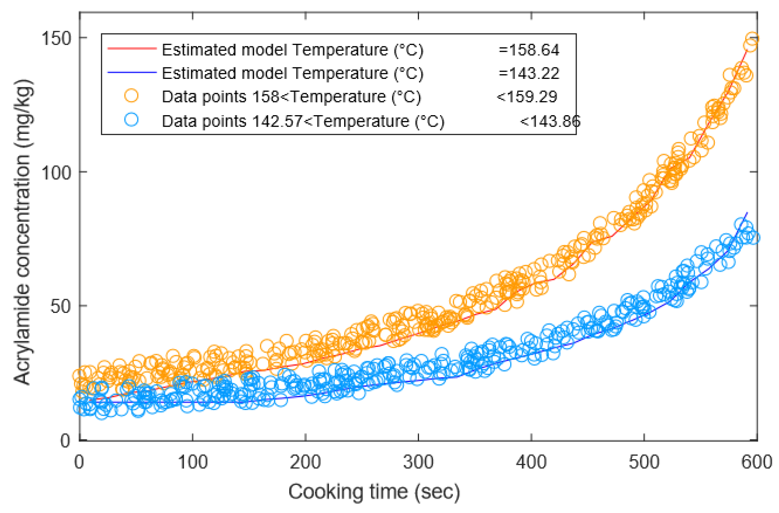
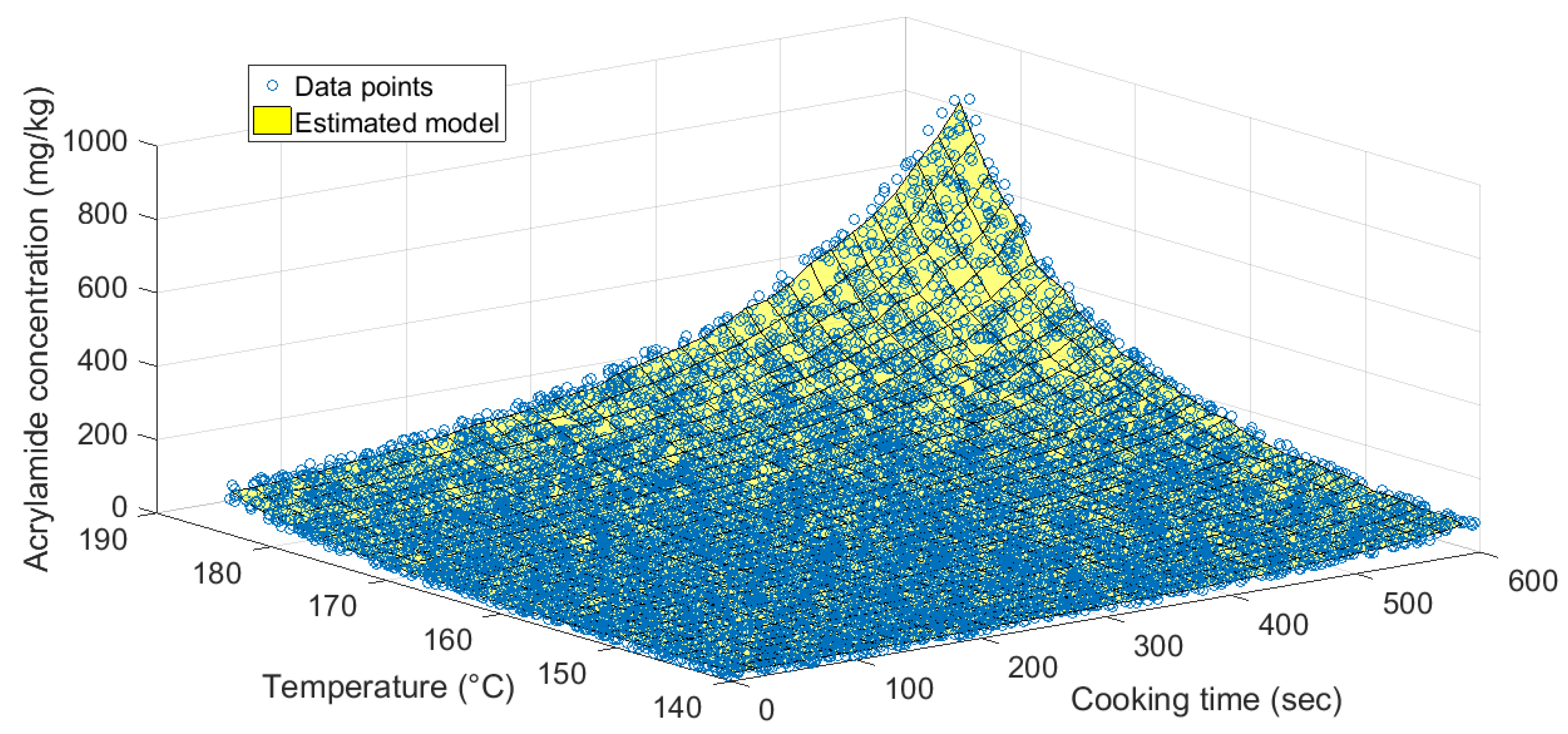
3.1.3. Synthetic Dataset 3—Acrylamide Formation in French Fries

This dataset concerns the formation of a cancerogenic chemical, known as acrylamide, during the process of cooking ‘French fries’, as investigated upon in the food toxicology study [29]. This dataset consists of three independent variables, namely cooking time t and cooking temperature T, which are the independent variables, and acrylamide concentration C A . This dataset consists of 10,000 triples, with values ranging in [ 0 , 600 ] s, [ 140 , 185 ] C and [ 0 , 810 ] mg kg , respectively.
The Figure 21 shows the results obtained by the modeling algorithm explained in the Section 2.2. In particular, the Figure 21 shows the estimated model superimposed with the data.
As it can be observed from Figure 21, the concentration of acrylamide formed during the process of cooking raw fries grows both with the cooking time and with the cooking temperature, namely:
C A t t , T > 0 and C A T t , T > 0 .
Also, the data scatter plot in Figure 21 shows that this dataset is not affected by noise, therefore the model built through the algorithm explained in the Section 2.2 is faithful.
The Figure 22 shows two slices of the model obtained for two different values of the cooking temperature taken as a constant in a given range.
From the above figures, it is immediate to conclude that the modeling process, with these well-tamed data, is completely faithful to the data.

3.1.4. Synthetic Dataset 4—Pollen Grains

This is a synthetic dataset used, e.g., in [40,41], which contains five variables that describe physical as well as geometric features of 3846 pollen grains (namely, geometric dimensions along three orthogonal axes, weight and mass density) and is publicly available for download at [42].
In this experiment, a geometric dimension referred to as ridge (assigned to the variable z) was taken as dependent variable to be modeled as a function of two independent physical variables (weight, assigned to the variable x, and density, assigned to the variable y). In this dataset, these three variables are dimensionless, are expressed in arbitrary scales and range in [ 30 , 17 ] , [ 40 , 28 ] and [ 7 , 14 ] , respectively (for more details on how these data have been generated from a physical model and pre-processed, readers might consult [42]).
By a pre-screening of the values in the dataset, it emerged that the dependent variable z shows a decreasing trend with respect to the independent variable x, namely z x x , y < 0 , ( x , y ) . In this case, before running the modeling procedure, the sign of the z-variable was reversed so as to recover a monotonically increasing trend. The sign of the obtained model was then reversed in order to draw figures which are consistent with the data.
The Figure 23 and Figure 24 show the results obtained by the proposed modeling algorithm. In particular, the Figure 23 shows the estimated model superimposed with the data, while Figure 24 shows the values of the absolute point-wise relative error over the data-domain.
As opposed to the first three datasets, the ‘Pollen grain’ dataset is not defined on a rectangular domain, as the ( x , y ) -values appear to belong to an irregular domain. This fact poses a challenge to the modeling algorithm that is based on a regular subdivision into a uniform mesh of the domain. At the center of the domain the model explains the data faithfully, while at the periphery of the domain the model essentially provides a linear prediction, due to lack of information in the dataset.
The Figure 25 shows two slices of the model obtained for two different values of the mass density taken as a constant in a given range, while Figure 26 illustrates the value of the relative error between the slices of the model at constant mass density in a given range and the corresponding data in the datasets.
In this experiment, the results obtained by running the proposed modeling technique on the two data-slices are in excellent agreement with the data, in spite of the irregular shape of the data domain, since the relative error in most of the points is less than 10 % .

3.2. Experiments on Natural Datasets

The present section illustrates and discusses the results of several non-linear trivariate regression tests performed on five natural datasets. In contrast to synthetic datasets, the natural datasets considered in the following sections contain a limited number of data-records, due to the fact that obtaining good quality data might result in a costly process.
All the datasets contain more than three variables, therefore, each dataset has been pre-screened in order to extract a dependent variable to model as a function of two independent variables. Moreover, due to the nature of the physical quantities taken into account, the corresponding variables might present values spanning several orders of magnitude or too concentrated around zero: in these cases, a non-linear invertible pre-processing has been put into effect in order to make their values more evenly distributed; each transformation has been then reversed after modeling.
Variables pre-selection has been performed on the basis of pair-wise correlation analysis. The coefficient of correlation between two variables is defined as
ρ x , y = def σ x , y σ x σ y ,
where σ x and σ y denote (empirical) standard deviations, while σ x , y denotes an empirical covariance coefficient defined as
σ x , y = 1 S s = 1 S ( x s x ¯ ) ( y s y ¯ ) .
On the basis of these definitions, it holds that 1 ρ x , y 1 , namely, the smaller is the statistical correlation between two variable, the closer the coefficient of correlation is to zero. For each dataset, we selected those three variables which showed a correlation coefficient closer to 1.

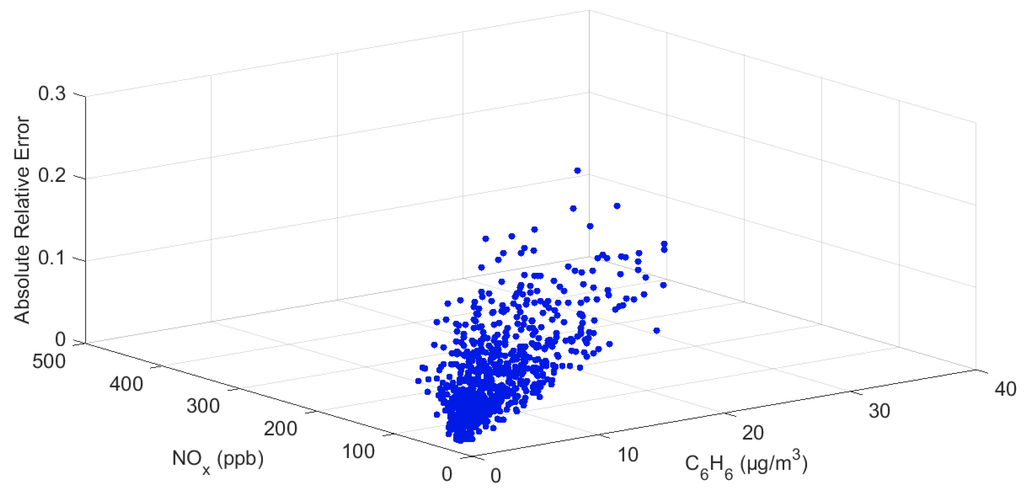
3.2.1. Natural Dataset 1—Air Quality

This dataset contains the concentration of five air pollutants, recorded through chemical sensors collocated in a significantly polluted geographical area (within an Italian region), during the time-frame of March 2004 to February 2005 [30]. This dataset consists of 827 records. Among the five chemical concentrations, the concentration of carbon dioxide (CO 2 ) in air was chosen as dependent variable to be modeled as a function of benzene (C 6 H 6 ) concentration and mono-nitrogen oxides (NO X ) concentration as independent variables. These three variables range in [ 0 , 40 ] μ g m 3 , [ 0 , 500 ] ppb and [ 0 , 9 ] mg m 3 , respectively. (The acronym ‘ppb’ denotes ‘parts per billion’, a measure of concentration; 1 ppb is equal to 1 microgram per liter.)
The Figure 27 and Figure 28 show the results obtained by the proposed modeling algorithm. In particular, the Figure 27 shows the estimated model superimposed with the data, while Figure 28 shows the values of the absolute point-wise relative modeling error.
As it is readily seen from Figure 27 and Figure 28, this dataset is not defined on a rectangular domain but rather on an irregular domain. This is often the case for natural datasets, as some combinations of the instances of the x-variable or the y-variable are not plausible. As it can be observed from Figure 27, the modeling algorithm is able to infer values even in those areas of the domain where there are no experimental data available by linear interpolation. The Figure 28 shows that, for most data-points, the relative error is less than 10 % .

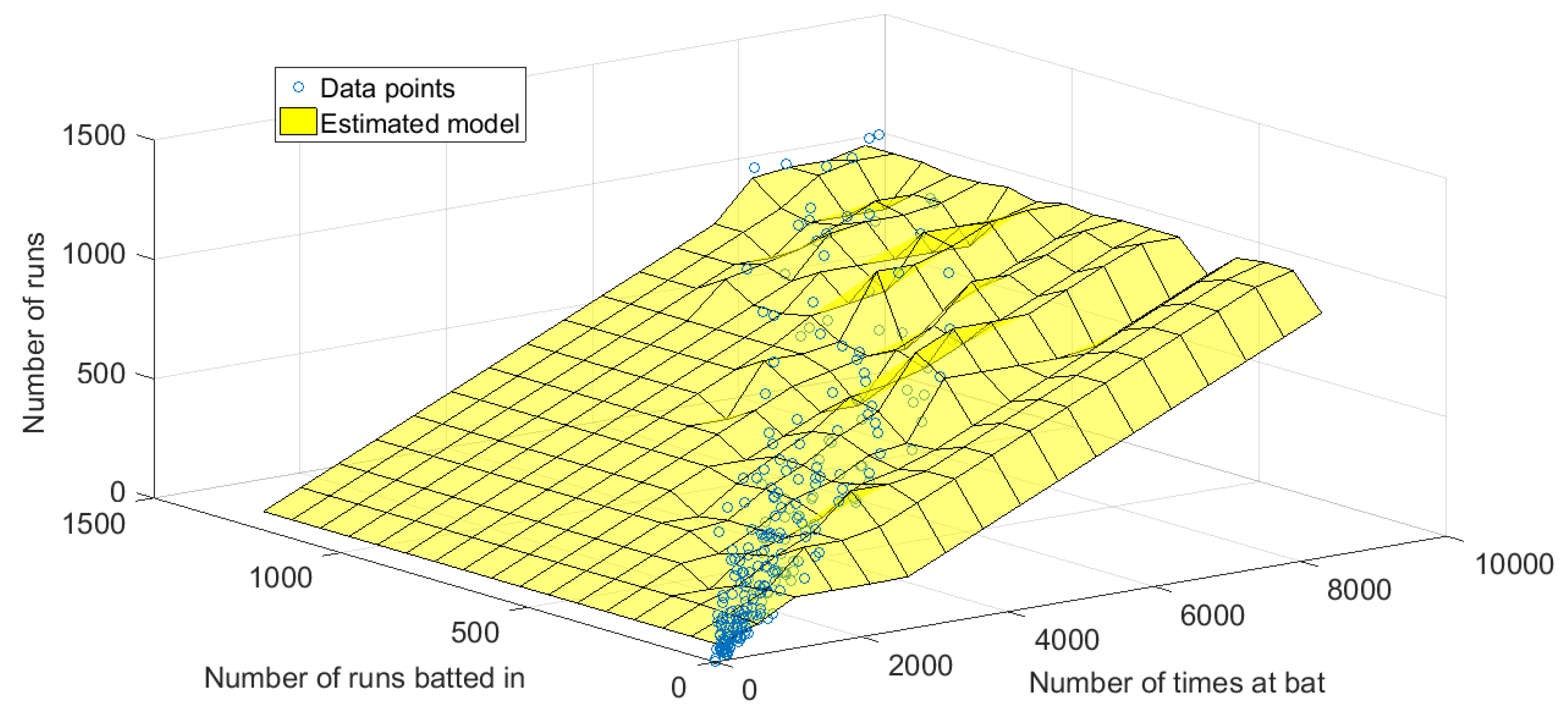
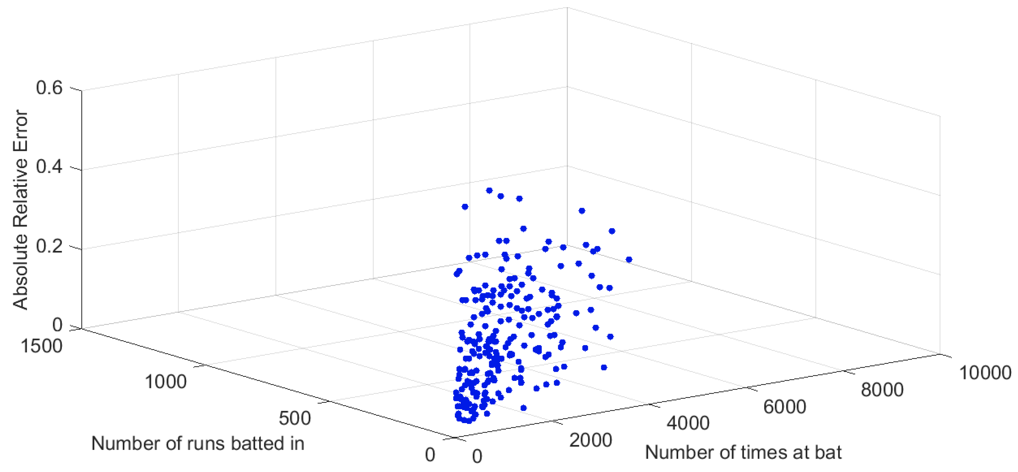
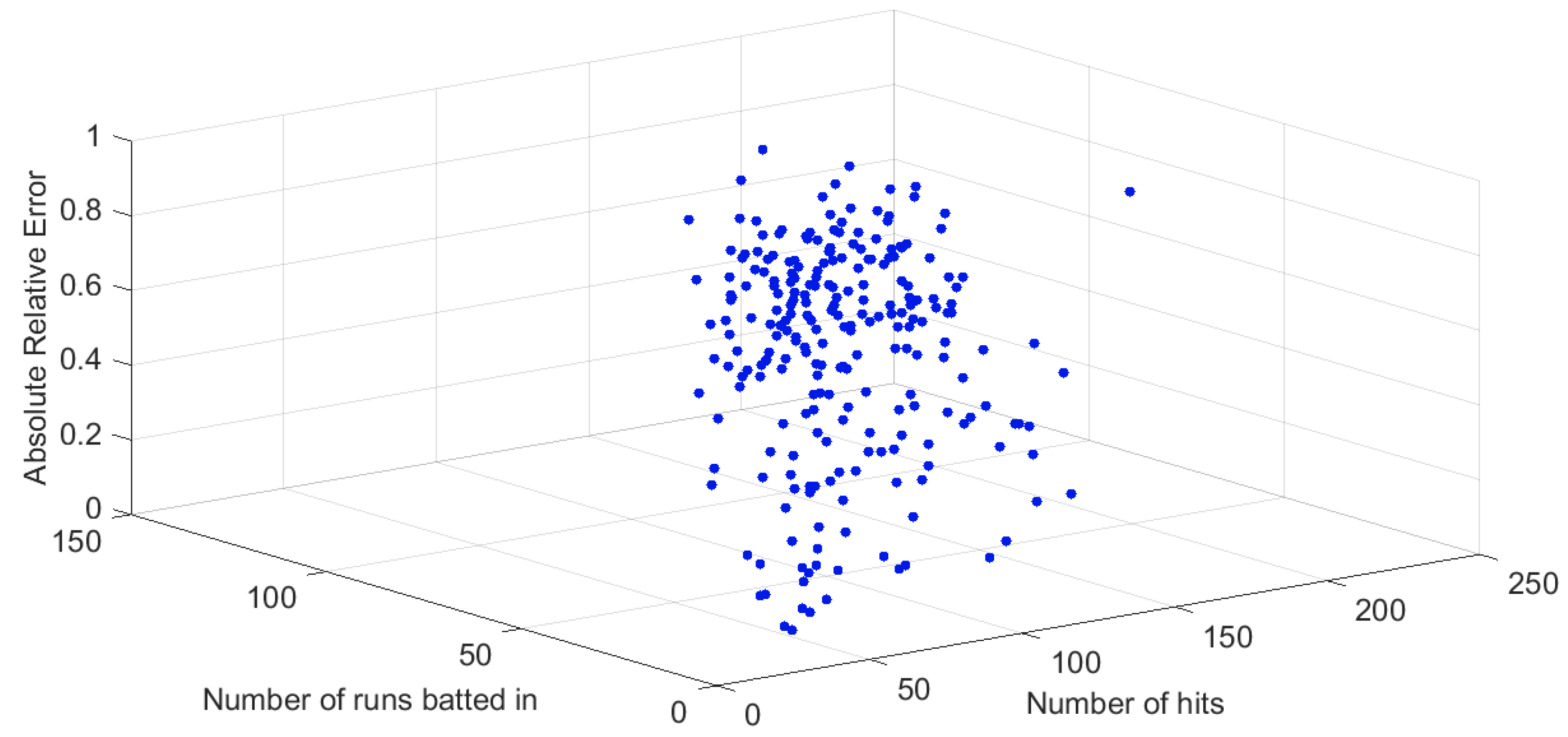
3.2.2. Natural Dataset 2—Baseball Players Salary

This dataset consists of entries from official statistics about 260 Major League Baseball (MLB) players of the years 1986–1987 [43] and contains a total of 24 variables. On the basis of a correlation pre-screening of these variable, we considered two different combinations of three variables, namely:
  • Combination 1: Modeling ‘Number of runs’ (Runs during player’s career) as a function of ‘Number of times at bat’ (AB during player’s career) and ‘Number of runs batted in’ (RBI during player’s career). These three variables range in [ 0 , 1200 ] , [ 0 , 9000 ] and [ 0 , 1400 ] , respectively.
  • Combination 2: Modeling ‘Annual salary in 1987’ as a function of ‘Number of runs batted in’ (RBI in 1986) and ‘Number of hits’ (H in 1986). These three variables range in [ 675 , 000 , 2 , 460 , 000 ] $, [ 15 , 125 ] and [ 40 , 240 ] , respectively.
The rationale of this double choice is that, given a dataset to model, the performance of the algorithm might change according to which variables are chosen for modeling purposes.
The Figure 29 and Figure 30 show the results obtained by the proposed modeling algorithm on the Combination 1. In particular, the Figure 29 shows the estimated model superimposed with the data, while Figure 30 shows the values of the absolute point-wise relative error.
From these results it may be observed how, in spite of the scarcity—in terms of quantity—of available data-records, for the Combination 1 of variables the inferred model results quite faithful to the data. In fact, as it may be observed directly from Figure 29, the dependent variable takes a perceivable increasing trend which is captured by the model as well.
Before running the modeling algorithm on the Combination 2 of variables, because of the large range of values taken by the dependent variable z (Annual salary in 1987), we performed a non-linear pre-processing of the dependent variable described by z ˜ = def log ( z ) , yielding a narrower interval of values. Upon running the modeling algorithm, we reversed the pre-processing transformation to get back to natural values.
The Figure 31 and Figure 32 show the results obtained by the proposed modeling algorithm on the Combination 2. In particular, the Figure 31 shows the estimated model superimposed with the data, while Figure 32 shows the values of the absolute point-wise relative modeling error.
In this experiment, one may observe how the model does not appear sufficiently faithful to the data for the Combination 2 of variables. In fact, from Figure 32, one may observe how several absolute relative error values are close to the unity. This experiment show that, although the independent variables show a high correlation to the dependent variable, it is not always possible to build a model that explains their relationship based on a few observations, if their relationship is exceedingly complex.

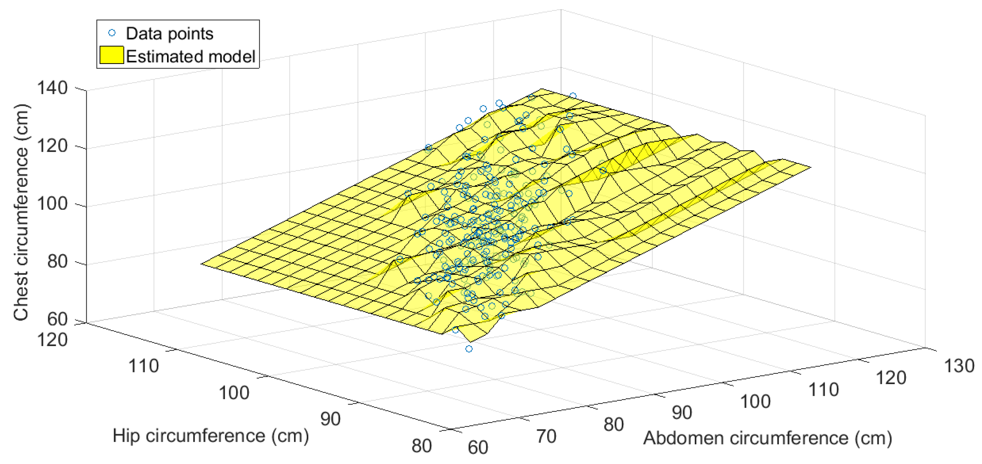
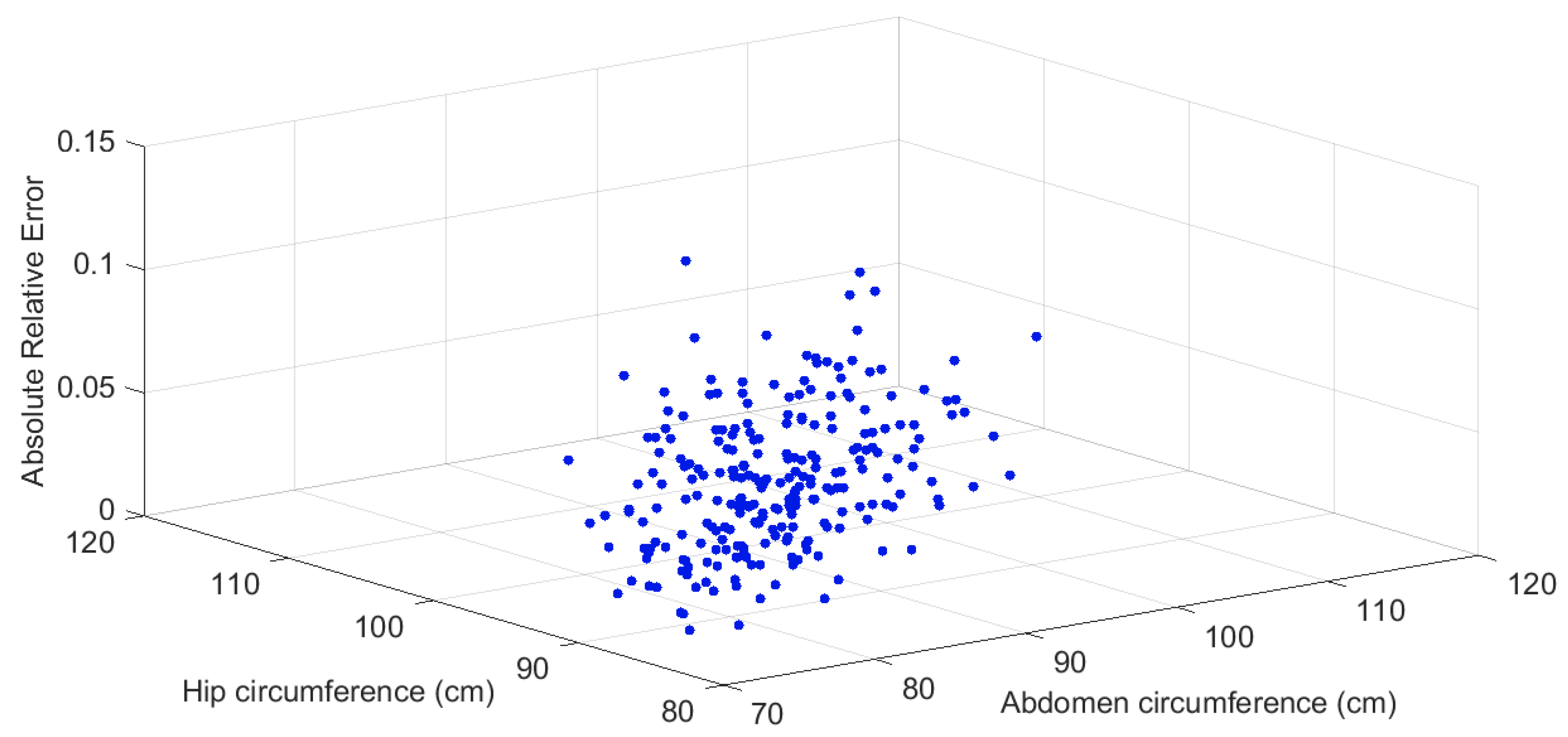
3.2.3. Natural Dataset 3—Body Fat

This dataset contains data records about different body sizes along with the age, the height, the weight and the percentage of body fat of 252 individuals [44]. In this experiment, the circumference of the pectoral area has been selected to be the dependent variable to model as a function of the circumference of the abdomen and of the circumference at the hip. Such variables range in [ 70 , 116 ] cm, [ 80 , 130 ] cm and [ 91 , 120 ] cm, respectively.
The Figure 33 and Figure 34 show the results obtained by the proposed modeling algorithm. In particular, the Figure 33 shows the estimated model superimposed with the data, while Figure 34 shows the values of the absolute point-wise relative error.
The results obtained by running the modeling algorithm show particularly low relative errors compared to previous datasets. In fact, most of the relatiove modeling errors appearing in Figure 34 take a value less than 10%. The Figure 33 shows that the algorithm is able to extend the model around the natural domain of the data, hence affording the prediction of the ‘Chest circumference’ value in terms of joint instances of the ‘Hip circumference’ and of the ‘Abdomen circumference’ values that are less frequently observed. The inferred model appears reliable as the general trend appears in good agreement with the data.

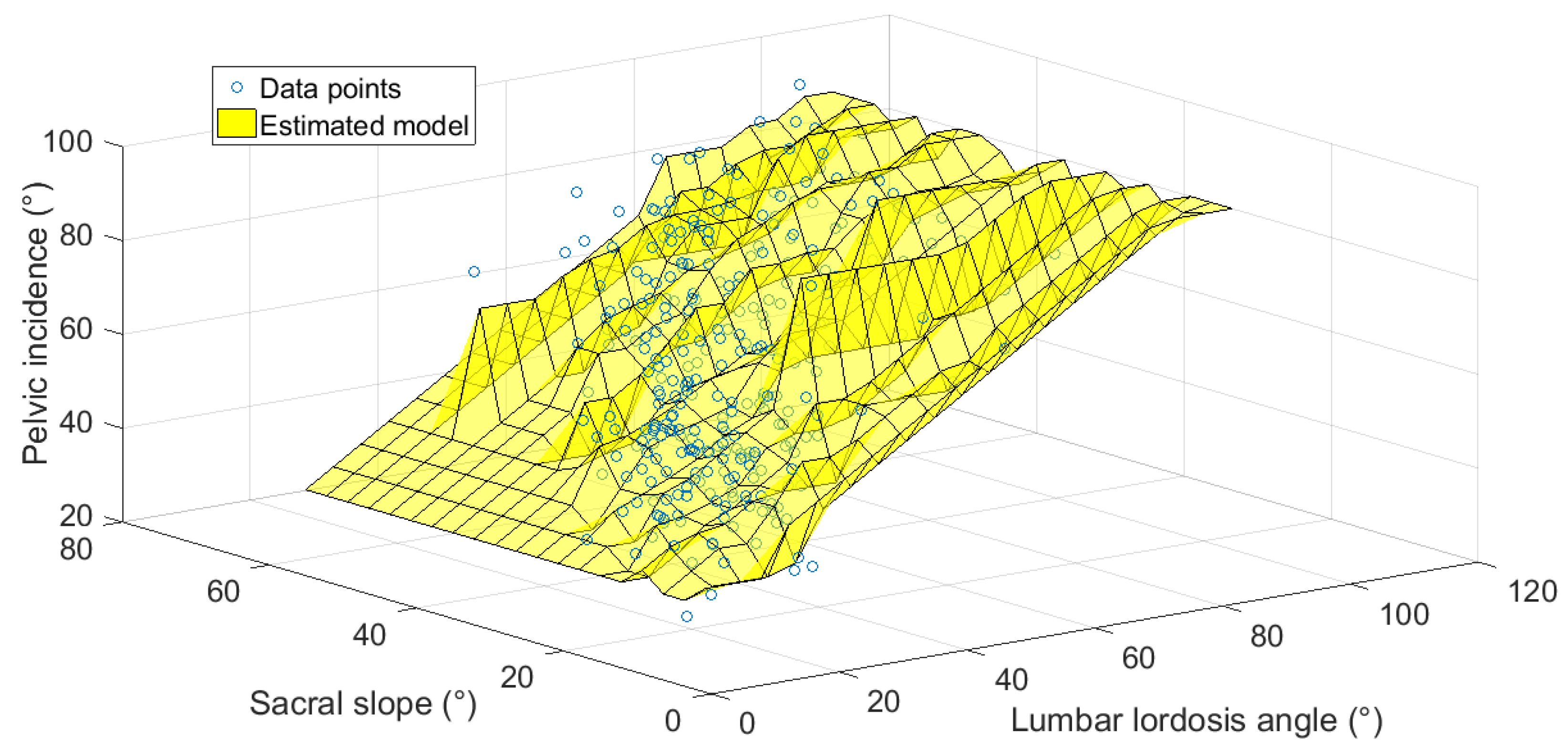
3.2.4. Natural Dataset 4—Vertebral Column

This data-dataset contains numerical attributes about the vertebral column of 304 individuals [45]. The modeling problem takes the pelvic incidence index as dependent variable to be modeled as a function of the sacral slope and of the lumbar lordosis angle taken as independent variables. Their values range in the intervals [ 20 , 100 ] deg, [ 20 , 80 ] deg and [ 20 , 110 ] deg, respectively.
The Figure 35 and Figure 36 show the results obtained by the proposed modeling algorithm. In particular, the Figure 35 shows the estimated model superimposed with the data, while Figure 36 shows the values of the absolute point-wise relative modeling error.
From Figure 36 is it easy to recognize that there are only two points where the relative error is larger than 40% that, most likely, represent outliers. Therefore, even in this experiment, the statistical modeling process looks successful and the built trivariate model look faithful to the dataset.

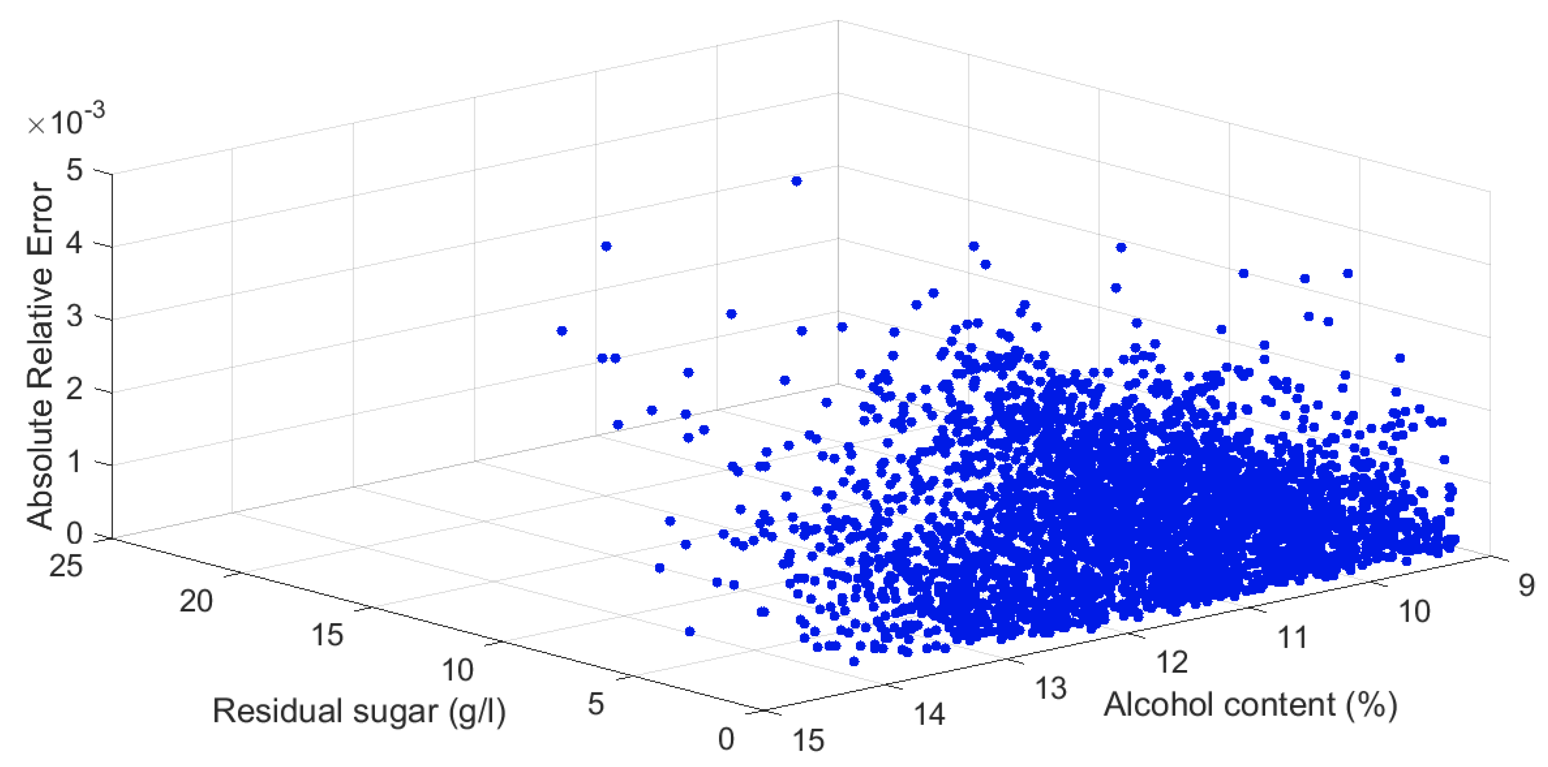
3.2.5. Natural Dataset 5—White Wine Characteristics

This dataset contains records about 10 chemical properties of 4,577 different samples of white wine [46]. The modeling process was performed by taking the volumetric density as dependent variable to be modeled as a function of the alcoholic content and of the residual sugar level. Such values range in the intervals [ 0.986 , 1.001 ] g mL , [ 9.0 , 14.2 ] % and [ 1 , 21 ] g L , respectively.
The Figure 37 and Figure 38 show the results obtained by the proposed modeling algorithm. In particular, the Figure 37 shows the estimated model superimposed with the data, while Figure 38 shows the values of the absolute point-wise relative error.
The Figure 37 shows that the algorithm is able to extend the model far beyond the natural domain of the data, hence affording the prediction of the ‘Density’ value in terms of joint instances of the ‘Residual sugar’ and of the ‘Alcohol content’ values that are less frequently observed. The inferred model appears reliable as the general trend appear in good agreement with the available data. From Figure 38, it can be noticed how the magnitude order of the relative errors is about 10 3 .
The Figure 39 shows two slices of the model obtained for two different values of the alcohol concentration taken as a constant in a predefined range, while Figure 40 illustrates the value of the relative error between the slices of the model at constant alcohol concentration in a given range and the corresponding data in the datasets. From these figures, it can be readily concluded that, in this experiment, the results achieved by the proposed statistical modeling algorithm are excellent.

4. Conclusions

The present paper discusses an improved numerical algorithm to perform statistical isotonic trivariate modeling. The distinguishing features of the presented statistical modeling technique may be summarized as follows:
  • The proposed algorithm does not make direct use of the data samples but rather extracts collective information from the data and represent such information by second-order joint probability functions. As a consequence, the model does not fit the data samples (which may be unreliable due to measurement errors or unknown hidden/nuisance variables) but rather captures the overall structure of the underlying physical system.
  • The principle informing the discussed modeling procedure is drawn from a probability conservation law, which differentiates the proposed modeling concept from the classical deterministic linear/non-linear fitting schemes. The underlying probability conservation law holds true irrespective of the shape of the involved probability density functions and model, provided that continuity and monotonicity hold.
  • The proposed procedure does not make any assumption on the shape of the model, except for continuity and monotonicity. As a result, the model is unrestricted and there is no need to choose any functional dependency beforehand, which differentiates the proposed modeling from the parametric/maximum-likelihood estimation methods.
  • The involved quantities, namely, the probability density functions and the inferred model, are represented by simple numerical tables. The probability density functions are estimated by constructing occurrence histograms and the associated marginal cumulative distribution functions are estimated by cumulative sums. The model is estimated by proximity search within the tables, which only require basic mathematical operations. The resulting procedure is computationally light and very fast to execute.
The presented numerical experiments confirmed that the inferred statistical model is in good agreement with the data at the center of the grid, while a larger relative error is observed in the peripheral part of the domain.
An interesting feature of the proposed modeling algorithm is that, while being based on joint probability estimation, its capability of building a model faithful to the data is retained even when the size of the datasets is limited. In fact, the results of the numerical experiments shown in the Section 3 confirm that the algorithm is able to infer meaningful models even for limited-size datasets.
A further interesting feature that emerged, in particular, from the experiments performed on the natural datasets, is the ability to deal with datasets that do not cover the ( x , y ) -domain uniformly but are rather concentrated on irregular areas of the x-y plane, due to the fact that some values of the x-variable and of the y-variable are not jointly physically plausible or are less frequently encountered. This affords the estimation of the values of the dependent variable in terms of joint instances of the two independent variables that are less frequent. This fact affords testing hypotheses on the behavior of an actual physical system beyond the domain of its direct observation.
The main drawback of the proposed non-linear trivariate modeling algorithm is that it can cope only with monotonic dependencies among the two independent variable and the dependent variable. We are currently working toward an extension of this algorithm to modeling non-monotonic dependencies, hence toward non-istonic non-linear modeling.

Author Contributions

Conceptualization, S.F.; Software, A.V.; Writing—original draft, A.V.; Writing—review & editing, S.F.

Funding

This research received no external funding.

Acknowledgments

The authors would like to thank the anonymous reviewers for the careful proofreading of the paper and for suggesting several useful changes that contributed to improving the quality of the presentation.

Conflicts of Interest

The authors declare no conflict of interest.

References

  1. Kroese, D.P.; Chan, J.C.C. Statistical Modeling and Computation; Springer: Berlin, Germany, 2014. [Google Scholar]
  2. Carrara, P.; Altamura, E.; D’Angelo, F.; Mavelli, F.; Stano, P. Measurement and numerical modeling of cell-free protein synthesis: combinatorial block-variants of the PURE system. Data 2018, 3, 41. [Google Scholar] [CrossRef]
  3. Chu, P.C. World ocean isopycnal level absolute geostrophic velocity (WOIL-V) inverted from GDEM with the P-Vector method. Data 2018, 3, 1. [Google Scholar] [CrossRef]
  4. Hoseinie, S.H.; Al-Chalabi, H.; Ghodrati, B. Comparison between Simulation and Analytical Methods in Reliability Data Analysis: A Case Study on Face Drilling Rigs. Data 2018, 3, 12. [Google Scholar] [CrossRef]
  5. Reed, F.J.; Gaughan, A.E.; Stevens, F.R.; Yetman, G.; Sorichetta, A.; Tatem, A.J. Gridded population maps informed by different built settlement products. Data 2018, 3, 33. [Google Scholar] [CrossRef]
  6. Stein, M.; Janetzko, H.; Seebacher, D.; Jäger, A.; Nagel, M.; Hölsch, J.; Kosub, S.; Schreck, T.; Keim, D.A.; Grossniklaus, M. How to make sense of team sport data: From acquisition to data modeling and research aspects. Data 2017, 2, 2. [Google Scholar] [CrossRef]
  7. Torbati, M.E.; Mitreva, M.; Gopalakrishnan, V. Application of taxonomic modeling to microbiota data mining for detection of helminth infection in global populations. Data 2016, 1, 19. [Google Scholar] [CrossRef] [PubMed]
  8. Vakanski, A.; Jun, H.-P.; Paul, D.; Baker, R. A data set of human body movements for physical rehabilitation exercises. Data 2018, 3, 2. [Google Scholar] [CrossRef]
  9. Vorster, A.G.; Woodward, B.D.; West, A.M.; Young, N.E.; Sturtevant, R.G.; Mayer, T.J.; Girma, R.K.; Evangelista, P.H. Tamarisk and Russian olive occurrence and absence dataset collected in select tributaries of the Colorado River for 2017. Data 2018, 3, 42. [Google Scholar] [CrossRef]
  10. Archontoulis, S.; Miguez, F. Nonlinear regression models and applications in agricultural research. Agron. J. 2015, 107, 786–798. [Google Scholar] [CrossRef]
  11. Bates, D.; Watts, D. Nonlinear Regression Analysis and Its Applications, 2nd ed.; John Wiley & Sons: Hoboken, NJ, USA, 2007. [Google Scholar]
  12. He, X.; Ng, P.; Portnoy, S. Bivariate quantile smoothing splines. J. R. Stat. Soc. 1998, 60, 537–550. [Google Scholar] [CrossRef] [Green Version]
  13. Kravtsov, S.; Kondrashov, D.; Ghil, M. Multilevel regression modeling of nonlinear processes: Derivation and applications to climatic variability. J. Clim. 2005, 18, 4404–4424. [Google Scholar] [CrossRef]
  14. Payandeh, B. Some applications of nonlinear regression models in forestry research. For. Chron. 1983, 59, 244–248. [Google Scholar] [CrossRef]
  15. Rusov, J.; Misita, M.; Milanovic, D.D.; Milanovic, D.L. Applying regression models to predict business results. FME Trans. 2017, 45, 198–202. [Google Scholar] [CrossRef] [Green Version]
  16. Biagiotti, J.; Fiori, S.; Torre, L.; López-Manchado, M.A.; Kenny, J.M. Mechanical properties of polypropylene matrix composites reinforced with natural fibers: A statistical approach. Polym. Compos. 2004, 25, 26–36. [Google Scholar] [CrossRef]
  17. Maheshwari, N.; Balaji, C.; Ramesh, A. A nonlinear regression based multi-objective optimization of parameters based on experimental data from an IC engine fueled with biodiesel blends. Biomass Bioenergy 2011, 35, 2171–2183. [Google Scholar] [CrossRef]
  18. Parthimos, D.; Haddock, R.E.; Hill, C.E.; Griffith, T.M. Dynamics of a three-variable nonlinear model of vasomotion: Comparison of theory and experiment. Biophys. J. 2007, 93, 1534–1556. [Google Scholar] [CrossRef] [PubMed]
  19. Van Echelpoel, W.; Goethals, P.L.M. Variable importance for sustaining macrophyte presence via random forests: Data imputation and model settings. Sci. Rep. 2018, 8, 14557. [Google Scholar] [CrossRef]
  20. Mitsis, G.D. Nonlinear, data-driven modeling of cerebrovascular and respiratory control mechanisms. In Proceedings of the 2009 9th International Conference on Information Technology and Applications in Biomedicine, Larnaca, Cyprus, 4–7 November 2009; pp. 1–4. [Google Scholar] [CrossRef]
  21. Zhang, Y.; Holt, T.A.; Khovanova, N. A data driven nonlinear stochastic model for blood glucose dynamics. Comput. Methods Programs Biomed. 2016, 125, 18–25. [Google Scholar] [CrossRef] [Green Version]
  22. Mitra, S.; Goldstein, Z. Designing early detection and intervention techniques via predictive statistical models—A case study on improving student performance in a business statistics course. Commun. Stat. 2015, 1, 9–21. [Google Scholar] [CrossRef]
  23. Underhill, G.H.; Khetani, S.R. Bioengineered liver models for drug testing and cell differentiation studies. Cell. Mol. Gastroenterol. Hepatol. 2018, 5, 426–439. [Google Scholar] [CrossRef]
  24. Cattaert, T.; Calle, M.L.; Dudek, S.M.; Mahachie John, J.M.; Van Lishout, F.; Urrea, V.; Ritchie, M.D.; Van Steen, K. Model-based multifactor dimensionality reduction for detecting epistasis in case-control data in the presence of noise. Ann. Hum. Genet. 2011, 75, 78–89. [Google Scholar] [CrossRef] [PubMed]
  25. Islam, M.A. A trivariate Bernoulli regression model. Cogent Math. Stat. 2017, 5. [Google Scholar] [CrossRef]
  26. Breiman, L. Statistical modeling: the two cultures. Stat. Sci. 2001, 16, 199–231. [Google Scholar] [CrossRef]
  27. Fiori, S. An isotonic trivariate statistical regression method. Adv. Data Anal. Classif. 2013, 7, 209–235. [Google Scholar] [CrossRef]
  28. Li, H.; Aviran, S. Statistical modeling of RNA structure profiling experiments enables parsimonious reconstruction of structure landscapes. Nat. Commun. 2018, 9, 606. [Google Scholar] [CrossRef]
  29. Chen, M.-J.; Hsu, H.-T.; Lin, C.-L.; Ju, W.-Y. A statistical regression model for the estimation of acrylamide concentrations in French fries for excess lifetime cancer risk assessment. Food Chem. Toxicol. 2012, 50, 3867–3876. [Google Scholar] [CrossRef] [PubMed]
  30. De Vito, S.; Piga, M.; Martinotto, L.; Di Francia, G. CO, NO2 and NOx urban pollution monitoring with on-field calibrated electronic nose by automatic Bayesian regularization. Sens. Actuators B 2009, 143, 182–191. [Google Scholar] [CrossRef]
  31. Carpentier, A.; Schlueter, T. Learning relationships between data obtained independently. In Proceedings of the 19th International Conference on Artificial Intelligence and Statistics, Cadiz, Spain, 9–11 May 2016; Volume 51, pp. 658–666. [Google Scholar]
  32. Domínguez-Menchero, J.S.; González-Rodríguez, G. Analyzing an extension of the isotonic regression problem. Metrika 2007, 66, 19–30. [Google Scholar] [CrossRef]
  33. Fiori, S. Fast closed form trivariate statistical isotonic modelling. Electron. Lett. 2014, 50, 708–710. [Google Scholar] [CrossRef]
  34. Papoulis, A.; Unnikrishna Pillai, S. Probability, Random Variables and Stochastic Processes, 4th ed.; McGraw-Hill: New York, NY, USA, 2002. [Google Scholar]
  35. Scott, D.W.; Sain, S.R. Multi-dimensional density estimation. In Handbook of Statistics, Data Mining and Data Visualization; Elsevier: San Diego, CA, USA, 2005; Volume 24, pp. 229–261. [Google Scholar]
  36. Fiori, S. Fast statistical regression in presence of a dominant independent variable. Neural Comput. Appl. 2013, 22, 1367–1378. [Google Scholar] [CrossRef]
  37. Altman, N.S. An introduction to kernel and nearest-neighbor nonparametric regression. Am. Stat. 1992, 46, 175–185. [Google Scholar]
  38. Deen, M.J.; Kazemeini, M. Photosensitive polymer thin-film FETs Based on poly(3-octylthiophene). Proc. IEEE 2005, 93, 1312–1320. [Google Scholar] [CrossRef]
  39. Ghahramani, Z. Pumadyn Family of Datasets; Department of Engineering, University of Cambridge: Cambridge, UK, 1996. [Google Scholar]
  40. Becker, R.A.; Denby, L.; McGill, R.; Wilks, A. Datacryptanalysis: A Case Study. In Proceedings of the Section on Statistical Graphics; American Statistical Association: Boston, MA, USA, 1986; pp. 92–97. [Google Scholar]
  41. Slomka, M. The analysis of a synthetic data set. In Proceedings of the Section on Statistical Graphics; American Statistical Association: Boston, MA, USA, 1986; pp. 113–116. [Google Scholar]
  42. Coleman, D. Pollen Data. RCA Laboratories in Princeton, N.J. 1986. Available online: https://www.openml.org/d/529 (accessed on 5 December 2018).
  43. Hoaglin, D.C.; Velleman, P.F. A critical look at some analyses of Major League Baseball salaries. Am. Stat. 1995, 49, 277–285. [Google Scholar]
  44. Johnson, R.W.; College, C. Fitting percentage of body fat to simple body measurements. J. Stat. Educ. 1996, 4. [Google Scholar] [CrossRef]
  45. Barreto, G.; Neto, A. Vertebral Column Data Set; Department of Teleinformatics Engineering, Federal University of Ceara: Fortaleza, Brazil, 2011. [Google Scholar]
  46. Cortez, P. Wine Quality Data Set; University of Minho: Guimarães, Portugal, 2009. [Google Scholar]
Figure 1. Snippet of the MATLAB implementation of the isotonic statistical procedure proposed in [33].
Data 04 00017 g001
Figure 2. Experiment on the modeling algorithm proposed in [33] on a TFT dataset: Grid chosen to be at the measured data points. The left-hand panel is about statistical modeling, while the right-hand panel is about averaging of neighboring data points.
Data 04 00017 g002
Figure 3. Experiment on the modeling algorithm proposed in [33] on a TFT dataset: Grid chosen to be off the measured data points. The left-hand panel is about statistical modeling, while the right-hand panel is about averaging of neighboring data points.
Data 04 00017 g003
Figure 4. Experiment on the modeling algorithm proposed in [33] on a TFT dataset: Grid chosen to be off the measured data points. The left-hand panel is about statistical modeling, while the right-hand panel is about averaging of neighboring data points.
Data 04 00017 g004
Figure 5. Discrete grid corresponding to the arrays (10) and (11).
Data 04 00017 g005
Figure 6. Computer code corresponding to the subdivisions (10)–(12).
Data 04 00017 g006
Figure 7. Correction of the zero values in the arrays pxy and pzy.
Data 04 00017 g007
Figure 8. The lines 09–14 of Figure 1 have been replaced by a linear interpolation of neighboring cells.
Data 04 00017 g008
Figure 9. Experiment on the synthetic Dataset 1: Actual function f in red color versus model (in yellow color) estimated by the algorithm recalled in the Section 2.1.
Data 04 00017 g009
Figure 10. Experiment on the synthetic Dataset 1: Relative error between the actual function and the model estimated through the algorithm recalled in the Section 2.1.
Data 04 00017 g010
Figure 11. Experiment on the synthetic Dataset 1: True function f in red color versus model (in yellow color) estimated by the algorithm explained in the Section 2.2.
Data 04 00017 g011
Figure 12. Experiment on the synthetic Dataset 1: Relative error between the true function and the model estimated through the algorithm explained in the Section 2.2.
Data 04 00017 g012
Figure 13. Experiment on the synthetic Datasets 2 (first dataset): Data points in blue color versus model (in yellow color) estimated by the algorithm explained in the Section 2.2.
Data 04 00017 g013
Figure 14. Experiment on the synthetic Datasets 2 (first dataset): Relative error between the data and the model estimated through the algorithm explained in the Section 2.2.
Data 04 00017 g014
Figure 15. Experiment on the synthetic Datasets 2 (first dataset): Two slices of the model obtained for two different values of the value θ 3 .
Data 04 00017 g015
Figure 16. Experiment on the synthetic Datasets 2 (first dataset): Relative error between the slices of the model at constant θ 3 and the corresponding data in the dataset.
Data 04 00017 g016
Figure 17. Experiment on the synthetic Datasets 2 (second dataset): Data points in blue color versus model (in yellow color) estimated by the algorithm explained in the Section 2.2.
Data 04 00017 g017
Figure 18. Experiment on the synthetic Datasets 2 (second dataset): Relative error between the data and the model estimated through the algorithm explained in the Section 2.2.
Data 04 00017 g018
Figure 19. Experiment on the synthetic Datasets 2 (second dataset): Two slices of the model obtained for two different values of the value θ 3 .
Data 04 00017 g019
Figure 20. Experiment on the synthetic Datasets 2 (second dataset): Relative error between the slices of the model at constant θ 3 and the corresponding data in the dataset.
Data 04 00017 g020
Figure 21. Experiment on the synthetic Dataset 3: Data points in blue color versus model (in yellow color) estimated by the algorithm explained in the Section 2.2.
Data 04 00017 g021
Figure 22. Experiment on the synthetic Dataset 3: Two slices of the model obtained for two different values of the cooking temperature.
Data 04 00017 g022
Figure 23. Experiment on the synthetic Dataset 4: Data points in blue color versus model (in yellow color) estimated by the algorithm explained in the Section 2.2.
Data 04 00017 g023
Figure 24. Experiment on the synthetic Dataset 4: Relative error between the data and the model estimated through the algorithm explained in the Section 2.2.
Data 04 00017 g024
Figure 25. Experiment on the synthetic Dataset 4: Two slices of the model obtained for two different values of mass density.
Data 04 00017 g025
Figure 26. Experiment on the synthetic Dataset 4: Relative error between the slices of the model at constant mass density and the corresponding data in the dataset.
Data 04 00017 g026
Figure 27. Experiment on the natural Dataset 1: Data points in blue color versus model (in yellow color).
Data 04 00017 g027
Figure 28. Experiment on the natural Dataset 1: Relative error between the data and the model.
Data 04 00017 g028
Figure 29. Experiment on the natural Dataset 2, Combination 1: Data points in blue color versus model (in yellow color).
Data 04 00017 g029
Figure 30. Experiment on the natural Dataset 2, Combination 1: Relative error between the data and the model.
Data 04 00017 g030
Figure 31. Experiment on the natural Dataset 2, Combination 2: Data points in blue color versus model (in yellow color).
Data 04 00017 g031
Figure 32. Experiment on the natural Dataset 2, Combination 2: Relative error between the data and the model.
Data 04 00017 g032
Figure 33. Experiment on the natural Dataset 3: Data points in blue color versus model (in yellow color).
Data 04 00017 g033
Figure 34. Experiment on the natural Dataset 3: Relative error between the data and the model.
Data 04 00017 g034
Figure 35. Experiment on the natural Dataset 4: Data points in blue color versus model (in yellow color).
Data 04 00017 g035
Figure 36. Experiment on the natural Dataset 4: Relative error between the data and the model.
Data 04 00017 g036
Figure 37. Experiment on the natural Dataset 5: Data points in blue color versus model (in yellow color).
Data 04 00017 g037
Figure 38. Experiment on the natural Dataset 5: Relative error between the data and the model.
Data 04 00017 g038
Figure 39. Experiment on the natural Dataset 5: Two slices of the model obtained for two different values of alcohol concentration.
Data 04 00017 g039
Figure 40. Experiment on the natural Dataset 5: Relative error between the slices of the model at constant alcohol concentration and the corresponding data in the dataset.
Data 04 00017 g040

