Short-Term Forecasting of Electricity Supply and Demand by Using the Wavelet-PSO-NNs-SO Technique for Searching in Big Data of Iran’s Electricity Market

Abstract

The databases of Iran’s electricity market have been storing large sizes of data. Retail buyers and retailers will operate in Iran’s electricity market in the foreseeable future when smart grids are implemented thoroughly across Iran. As a result, there will be very much larger data of the electricity market in the future than ever before. If certain methods are devised to perform quick search in such large sizes of stored data, it will be possible to improve the forecasting accuracy of important variables in Iran’s electricity market. In this paper, available methods were employed to develop a new technique of Wavelet-Neural Networks-Particle Swarm Optimization-Simulation-Optimization (WT-NNPSO-SO) with the purpose of searching in Big Data stored in the electricity market and improving the accuracy of short-term forecasting of electricity supply and demand. The electricity market data exploration approach was based on the simulation-optimization algorithms. It was combined with the Wavelet-Neural Networks-Particle Swarm Optimization (Wavelet-NNPSO) method to improve the forecasting accuracy with the assumption Length of Training Data (LOTD) increased. In comparison with previous techniques, the runtime of the proposed technique was improved in larger sizes of data due to the use of metaheuristic algorithms. The findings were dealt with in the Results section.

1. Introduction

In energy planning, variables such as wind power, solar radiation, CO₂ emissions, electricity prices, etc., are predicted [1]. One of the most important variables of energy planning that needs to be predicted is load demand forecasting. In this way, the electricity market is a system for buying and selling electricity. Such a market is established in the form of supply and demand to determine the price of electricity. Generation, distribution, and transfer management systems were integrated in the old structure of the electric power industry. However, such systems operate independently now in the new structure. Accordingly, the electricity market serves as an interface between the aforesaid systems. In the competitive electricity market, the market manager is mainly responsible for determining the electricity price for the future periods. Given the process of creating smart grids where retailers and retailers will be present, the volume of data generation is greater than ever, and the speed and precision of data analysis is more important. The electricity supply and demand are among the most important variables determining the electricity price for the future. The electricity market manager can predict the electricity supply and demand for the upcoming periods by considering data obtained from the stored parameters of the electricity market. The sizes of the electricity market data, stored in short intervals, developed a concept named Big Data characterized by four vastness features, discussed in Section 2. Machine learning is an analytical approach to Big Data problems. Therefore, machine-learning methods were used in this paper to search in Big Data of the electricity market with the purpose of developing forecasting techniques. The importance of electricity demand forecasting has been pointed out by many studies of the electricity market, Such forecasting are categorized as very short-term, short-term, mid-term, and long-term classes. The proceedings [2,3,4,5] pointed out the electricity forecasting methods for very short-term intervals (shorter than an hour). The proceedings [6,7,8,9,10] introduced the forecasting methods for mid-term intervals (ranging from one month to one year), and the proceedings [11,12,13,14,15,16] pointed out the long-term intervals (longer than one year). In this paper, a new technique was introduced for the forecasting of short-term demands (ranging from one hour to one month). In another division, the short-term forecasting papers are divided into two groups, based on either time series or neural networks. References [17,18,19,20,21,22] include the papers on the use of time series in the short-term forecasting of electricity demand. Such forecasting was not discussed in this paper. Instead, neural networks were employed along with other methods for forecasting. In this category, articles are presented like BPNN (Li et al. [23]), WTBPNN (Changhao et al. [24]), GNBPNN (Irani et al. [25]), NNPSO (Zhaoyu et al. [26]), WT-ANFIS (Karthika et al. [27]), ADE-BPNN (Wang et al. [28]), Wavelet-PSO-ANFIS,) Catalao et al. [29]), and WT-PSO-BPNN (Mandel et al. [30]) whose goal is to arrive at the highest accuracy in forecasting. Some other research are found in [10,31,32,33,34,35,36,37,38,39,40,41,42,43,44,45,46,47,48,49,50]. Figure 1 shows the development of the new technique.

In this paper, it is assumed that if the electricity market manager can search in a large size of previous data by using intelligent methods, it will be possible to improve the forecasting accuracy of electrical load supply and demand. It will also be possible to reduce the data analysis time. There are various Big Data analysis methods, introduced thoroughly in [47]. Accordingly, machine-learning algorithms are also used for Big Data analysis. In this paper, available strategies were developed for forecasting target variables based on neural networks. Then a new strategy was introduced for preprocessing Big Data to select appropriate initial solutions as the inputs of the neural network. In fact, the preprocessing strategy results from the proper search conducted on a big size of previous data. As a result, the neural network weighting time decreased, and the accuracy increased. In other words, the metaheuristic PSO was used to generate the values of previous data, closest to the current input data, through searching in Big Data. Then the predicted values of supply and demand were calculated along with the Monte Carlo fitness function to improve data. After that, the data were entered into a neural network to weight the input parameters of the neural network. In this study, the three-step Haar wavelet transform was employed for high-accuracy forecasting in order to separate high and low frequencies of real input data of electrical load supply and demand. Therefore, the Wavelet-Neural Networks-Particle Swarm Optimization-Simulation-Optimization (WT-NNPSO-SO) technique was formed. In fact, it is a developed version of previous techniques. It was proposed for forecasting the electrical load demand or other variables such as the wind power. This technique maintains the improved in accuracy and speed by increasing the length of training data (LOTD). It is also appropriate for search in Big Data stored previously in databases. In this paper, the data analysis speed was considerably important. It was pointed out in the Results section (because it will be necessary to predict variables in the shortest possible intervals in smart grids in the electricity market in the foreseeable future). In addition to load forecasting, the proposed method predicts the electricity load and supply values with the same technique. In the following, the article is divided into sections titled: 2. Iran’s Electricity Market’s Big Data; 3. Components of the Algorithm; 4. The Wavelet-NNPSO Algorithm; 5. Numerical Results and Discussion; and 6. Conclusion and Suggestions.

2. Iran’s Electricity Market’s Big Data

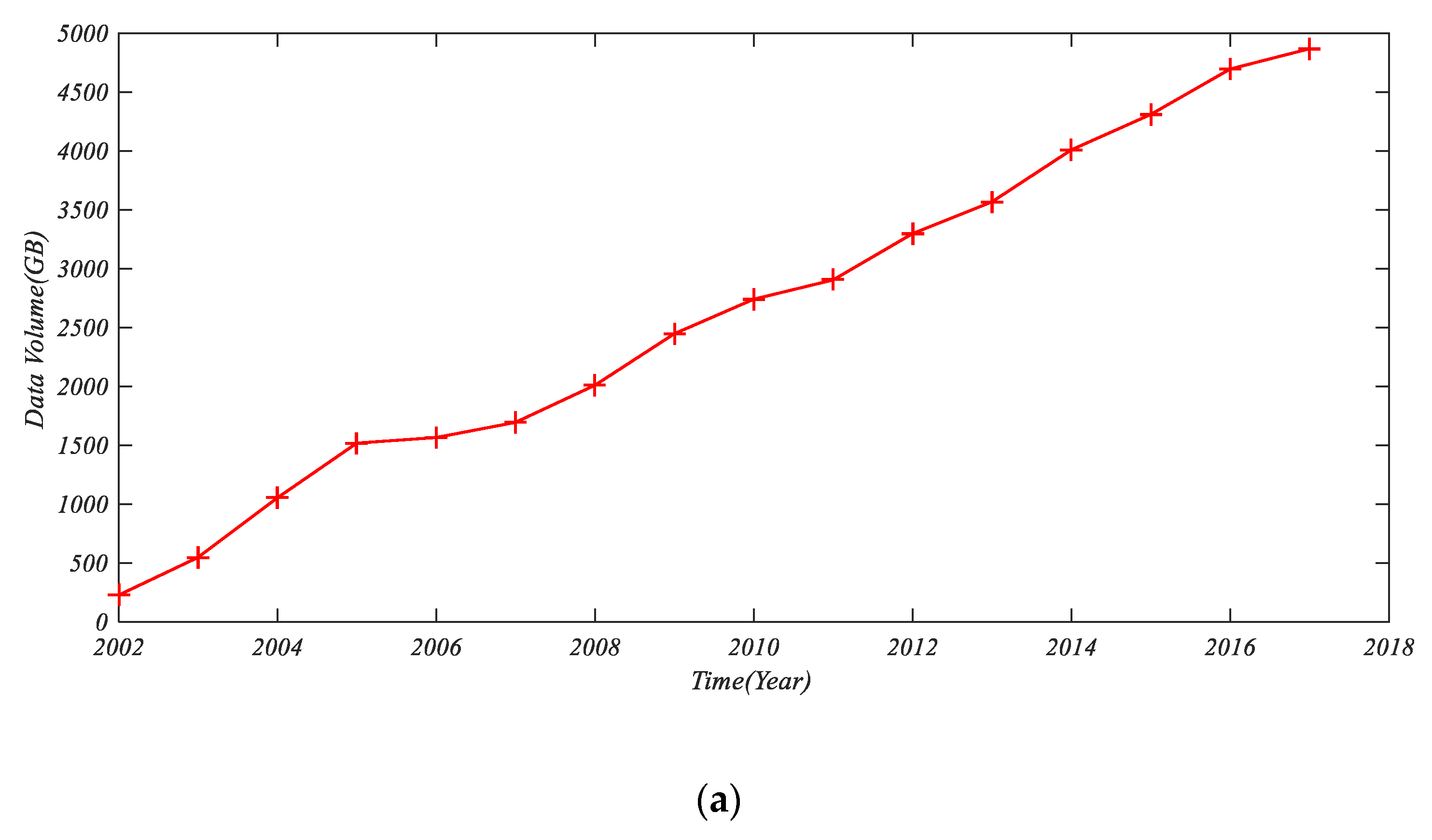
2.1. Current Situation

Since the establishment of Iran’s electricity market (IEM) in Iran (2002), databases of the electricity market have been storing data at the same time as when electricity is bought and sold. Such data are based on the activities of sellers and buyers in a certain field. The electricity market manager acts as an interface to receive data from buyers and sellers with the purpose of predicting and approving the fair price of electricity for the following day after electric load supply and demand forecasting. By 2017, There were over 25 parameters stored in databases of the electricity market for electricity price forecasting. The stored data indicate the actions of buyers and sellers, summarized in

Table 1. Stored parameters of IEM databases.

Parameter	Description	Comments	Data Storage Intervals	Domain (D)	Size of Stored Data for Total GB Calculation
P1	Average electricity consumption at the peak hour	This index was calculated for 39 power distribution companies separately. This parameter shows the mean.	Every Minute	[25,000, 40,000]	63.67
P2	Average electricity consumption at the peak hour last year	This index was calculated for 39 power distribution companies separately. This parameter shows the mean.	Every Minute	[25,000, 40,000]	64.43
P3	Total power exports	This index was stored for 201 power plants separately. This parameter indicates the mean.	Every Minute	[100, 2000]	378.87
P4	Total power imports	This index was stored for 201 power plants separately. This parameter shows the mean.	Every Minute	[10, 1000]	345.66
P5	Total power exchange	This index was stored for 201 power plants separately. This parameter shows the mean.	Every Minute	[100, 3000]	378.9
P6	Air temperature	-	Every Minute	[−15, 42]	12.45
P7	Cost of using network equipment	This index was calculated for 39 power distribution and 16 power transfer companies separately. This parameter shows the mean.	Every Minute	[2500, 4500]	87.78
P8	Cost of energy consumed by the network	This index was calculated for 39 power distribution and 16 power transfer companies separately. This parameter indicates the mean.	Every Minute	[2500, 5600]	74.43
P9	Cost of overseas exchange	This index was stored for 201 power plants separately. This parameter shows the mean.	Every Minute	[3000, 4000]	346.88
P10	Cost of energy provided for buyers in the market	This index was calculated for 39 power distribution companies separately. This parameter indicates the mean.	Every Minute	[150,000, 200,000]	56.67
P11	Buyers’ share in the use of services (Rial)	This index was calculated for 39 power distribution and 16 power transfer companies separately. This parameter shows the mean.	Every Minute	[20,000, 40,000]	78.67
P12	Cost of buying the active power consumption (Rial)	This index was calculated for 39 power distribution companies separately. This parameter shows the mean.	Every Minute	[1500, 4000]	57.76
P13	Buyers’ share in the cost of transfer services (Rial)	This index was calculated for 39 power distribution companies separately. This parameter indicates the mean.	Every Minute	[20,000, 40,000]	62.32
P15	Share of readiness	This index was stored for 201 power plants separately. This parameter indicates the mean.	Every Minute	[100, 150]	344.43
P16	Delayed sums of power plants	This index was stored for 201 power plants separately. This parameter indicates the mean.	Every Minute	[1500, 2500]	340.43
P17	Productivity coefficient of the power plant	This index was stored for 201 power plants separately. This parameter shows the mean.	Every Minute	[0.3, 1]	360.8
P18	Rates of extra services	This index was calculated for 39 power plants and 16 power transfer companies separately. This parameter shows the mean.	Every Minute	[2000, 6000]	79.93
P19	Sales proposition steps	This index was stored for 201 power plants separately. This parameter shows the mean.	Every Minute	[7000, 22,000]	340.9
P20	Modified coefficients of consumers	This index was calculated for 39 power distribution companies separately. This parameter indicates the mean.	Every Minute	[0.3, 0.9]	67.77
P21	Productivity coefficients of power plants	This index was stored for 201 power plants separately. This parameter indicates the mean.	Every Minute	[0.3, 0.98]	305.63
P22	Average thermal value	This index was stored for 201 power plants separately. This parameter shows the mean.	Every Minute	[20,000, 40,000]	345.32
P23	Coefficient of readiness cost	This index was stored for 201 power plants separately. This parameter shows the mean.	Every Minute	[0.3, 1]	305.81
P24	Noncooperation fine	This index was calculated for 39 power distribution and 16 power transfer companies separately. This parameter indicates the mean.	Every Minute	[100, 500]	51.61
P25	Sums of noncooperation	This index was calculated for 39 power distribution and 16 power transfer companies separately. This parameter shows the mean.	Every Minute	[2000, 4500]	50.77

.

The total size of generated data has been 10,158 GB since the establishment of the electricity market (up to 2017). It is predicted that 21,116 GB of data will be generated until 2022 (without considering the implementation of the smart grid). Moreover, the data generation rate of Iran’s electricity market is so high that the data of every parameter are stored in every minute. Regarding Big Data, validity and variety are important in addition to the size and rate of data generation. According to the data verification at different levels of power supply chain compared with previously real and estimated data on average, the generated data indicated uncertainty. Data uncertainty is a feature of Big Data [51]. In the next step, the data of electricity market and varied data are searched. Such a variety includes nominal, ordinal, and numeral data in addition to dates and time. Figure 2 indicates the four features.

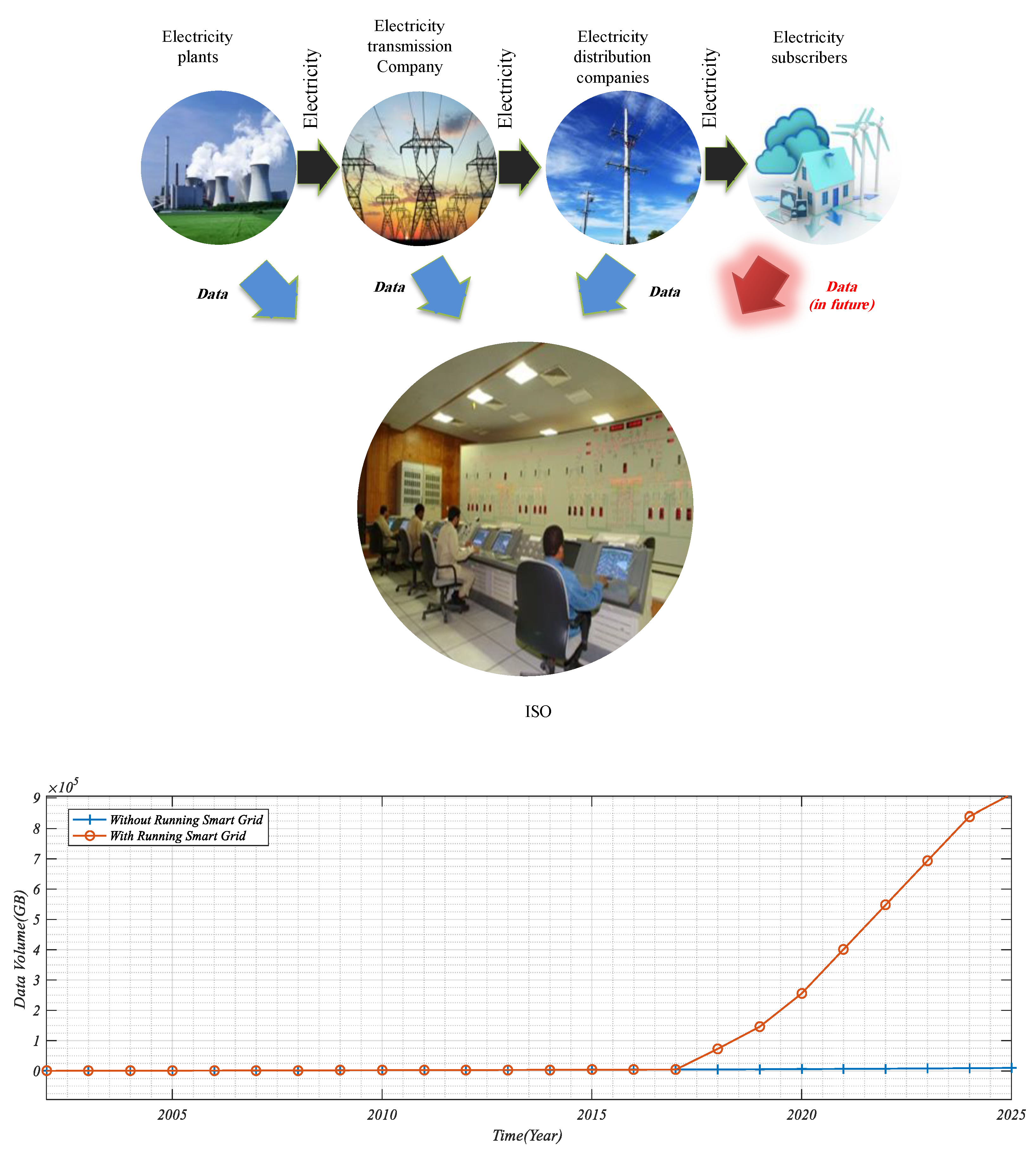
2.2. State of the Future

Given the changes in the electricity market to create smart grids and welcome retail buyers and retailers in the market, data generation rate has greatly increased so much that data will be recorded instantly [14]. Therefore, if the smart grid is implemented thoroughly across Iran (from 2018 to 2025) to gradually cover over 33,689,000 home and industrial electricity subscribers, it is predicted that 2.5 terabytes of data will be generated daily. As a result, there will be unbelievably numerous sources of data generation. In fact, every home or building will turn into a data generation source in the market (Figure 3) [52]. Therefore, Iran’s electricity market will include a very great amount of data, and the daily-generated data of the smart grid may amount to the monthly-generated data of the ordinary market. Thus, the structures of data storage and analysis should be prepared for great developments of data generation in the foreseeable future. Certain methods should also be proposed to exploit the potential of previous Big Data, indicating the performance of relevant actors and different states of the market with the purpose of predicting the important variables more accurately.

3. Components of the Algorithm

3.1. Wavelet

A wavelet is a series of mathematical functions used to decompose a continuous signal into frequency components. The resolution of each component is equal to its scale. The decomposition wavelet transform is a function based on wavelet functions. Wavelets (also known as daughter wavelets) are the samples transferred and scaled from a function (a mother wavelet) [24]. They are characterized by finite lengths and highly mortal oscillations. The following figure shows a few mother wavelets. The continuous wavelet transform converts a continuous function of time into the time-frequency space. The bases of the new space are wavelet functions. In mathematics, a continuous wavelet transform is defined as a continuous function like x(t), the squared version of which is integrable (a > 0, $R ϵ b$). Equation (1) shows such a wavelet:

$$CW{T}_x \left(a.b\right)= \frac{1}{\sqrt{\left|a\right|}} \underset{-\infty }{\overset{\infty }{{\displaystyle \int }}}x\left(t\right) {\Psi }^{*}\left(t\right) x\left(t\right)dt$$

(1)

In this equation, $\Psi$ is a continuous function in time and frequency, t shows the signal length of x(t). The transfer and scale parameters include the continuous values of m and n, for which a = 2^m and a = 2ⁿ. It is known as the mother wavelet, defined as Equation (2):

$${\Psi }_{a.b}\left(t\right)=\frac{1}{\sqrt{a}} \left(\frac{t-b}{a} \right)$$

(2)

In a discrete wavelet transform, a signal is passed through a series of overpass filters for high-frequency analysis and a series of underpass filters for low-frequency analysis. A signal is divided into two parts, one of which results from the passage of signal through the overpass filter including high-frequency information (such as noise). It is called the details. The other part results from the passage of signal through an underpass filter including low-frequency information and the identity properties of the signal. The second part is called generalities and shown as Equation (3):

$$DW{T}_x \left(m.n\right)= 2^{-\left(\frac{m}{2}\right)} {\displaystyle \sum }_{t=0}^{T-1}\underset{-\infty }{\overset{\infty }{{\displaystyle \int }}}x\left(t\right) \Psi \left( \frac{t-n{2}^m}{2^m}\right) dt$$

(3)

The Haar wavelet is a specific series of functions known as the first wavelet. There are several methods of wavelet transforms, the simplest of which is the Haar wavelet. In this paper, it was used in three steps. There are also other methods such as db2 and db4, used in other papers. The Haar mother wavelet is defined as Equation (4):

$$\Psi \left(t\right)=\{\begin{array}{c}1 0\le t<\frac{1}{2} \\ 0 otherwise \\ -1 \frac{1}{2} \le t <1\end{array}$$

(4)

The comparing function is shown by Equation (5):

$$\Psi \left(t\right)= \{\begin{array}{c}1 0\le t <1\\ 0 otherwise \end{array}$$

(5)

The decomposition steps are shown in Figure 4. Equation (6) indicates the stepwise decomposition equations.

D = A₁ + D₁
= D₁ + D₂ + A₂
= D₁ + D₂ + D₃ + A₃

(6)

After applying the neural network to the set of problem inputs, As and Ds were combined with each other to calculate and predict supply (S) and demand (D). Figure 5 shows the combination these components. In other words, they result from the inversed version of Equation (6).

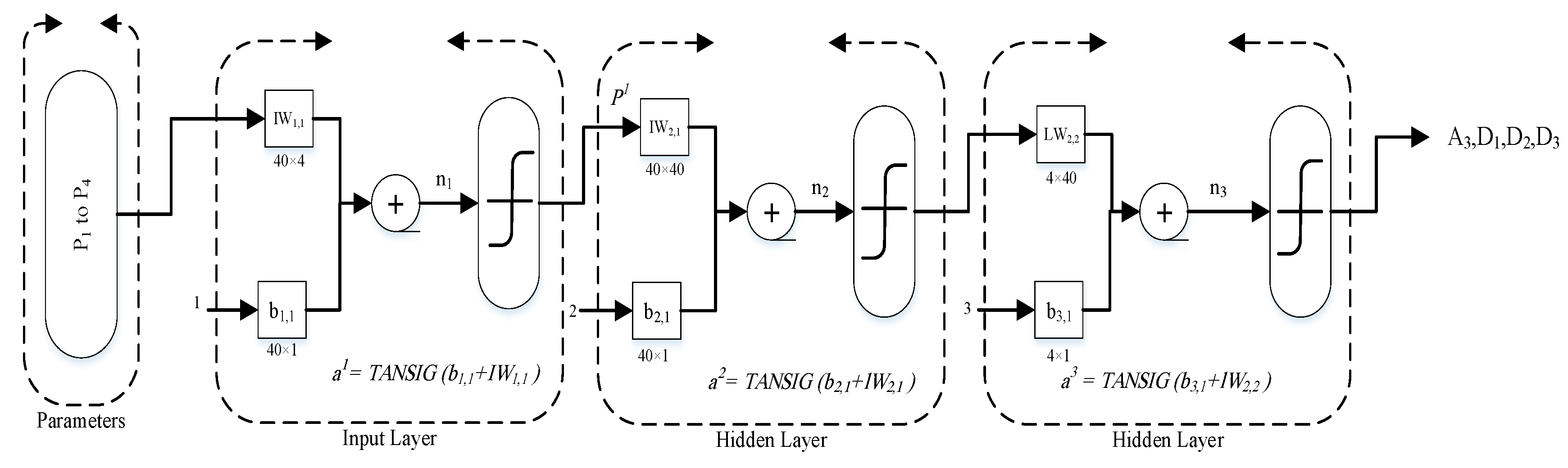
3.2. Neural Network Particle Swarm Optimization (NNPSO)

The Back-propagation neural network (BPNN) is a kind of multilayer neural network with a nonlinear transfer function and Widrow-Hoff learning rules. The input and target vectors are used to train this type of the network for estimating a function, finding a relationship between inputs and outputs, and classifying inputs. A BP network has a bias to estimate every function with the limited number of discontinuities. BP is a standard algorithm characterized by reduced gradient. In BP, network weights move in the opposite direction of the efficiency function gradient. The term back-propagation refers to the behavior of a BP network in gradient calculation for multilayer nonlinear networks. There are different algorithms operating based on the standard BP algorithm such as the conjugate gradient algorithm and Newton’s method. The most common BP network architecture is the feed forward network [23]. Figure 6 shows a simple neuron with R inputs:

The tansig function can be used to generate inputs ranging between −1 and 1. If the last layer of a multilayer network has sigmoid neurons, the output is limited to a shorter range. However, if linear neurons are used, the output can have any value.

The feed forward networks often have one or several hidden layers of sigmoid neurons by using a linear terminal layer. The presence of several layers of neurons and a nonlinear tansig function enables the network to learn about linear and nonlinear relationships between inputs and outputs. The linear output layer enables the network to have inputs outside the expected range. However, if the output exists in the expected range, the logsig function is used in the linear layer. In the example of this article, Figure 7 indicates the structure of a feed forward network with tansig functions and two layers of 40 neurons.

Table 2. BPNN parameters.

Parameter	Value
Number of neurons in hidden layer	40
Learning coefficient	0.9
Momentum	0.2
Activation functions in hidden layer	TANSIG
Activation functions in output layer	TANSIG
Length of training data	180, 360, 720, 1440
Training function	TRAINLM
Number of epochs	1000

indicates the implementation parameters of the neural network.

In this technique, PSO is used to train the neural network. The PSO is a global minimization method which can be employed to deal with certain problems, to which solutions include a point or surface of the n-dimensional space. In such a space, there are certain assumptions with an initially-allocated speed [26]. There are also communication channels between particles. Then the particles flow across the solution space, and results are calculated on the basis of a qualification criterion in every interval. With the passage of time, particles move towards the other particles with higher qualification criteria in the same communication group (Figure 8).

The position and initial velocity of particles can be calculated through Equations (7) and (8), respectively. The velocity, weight (w), and position of particles can be obtained from Equations (9), (10), and (11) in every iteration.

Table 3. PSO parameters.

Parameter	Value
Swarm size	60
Initial weight w1	0.9
Final weight w2	0.4
ϕ1, ϕ2	2, 2
Max. number of iterations	1000

indicates the input parameters required to implement the PSO algorithm in neural network training.

$$x_0^i=x_{min}+rand \left( x_{max}- x_{min}\right)$$

(7)

$$v_0^i=\frac{x_{min}+rand \left(x_{max}- x_{min}\right)}{\Delta t}$$

(8)

$$v_{t+1}^i=w v_t^i+{\mathsf{\varphi }}_{1}ran{d}_1 \left( \raisebox{1ex}{$p_t{}^i-x_t^i$}\!\left/ \!\raisebox{-1ex}{$\Delta t$}\right.\right)+ {\mathsf{\varphi }}_{2}ran{d}_2 \left( \raisebox{1ex}{$p_t^g-x_t^i$}\!\left/ \!\raisebox{-1ex}{$\Delta t$}\right.\right)$$

(9)

$$w=\left( w_1-w_2 \right)\frac{ite{r}_{max}-iter}{ite{r}_{max}}+w_2$$

(10)

$$x_{t+1}^i= x_t^i+v_{t+1}^i \Delta t$$

(11)

where $x_0^i$ is the current position of the particle, x_min and x_max are, respectively, the minimum and maximum coordinates of the particle i, $v_0^i$ is the initial velocity of particle i, $v_{t+1}^i$ is the velocity of particle i at t + 1, ϕ₁ and ϕ₂ are the coefficients of motion tendency adjustment towards global optimal or best solution obtained by particle i, $p^i$ is the best position experienced by particle i, $p_t^g$ is the best position experienced by all particles until t; and $x_t^i$ is the position of particle i at t.

3.3. Simulation-Optimization

3.3.1. Monte Carlo Simulation

The Monte Carlo method is a computational algorithm using the random sampling to obtain results. The Monte Carlo methods are usually employed to simulate physical, mathematical, and economic systems. Such methods are often used when a mathematical or physical system is being simulated. Since they rely on iterative computations and random or false-random numbers, the Monte Carlo methods are often adjusted in a way that they can be executed by computers. In this study, the Monte Carlo simulation was used to select previous Big Data at random and compute the objective function and values of supply and demand generated in every step of the PSO algorithm.

Table 4. Monte Carlo simulation parameters.

Parameter	Description	Value
n	Number of simulations	1000
l	The size of each simulation	100
DP1	Average electricity consumption at the peak hour Domain	[25,000, 40,000]
DP2	Average electricity consumption at the peak hour last year Domain	[10, 1000]
DP3	Total power imports Domain	[25,000, 40,000]
DP4	Total power exchange Domain	[100, 2000]

shows the simulation parameters of this method.

3.3.2. PSO

The PSO was introduced in Section 3.2. This algorithm will also be used in the simulation-optimization conducted on previous Big Data.

Table 5. Execution parameters of PSO.

Parameter	Value
Swarm size	100
Initial weight w1	0.9
Final weight w2	0.4
ϕ1, ϕ2	2, 2
Max. number of iterations	1000
$\alpha ,\beta$	0.6, 0.4

indicates the input parameters of PSO used for preprocessing data.

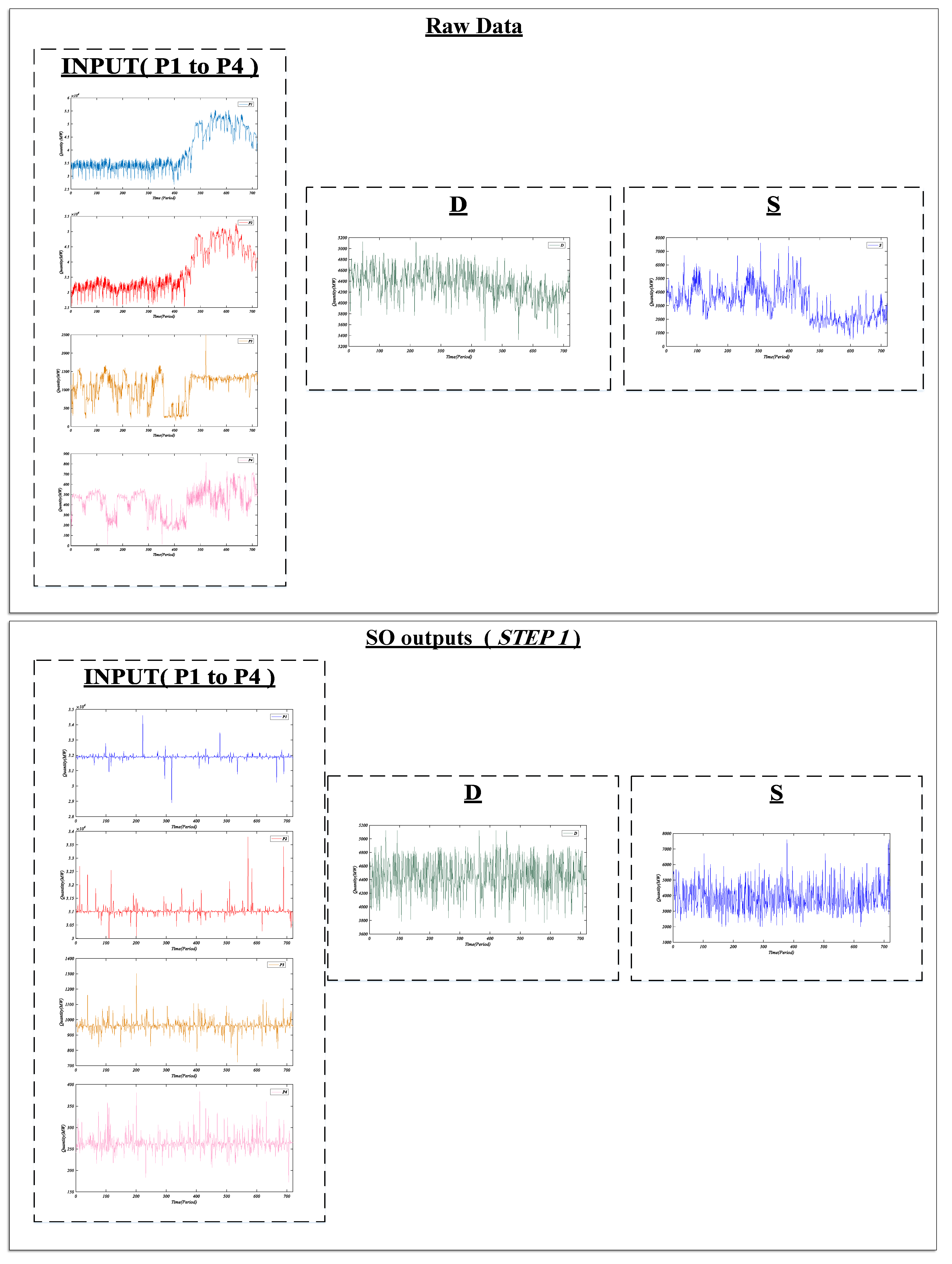
3.3.3. Simulation-Optimization (SO) Algorithm

First, it is necessary to point out that the problem of generating solutions close to the current solution is classified as the knapsack or rucksack problem. Such problems are solved by using metaheuristic algorithms because they are considered hard problems [53]. Now the knapsack problem is described briefly.

Known as the knapsack or rucksack problem, it is combinatorial optimization problem. Assume that a group of objects is available with specific versions or values. Every object is allocated a certain number so that the weights of selected objects are smaller or equal to a predetermined limit; however, values are maximized.

Assume that there are n objects, numbered from 1 to n. The value of ith object is v_i, and its weight is w_i. It is usually assumed that weights and values are nonnegative. For a simpler presentation, it can be assumed that objects are sorted in an ascending order of weights without damaging the problem generality. The maximum weight that can be carried in a knapsack is W.

The most famous type of such a problem is the 0 and 1 knapsack problem. In other words, there is zero of every object (not selected) or one of every object (selected). The 0 and 1 knapsack problem can be stated mathematically:

$$\mathrm{Maximize}\mathrm{the}\mathrm{value}\mathrm{of}{\sum }_{i=1}^n{v}_i{x}_i\mathrm{in}\mathrm{a}\mathrm{way}\mathrm{that}{\sum }_{i=1}^n{w}_i{x}_i\le W,x_i\in \left\{0,1\right\}.$$

The bounded knapsack problem is another version in which the number of objects is a real and nonnegative value. It is equal to c_i at the most. In mathematical terms, ${\sum }_{i=1}^n{v}_i x_i$ should be maximized in a way that ${\sum }_{i=1}^n{w}_i x_i \le W , x_i \in \left[0,c_i\right]$. In this study, the values of input parameters were selected with the assumption that their values and weights were equal. The values were selected in the minimum-to-maximum range of every parameter. However, a variance y_i was used in the objective function to prevent the convergence of all solutions to a specific group of values:

$$v_{i }=1 , w_i=1 , Min\left(P_i\right)\le x_i \le Max\left(P_i\right) \forall i$$

The goal of executing simulation-optimization on the big data of the electricity market was to find the initial solutions with the least variation from the current parameters ($z_{current}=(z_1.\cdots .z_m$)). Given the fact that it is not possible to form a specific model between the time and values of input parameters, simulation was used to calculate the values of the objective function and predict supply and demand based on random points selected for the new points generated by the PSO. The hybrid of simulation and optimization can analyze Big Data of the electricity market at a high speed. Therefore, the sets of initial solutions can be added into the wavelet-PSO-NNs model (Figure 9).

In this algorithm, the initial population is generated first by the PSO. New populations are generated in accordance with the steps described in Section 3.3.2. The Monte Carlo simulation method was used to calculate the value of the fitness function. According to Section 3.3.1, a set of random populations is generated first based on time. Then the values of objective function, supply, and demand are calculated by considering the difference between the current solution ($z_{current}=\left(z_1.\cdots .z_m\right)$) and random solutions selected in the P step of PSO (y_p = (y₁, y₂, ..., y_m)). Figure 10 shows the necessary equations. Then the value of fitness function and predicted values of supply and demand were given back to the PSO to resume simulation. The algorithm would be terminated, if the maximum number of iterations were achieved (Table 5). The steps are taken separately for supply and demand values.

4. The Wavelet-NNPSO Algorithm

The goal of this model is to combine the SO method with the Wavelet-NNPSO (WT-NNPSO) algorithm to search in the previous Big Data and to select the best initial solutions used as the inputs of the WT-NNPSO for more accurate forecasting of supply and demand variables. Figure 11 shows the steps in the implementation of this algorithm

Step 1. The data are analyzed by the SO algorithm (Section 3.3). The best selected solutions are in the closest status to current parameters. This algorithm is able to search in the previous Big Data of the electricity market. Such an extensive search is conducted in a limited interval because it is smart. This algorithm is run until the termination condition is met. After that, the predicted values of S and D are entered into Step 2.

Step 2. In this step, the time series of the previous step are decomposed by the Haar wavelet transform. The decomposition is done through equations introduced in Section 3.1.

Step 3. Based on the data analyzed in Step 2, certain weights are determined for parameters through neural networks and PSO. This step is kept on until the number of algorithm execution reaches 1000 (the number of epochs). Then the algorithm is terminated.

Step 4. In this step, the wavelet is combined so that the values of supply and demand can be predicted. The output values are the best values predicted for supply and demand ($S_t{}^{Forcast}$ and $D_t{}^{Forcast}$).

5. Numerical Results and Discussion

5.1. An Instance of the New Technique

The results of predicting supply and demand were obtained from coding and implementing the algorithm in Matlab R16a^® (USA, California)(‘nftool’, ‘wavemenue’). Figure 12 shows the inputs and components decomposed in the Haar wavelet for the first future interval and LOTD = 720.

5.2. Analyzing the Accuracy and Speed of the New Technique

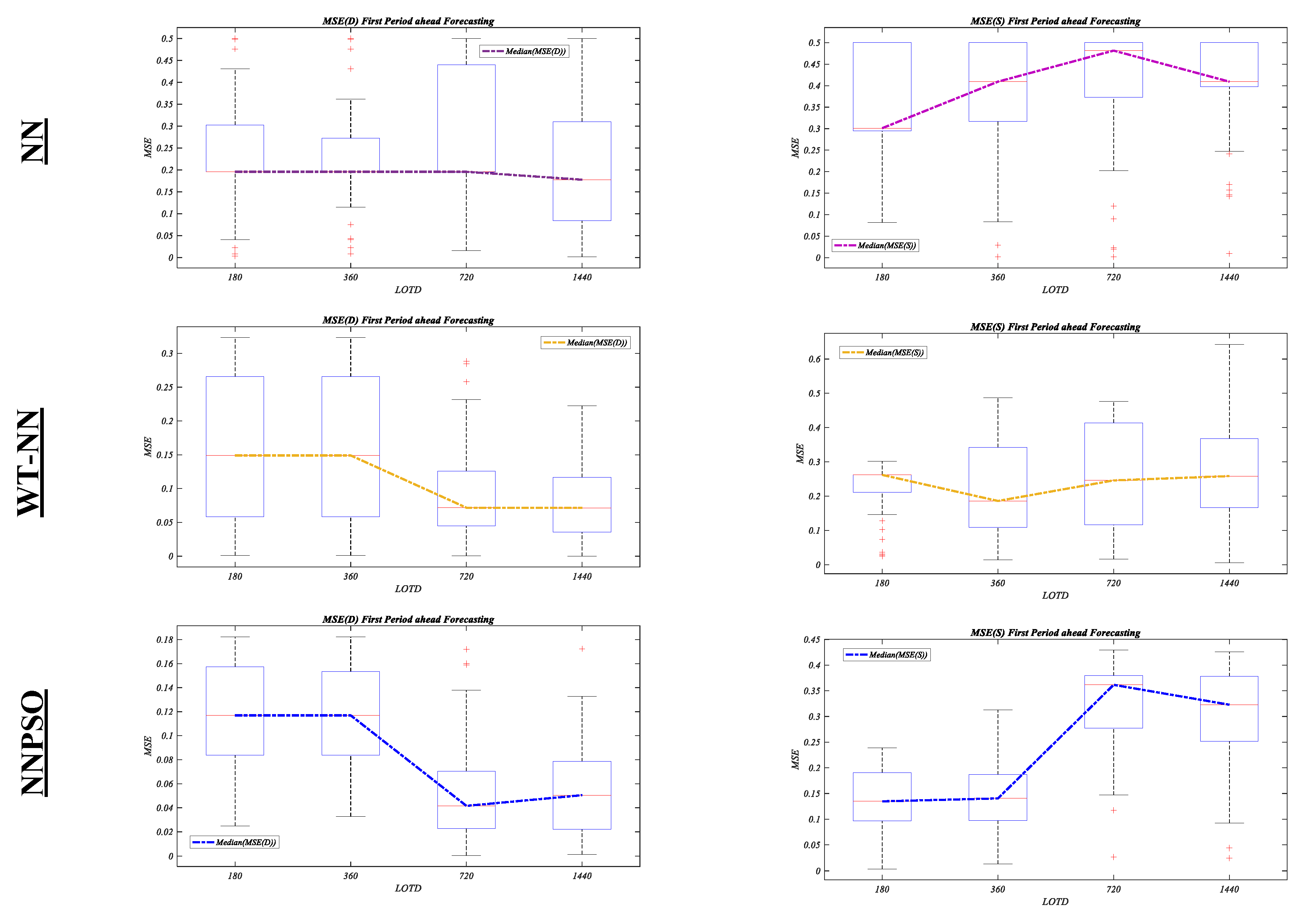
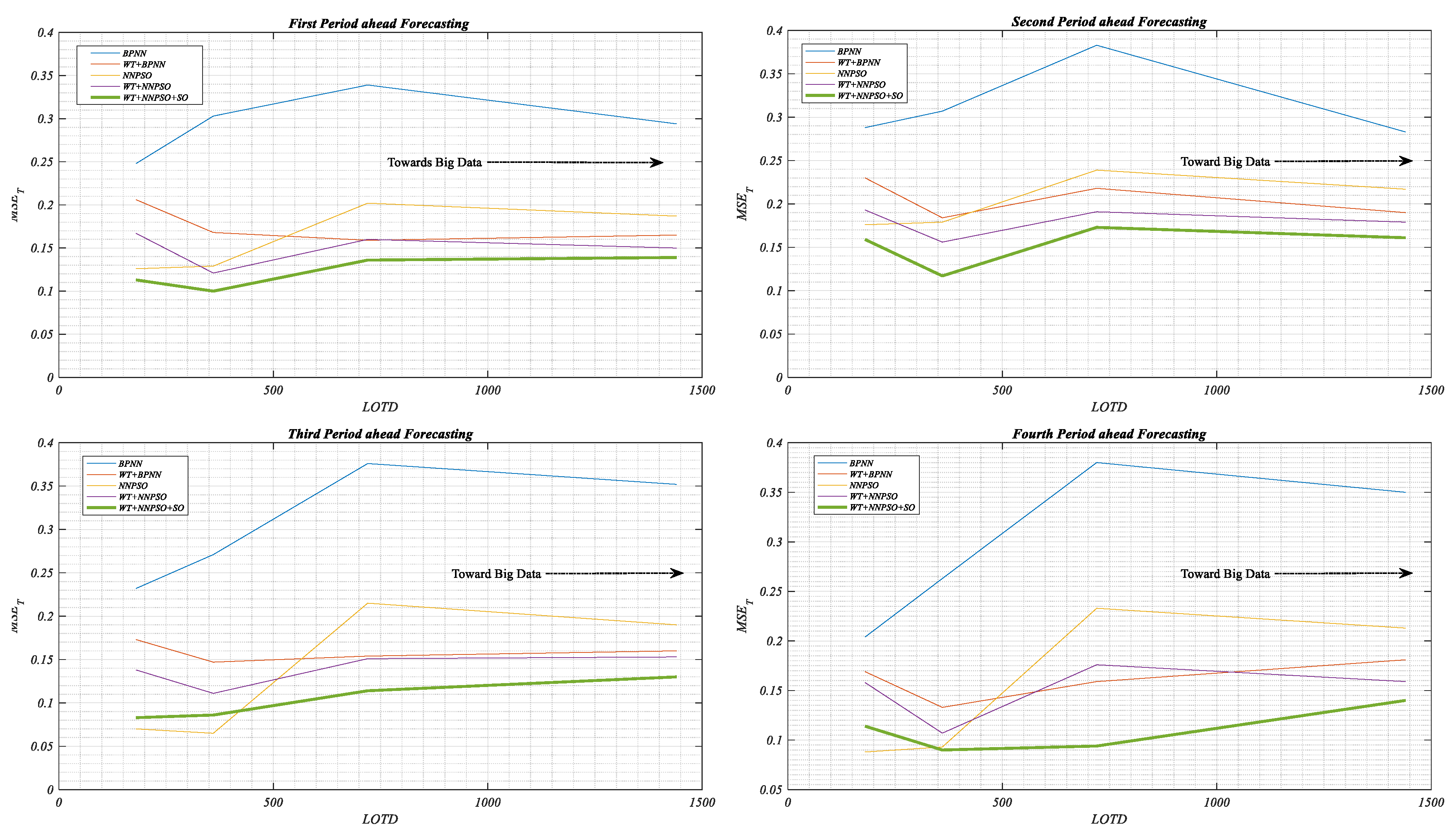
5.2.1. The Implementation Accuracy

In this paper, the mean squared error (MSE) was used to compute and compare errors. RMSE is calculated to predict supply, demand, and the average summation of supply and demand. Equations (12)–(14) show how RMSE is calculated:

$$MS{E}_S=\frac{1}{N}\sqrt{{\displaystyle \sum }_{t=1}^T{\left(\frac{S_t{}^{Actual}-S_t{}^{Forcast} }{S_t{}^{Actual}}\right)}^2}$$

(12)

$$MS{E}_D=\frac{1}{N}\sqrt{{\displaystyle \sum }_{t=1}^T{\left(\frac{D_t{}^{Actual}-D_t{}^{Forcast} }{D_t{}^{Actual}}\right)}^2 }$$

(13)

$$MS{E}_T=\left(MS{E}_S+ MS{E}_D\right)/2$$

(14)

Here $S_t{}^{Actual}$ and $D_t{}^{Actual}$ show the actual values of supply and demand at t, respectively. Such data were obtained through coding new techniques in Matlab R16a^® (Natick, MA, USA). The forecasting errors of the new technique were compared with those of the older ones, in which wavelet transforms or metaheuristic algorithms were not used. The new and old techniques were different in LOTD.

Table 6. Error comparison for different models in the first future interval (LOTD = 180, 360, 720, 1440).

LOTD	Error	Model
		BPNN	WT+BPNN	NNPSO	WT+NNPSO	WT-NNPSO+SO
180	$MS{E}_D$	0.196	0.149	0.117	0.089	0.084
	$MS{E}_S$	0.302	0.262	0.135	0.244	0.141
	$MS{E}_T$	0.248	0.206	0.126	0.167	0.113
360	$MS{E}_D$	0.196	0.149	0.117	0.089	0.089
	$MS{E}_S$	0.409	0.186	0.141	0.153	0.111
	$MS{E}_T$	0.303	0.168	0.129	0.121	0.1
720	$MS{E}_D$	0.196	0.072	0.042	0.064	0.089
	$MS{E}_S$	0.482	0.246	0.362	0.255	0.182
	$MS{E}_T$	0.339	0.159	0.202	0.16	0.136
1440	$MS{E}_D$	0.178	0.071	0.05	0.074	0.101
	$MS{E}_S$	0.409	0.259	0.323	0.226	0.176
	$MS{E}_T$	0.294	0.165	0.187	0.15	0.139

,

Table 7. Error comparison for different models in the second future interval (LOTD = 180, 360, 720, 1440).

LOTD	Error	Model
		BPNN	WT-BPNN	NNPSO	WT-NNPSO	WT-NNPSO-SO
180	$MS{E}_D$	0.281	0.228	0.193	0.159	0.15
	$MS{E}_S$	0.294	0.232	0.159	0.227	0.168
	$MS{E}_T$	0.288	0.23	0.176	0.193	0.159
360	$MS{E}_D$	0.282	0.188	0.186	0.174	0.144
	$MS{E}_S$	0.331	0.18	0.172	0.137	0.119
	$MS{E}_T$	0.307	0.184	0.179	0.156	0.117
720	$MS{E}_D$	0.282	0.17	0.105	0.12	0.143
	$MS{E}_S$	0.483	0.265	0.374	0.261	0.203
	$MS{E}_T$	0.383	0.218	0.239	0.191	0.173
1440	$MS{E}_D$	0.18	0.137	0.097	0.116	0.167
	$MS{E}_S$	0.385	0.243	0.337	0.242	0.155
	$MS{E}_T$	0.283	0.19	0.217	0.179	0.161

,

Table 8. Error comparison for different models in the third future interval (LOTD = 180, 360, 720, 1440).

LOTD	Error	Model
		BPNN	WT+BPNN	NNPSO	WT+NNPSO	WT+NNPSO+SO
180	$MS{E}_D$	0.047	0.117	0.026	0.053	0.035
	$MS{E}_S$	0.416	0.228	0.113	0.222	0.13
	$MS{E}_T$	0.232	0.173	0.07	0.138	0.083
360	$MS{E}_D$	0.041	0.044	0.026	0.041	0.035
	$MS{E}_S$	0.5	0.249	0.104	0.181	0.137
	$MS{E}_T$	0.271	0.147	0.065	0.111	0.086
720	$MS{E}_D$	0.251	0.051	0.088	0.073	0.032
	$MS{E}_S$	0.5	0.256	0.342	0.228	0.195
	$MS{E}_T$	0.376	0.154	0.215	0.151	0.114
1440	$MS{E}_D$	0.204	0.061	0.082	0.079	0.042
	$MS{E}_S$	0.5	0.259	0.298	0.226	0.218
	$MS{E}_T$	0.352	0.16	0.19	0.153	0.13

and

Table 9. Error comparison for different models in the fourth future interval (LOTD = 180, 360, 720, 1440).

LOTD	Error	Model
		BPNN	WT+BPNN	NNPSO	WT+NNPSO	WT+NNPSO+SO
180	$MS{E}_D$	0.053	0.091	0.06	0.081	0.065
	$MS{E}_S$	0.354	0.246	0.115	0.234	0.163
	$MS{E}_T$	0.204	0.169	0.088	0.158	0.114
360	$MS{E}_D$	0.056	0.06	0.062	0.069	0.061
	$MS{E}_S$	0.469	0.206	0.124	0.145	0.119
	$MS{E}_T$	0.263	0.133	0.093	0.107	0.09
720	$MS{E}_D$	0.28	0.072	0.113	0.107	0.032
	$MS{E}_S$	0.48	0.246	0.353	0.244	0.156
	$MS{E}_T$	0.38	0.159	0.233	0.176	0.094
1440	$MS{E}_D$	0.23	0.093	0.114	0.115	0.05
	$MS{E}_S$	0.47	0.268	0.311	0.203	0.23
	$MS{E}_T$	0.35	0.181	0.213	0.159	0.14

show the root median squared error obtained from 100 executions of the new technique. The results include forecasting for one to four future intervals.

Figure 13 indicates the boxplot of the forecasting in the first future interval for different LOTDs and other methods.

Figure 14 shows the MSE_T in the first to fourth future intervals.

According to Figure 14, the new technique resulted in the best predicted values for the first to fourth future intervals. On average, the values were 0.028, 0.045, 0.035, and 0.040, respectively, for different LOTDs. Such a comparison can be drawn in more LOTDs or parameters. According to the results, it is predicted that the new technique will maintain performance in higher LOTDs.

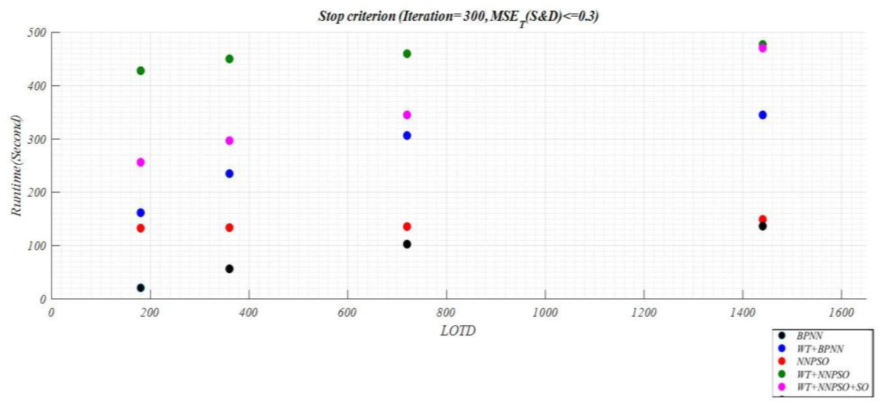
5.2.2. The Speed of the New Technique

The implementation speed will become more important when the smart grid is thoroughly established in the electricity market. In addition to increasing the accuracy, the newly proposed method will take less time to find a solution, something which really matters to the electricity market manager due to the increase speed of electricity price forecasting. Figure 15 shows the implementation speed of the new technique and other methods in constant termination conditions (0.3 ≤ MSE and max. iteration = 300) for supply and demand on average. Accordingly, the new technique improved the implementation time in comparison with WT+NNPSO. In other words, the forecasting time reduced by 90.66 s for different LOTDs on average. Such a reduction was observed at the same time as an increase in accuracy, discussed in Section 5.2.1.

Figure 16 also shows by increasing the data under investigation, improved speed, and accuracy of the algorithm are preserved. The diameter of the circle represents MSE_T.

5.2.3. Summary of Results

Comparing the speed and accuracy of the new algorithm and available algorithms shows that by increasing the amount of data under investigation, the accuracy of the new algorithm is maintained while simultaneously the slope of the execution time of the new algorithm is lower than the existing algorithms. These results show that the big data analysis of the electricity market has good results with the new algorithm in future. With the introduction of a global network of smart grids, the electricity market manager needs to use pre-processing algorithms more than ever before.

6. Conclusions and Suggestions

According to the results of a case study conducted on the database of Iran’s electricity market, there have been great sizes of Big Data stored since 2002. The future changes of Iran’s electricity structure indicate that there will be very much greater data in the market than ever before after establishing smart grids thoroughly across Iran in the presence of retail buyers and retailers. In this problem, it was assumed that the use of previous big stored data would be effective in the better forecasting of important variables, i.e., supply and demand. Therefore, neural network techniques were developed along with one of the simulation-optimization algorithms (PSO-Monte Carlo) to improve the ability of current techniques to predict big variables of the electricity market and reduce the implementation time in the presence of such variables. According to the results, there is appropriate information in the big sizes of data stored in the electricity market. The forecasting of important variables can be improved by conducting appropriate search in data. However, it is necessary to employ metaheuristic algorithms due to the big sizes of data. Given the lack of a specific model for establishing relationships between current parameters and data storage time, simulations were conducted to obtain the objective function and predict the values of supply and demand. It is suggested that other Big Data analysis methods, one of which is machine learning, should be developed and used in short-term electrical load forecasting techniques. It is also suggested that the proposed technique be combined with the fuzzy logic. In general, due to the restructuring of the electricity market in the world, it is recommended to use methods that have high speed and precision in prediction. Furthermore, some suggestions are made for future studies:

• Using other intelligent meta-heuristic methods for selecting the input data of neural networks (making data selection more intelligent).
• Employing the fuzzy logic in the newly proposed model.

References

1. Debnath, K.B.; Mourshed, M. Forecasting methods in energy planning models. Renew. Sustain. Energy Rev. 2018, 88, 297–325. [Google Scholar] [CrossRef]
2. Barbieri, F.; Rajakaruna, S.; Ghosh, A. Very short-term photovoltaic power forecasting with cloud modeling: A review. Renew. Sustain. Energy Rev. 2017, 75, 242–263. [Google Scholar] [CrossRef]
3. Taylor, J.W. An evaluation of methods for very short-term load forecasting using minute-by-minute British data. Int. J. Forecast. 2008, 24, 645–658. [Google Scholar] [CrossRef] [Green Version]
4. Panapakidis, I.P. Clustering based day-ahead and hour-ahead bus load forecasting models. Int. J. Electr. Power Energy Syst. 2016, 80, 171–178. [Google Scholar] [CrossRef]
5. Yang, H.Y.; Ye, H.; Wang, G.; Khan, J.; Hu, T. Fuzzy neural very-short-term load forecasting based on chaotic dynamics reconstruction. Chaos Solitons Fractals 2006, 29, 462–469. [Google Scholar] [CrossRef]
6. Ahmad, T.; Chen, H. Short and medium-term forecasting of cooling and heating load demand in building environment with data-mining based approaches. Energy Build. 2018, 166, 460–476. [Google Scholar] [CrossRef]
7. Shikhah, N.A.; Elkarmi, F. Medium-term electric load forecasting using singular value decomposition. Energy 2011, 36, 4259–4271. [Google Scholar] [CrossRef] [Green Version]
8. Bello, A.; Reneses, J.; Muñoz, A.; Delgadillo, A. Probabilistic forecasting of hourly electricity prices in the medium-term using spatial interpolation techniques. Int. J. Forecast. 2016, 32, 966–980. [Google Scholar] [CrossRef]
9. Yalcinoz, T.; Eminoglu, U. Short term and medium term power distribution load forecasting by neural networks. Energy Convers. Manag. 2005, 46, 1393–1405. [Google Scholar] [CrossRef]
10. De Felice, M.; Alessandri, A.; Catalano, F. Seasonal climate forecasts for medium-term electricity demand forecasting. Appl. Energy 2015, 137, 435–444. [Google Scholar] [CrossRef]
11. Carcedo, J.M.; García, J.P. Integrating long-term economic scenarios into peak load forecasting: An application to Spain. Energy 2017, 140, 682–695. [Google Scholar] [CrossRef]
12. Ali, D.; Yohanna, M.; Puwu, M.I.; Garkida, B.M. Long-term load forecast modelling using a fuzzy logic approach. Pac. Sci. Rev. Nat. Scie Eng. 2016, 18, 123–127. [Google Scholar] [CrossRef]
13. Ali, D.; Yohanna, M.; Ijasini, P.M.; Garkida, M.B. Application of fuzzy—Neuro to model weather parameter variability impacts on electrical load based on long-term forecasting. Alexan Eng. J. 2018, 57, 223–233. [Google Scholar] [CrossRef]
14. Chen, T.; Wang, Y.C. Long-term load forecasting by a collaborative fuzzy-neural approach. Int. J. Electr. Pow. Energy Syst. 2012, 43, 454–464. [Google Scholar] [CrossRef]
15. Chen, T. A collaborative fuzzy-neural approach for long-term load forecasting in Taiwan. Comput. Ind. Eng. 2012, 63, 663–670. [Google Scholar] [CrossRef]
16. Kang, J.; Zhao, H. Application of Improved Grey Model in Long-term Load Forecasting of Power Engineering. Syst. Eng. Procedia 2012, 3, 85–91. [Google Scholar] [CrossRef]
17. Marín, F.J.; Sandoval, F. Short-term peak load forecasting: Statistical methods versus artificial neural networks. In From Neuroscience to Technology Biological and Artificial Computation; Mira, J., Moreno-Díaz, R., Cabestany, J., Eds.; Springer: Berlin/Heidelberg, Germany, 1997; pp. 1334–1343. [Google Scholar]
18. Amral, N.; Ozveren, C.S.; King, D. Short term load forecasting using multiple linear regression. In Proceedings of the 42nd International Universities power Engineering Conference, Brighton, UK, 4–6 September 2007; pp. 1192–1198. [Google Scholar]
19. Chen, J.-F.; Wang, W.-M.; Huang, C.-M. Analysis of an adaptive time-series autoregressive moving-average (ARMA) model for short-term load forecasting. Electr. Power Syst. Res. 1995, 34, 187–196. [Google Scholar] [CrossRef]
20. Christiaanse, W.R. Short-term load forecasting using general exponential smoothing. IEEE Trans. Power Appar. Syst. 1971, PAS-90, 900–911. [Google Scholar] [CrossRef]
21. Chakhchoukh, Y.; Panciatici, P.; Mili, L. Electric load forecasting based on statistical robust methods. IEEE Trans. Power Syst. 2011, 26, 982–991. [Google Scholar] [CrossRef]
22. Raza, M.Q.; Baharudin, Z.; Islam, B.U.; Zakariya, M.A.; Khir, M.H.M. Neural network based STLF model to study the seasonal impact of weather and exogenous variables. Res. J. Appl. Sci. Eng. Technol. 2013, 6, 3729–3735. [Google Scholar] [CrossRef]
23. Li, S.; Wunsch, D.; O’Hair, E.; Glesselmann, M. Using neural networks to estimate wind turbine power generation. IEEE Trans. Energy Convers. 2001, 16, 276–282. [Google Scholar]
24. Xia, C.; Zhang, M.; Cao, J. A hybrid application of soft computing methods with wavelet SVM and neural network to electric power load forecasting. J. Electr. Syst. Inf. Technol. 2017. [Google Scholar] [CrossRef]
25. Irani, R.; Nasimi, R. Evolving neural network using real coded genetic algorithm for permeability estimation of the reservoir. Expert Syst. Appl. 2011, 38, 9862–9866. [Google Scholar] [CrossRef]
26. Zhaoyu, P.; Shengzhu, L.; Hong, Z.; Nan, Z. The Application of the Pso Based BP Network in Short-Term Load Forecasting. Phys. Procedia 2012, 24, 626–632. [Google Scholar] [CrossRef]
27. Karthika, B.S.; Deka, P.C. Prediction of Air Temperature by Hybridized Model (Wavelet-ANFIS) Using Wavelet Decomposed Data. Aquatic Procedia 2015, 4, 1155–1161. [Google Scholar] [CrossRef]
28. Son, H.; Kim, C. Short-term forecasting of electricity demand for the residential sector using weather and social variables. Resour. Conserv. Recycl. 2017, 123, 200–207. [Google Scholar] [CrossRef]
29. Catalao, J.; Pousinho, H.; Mendes, V. Hybrid wavelet-PSO-ANFIS approach for short-term wind power forecasting in Portugal. IEEE Trans. Sustain. Energy 2011, 2, 50–59. [Google Scholar]
30. Mandal, P.; Zareipour, H.; Rosehart, W.D. Forecasting aggregated wind power production of multiple wind farms using hybrid wavelet-PSO-NNs. Int. J. Energy Res. 2014, 38, 1654–1666. [Google Scholar] [CrossRef]
31. Singh, P.; Dwivedi, P. Integration of new evolutionary approach with artificial neural network for solving short term load forecast problem. Appl. Energy 2018, 217, 537–549. [Google Scholar] [CrossRef]
32. Li, S.; Goel, L.; Wang, P. An ensemble approach for short-term load forecasting by extreme learning machine. Appl. Energy 2016, 170, 22–29. [Google Scholar] [CrossRef]
33. Ozerdem, O.C.; Olaniyi, E.O.; Oyedotun, O.K. Short term load forecasting using particle swarm optimization neural network. Procedia Comput. Sci. 2017, 120, 382–393. [Google Scholar] [CrossRef]
34. Khwaja, A.S.; Zhang, X.; Anpalagan, A.; Venkatesh, B. Boosted neural networks for improved short-term electric load forecasting. Venkatesh. Electr. Power Syst. Res. 2017, 143, 431–437. [Google Scholar] [CrossRef]
35. Raza, M.Q.; Nadarajah, M.; Hung, D.Q.; Baharudin, Z. An intelligent hybrid short-term load forecasting model for smart power grids. Sustain. Cities Soc. 2017, 31, 264–275. [Google Scholar] [CrossRef]
36. Zeng, N.; Zhang, H.; Liu, W.; Liang, J.; Alsaadi, F.E. A switching delayed PSO optimized extreme learning machine for short-term load forecasting. Neurocomputing 2017, 240, 175–182. [Google Scholar] [CrossRef]
37. Khwaja, A.S.; Naeem, M.; Anpalagan, A.; Venetsanopoulos, A.; Venkatesh, B. Improved short-term load forecasting using bagged neural networks. Electr. Power Syst. Res. 2015, 125, 109–115. [Google Scholar] [CrossRef]
38. Dudek, G. Neural networks for pattern-based short-term load forecasting: A comparative study. Neurocomputing 2016, 205, 64–74. [Google Scholar] [CrossRef]
39. Bessec, M.; Fouquau, J. Short-run electricity load forecasting with combinations of stationary wavelet transforms. Eur. J. Oper. Res. 2018, 264, 149–164. [Google Scholar] [CrossRef]
40. Loh, P.S.; Chua, J.V.; Tan, A.C.; Khaw, C.I. Data-driven short-term forecasting of solar irradiance profile. Energy Procedia 2017, 143, 572–578. [Google Scholar] [CrossRef]
41. Abhinav, R.; Pindoriya, N.M.; Wu, J.; Long, C. Electric load forecasting by using dynamic neural network. Energy Procedia 2017, 142, 455–460. [Google Scholar] [CrossRef]
42. Chaturvedi, D.K.; Sinha, A.P.; Malik, O.P. Short term load forecast using fuzzy logic and wavelet transform integrated generalized neural network. Int. J. Electr. Power Energy Syst. 2015, 67, 230–237. [Google Scholar] [CrossRef]
43. Ma, X.; Jin, Y.; Dong, Q. A generalized dynamic fuzzy neural network based on singular spectrum analysis optimized by brain storm optimization for short-term wind speed forecasting. Appl. Soft Comput. 2017, 54, 296–312. [Google Scholar] [CrossRef]
44. López, C.; Zhong, W.; Zheng, M. Short-term Electric Load Forecasting Based on Wavelet Neural Network, Particle Swarm Optimization and Ensemble Empirical Mode Decomposition. Energy Procedia 2017, 105, 3677–3682. [Google Scholar] [CrossRef]
45. Badri, A.; Ameli, Z.; Birjandi, A.M. Application of Artificial Neural Networks and Fuzzy logic Methods for Short Term Load Forecasting. Energy Procedia 2012, 14, 1883–1888. [Google Scholar] [CrossRef]
46. Hernández, L.; Baladrón, C.; Aguiar, J.M.; Carro, B. Artificial neural networks for short-term load forecasting in microgrids environment. Energy 2014, 75, 252–264. [Google Scholar] [CrossRef] [Green Version]
47. He, Q.; Wang, J.; Lu, H. A hybrid system for short-term wind speed forecasting. Appl. Energy 2018, 226, 756–771. [Google Scholar]
48. Rana, M.; Koprinska, I. Forecasting electricity load with advanced wavelet neural networks. Neurocomputing 2016, 182, 118–132. [Google Scholar] [CrossRef]
49. Wang, Y.; Niu, D.; Ji, L. Short-term power load forecasting based on IVL-BP neural network technology. Syst. Eng. Procedia 2012, 4, 168–174. [Google Scholar] [CrossRef]
50. Bowden, N.; Payne, J.E. Short term forecasting of electricity prices for MISO hubs: Evidence from ARIMA-EGARCH models. Energy Econ. 2008, 30, 3186–3197. [Google Scholar] [CrossRef]
51. Amjady, N.; Keynia, F.; Zareipour, H. Wind power prediction by a new forecast engine composed of modified hybrid neural network and enhanced particle swarm optimization. IEEE Trans. Sustain. Energy 2011, 2, 265–276. [Google Scholar] [CrossRef]
52. Yang, Y.; Cui, Y.; Bai, K.; Luo, T.; Dai, J.; Wang, W.; Luo, Y. Short-term forecasting of daily reference evapotranspiration using the reduced-set Penman-Monteith model and public weather forecasts. Agric. Water Manag. 2019, 211, 70–80. [Google Scholar] [CrossRef]
53. Emani, C.K.; Cullot, N.; Nicolle, C. Understandable Big Data: A survey. Comput. Sci. Rev. 2015, 17, 70–81. [Google Scholar] [CrossRef]
Figure 1. The background to the proposed technique.
Data 03 00043 g001
Figure 2. The 4 Vs in IEM: (a) volume; (b) velocity; (c) variety; and (d) veracity.
Data 03 00043 g002aData 03 00043 g002b
Figure 3. Data size comparison at the time of implementing the global smart grid in IEM.
Data 03 00043 g003
Figure 4. The three-step decomposition of supply and demand variables.
Data 03 00043 g004
Figure 5. The three-step combination of supply and demand values.
Data 03 00043 g005
Figure 6. A simple neuron.
Data 03 00043 g006
Figure 7. Two-layered feed forward.
Data 03 00043 g007
Figure 8. PSO diagram.
Data 03 00043 g008
Figure 9. SO diagram.
Data 03 00043 g009
Figure 10. Diagram of SO details.
Data 03 00043 g010
Figure 11. (a) WT+NNPSO diagram; and (b) WT+NNPSO+SO diagram.
Data 03 00043 g011
Figure 12. The results of executing algorithm for predicting the first future interval with LOTD = 720.
Data 03 00043 g012aData 03 00043 g012bData 03 00043 g012c
Figure 13. MSE boxplot of supply and demand in different methods for predicting the first future interval.
Data 03 00043 g013aData 03 00043 g013b
Figure 14. Comparing the new technique with the old technique in the implementation accuracy for LOTD = 180, 360, 720, 1440.
Data 03 00043 g014
Figure 15. The diagram of accuracy and speed in the implementation of different techniques for predicting the four future intervals (LOTD = 180, 360, 720, 1440).
Data 03 00043 g015
Figure 16. LOTD, runtime and MSET (LOTD = 180, 360, 720, 1440).
Data 03 00043 g016